Regime mapping and the role of the intermediate region in wall-coated microreactors

REGIME MAPPING AND THE ROLE OF THE INTERMEDIATE REGION IN WALL-COATED MICROREACTORS

J. P. Lopes1,*, M. A. Alves2, M. S. N. Oliveira3, S. S. S. Cardoso4 and A. E. Rodrigues1

1

Laboratory of Separation and Reaction Engineering, Associate Laboratory LSRE/LCM, University of Porto, Rua Dr. Roberto Frias s/n, 4200-465 Porto, Portugal

2

Transport Phenomena Research Center (CEFT), Department of Chemical Engineering, University of Porto, Rua Dr. Roberto Frias s/n, 4200-465 Porto, Portugal

3

Department of Mechanical and Aerospace Engineering, University of Strathclyde, Glasgow G1 1XJ, UK 4

Department of Chemical Engineering and Biotechnology, University of Cambridge, New Museums Site, Pembroke Street, Cambridge, CB2 3RA, UK

*Corresponding author. J. P. Lopes. Tel.: +351 22 508 1578. E-mail: [email protected]

ABSTRACT

Operation of a wall-coated microreactor can occur in several mass transfer-reaction regimes. We define these regimes analytically in several planes of a multi-parametric map, taking into account the different degrees of concentration profile development, as well as the influence of non-unity orders of reaction and reactant inhibition in the kinetic law. It was found that the regions where conversion can be calculated from simplified mass transfer models are not discriminated by common results for entrance-length. We also illustrate the trade-offs that exist across this operating map concerning the catalyst design (costs associated with loading and volume) and overall system performance (evaluated in terms of reactant conversion, flow efficiency and microreactor effectiveness). It is shown that under certain conditions, the existence of moderate mass transfer resistance can be advantageous (even if internal limitations cannot be avoided), clarifying the role of the intermediate transport-reaction region.

KEYWORDS

Microreactor; Regime mapping; Development length; Mass transfer; Reaction engineering; Catalysis

1 INTRODUCTION

mechanisms are considered important in a first approximation (Figure 1). This simplification is useful for several reasons: (a) simplified models are amenable to analytical solution (allowing explicit parametric dependence; kinetic and shape normalizations, etc.), (b) real-time simulation, optimization and control applications require computationally cheap models; (c) pseudo-homogeneous models are desirable for kinetic measurements (Berger and Kapteijn, 2007a; Groppi et al., 2001; Salmi et al., 2013), and (d) controlling limits are often pointed out as the regimes of interest.

The latter point can be in some aspects debatable. First, it is widely stated that operating at the microscale has several advantages, namely the enhanced heat and mass transfer due to the large surface-to-volume ratio, and the use of thin coatings as a way to efficiently use the catalyst volume. In fact, microreactors have been used as kinetic devices for many years now (Cao et al., 2007). In addition, microreactor design in kinetic control has been proposed in wall-coated channels (Fukuda et al., 2012). However, evidence of internal, as well as external, mass transfer limitations exist. Actually, the timescale of a (pseudo) homogeneous reaction does not depend on the channel characteristic length (Renken and Kiwi-Minsker, 2008), whereas the characteristic time for wall-catalyzed reactions is proportional to this dimension, hence benefiting from miniaturization. Thus, fast, high temperature heterogeneous reactions are highlighted as the main candidates for microprocessing and several systems operating under ―harsh‖ conditions, with explosive behavior, or within the concept of ―new windows of operation‖ are currently under study (Hessel et al., 2011).

still many open questions in this analysis and the purpose of this work is to clarify them. Namely:

(1) The applicability ranges of simplified mass transfer models in the convection-diffusion spectrum are not correctly predicted from the known results for the entrance length. Their validity is properly determined in section 3, derived from a uniformly valid solution.

(2) The behavior of the system composed by the microchannel and catalyst layer is described at least by 4 dimensionless parameters, as shown in section 2. In previous literature, only some planes of this multi-dimensional operating space were considered. In section 4, we highlight the effects of kinetic nonlinearities and the relative importance of internal and external phenomena in the design of the catalyst layer.

(3) The design of microchannels is based on criteria with conflicting outcomes (as discussed above). In section 5, design evaluation in the presence of a constraint on conversion and existing trade-offs are discussed.

2 DESIGN PARAMETERS IN A MICROCHANNEL REACTOR

It is possible to reduce the design of an isothermal coated microchannel (Figure 2) to four independent dimensionless parameters:

(a) the Graetz number (including the operation flow rate and the channel length, which normalizes the axial distance z and appears in the aspect ratio



a L/ ),

2

m a u

Pe

z z L D



 (1)

(b) the inlet Damköhler number (with the characteristic radius of the channel a and reaction rate referred to the inlet concentration and temperature per fluid-solid interface area, Rˆsurf),

 

ˆ _ˆ

ˆ

surf in in

in

c a

Da

D c

 R (2)

(c) a ‗diffusion ratio‘ (where the diffusivities and length scales of both domains are compared),

eff

w

D a t D

  (3)

(d) and a parameter related to the catalyst geometry, namely the ratio between the volume, surface and thickness of the coating:

cat

w surf

V t S

 . (4)





max surf max ₁

C

ch

a S

u u

S

u V u

    . (5)

It can be interpreted as the ratio between the maximum and the actual flowrate in channels with the same wall area Ssurf and transverse characteristic dimension a (equals 1 for plug-flow

between parallel plates). The parameter C increases with curvature and with laminar velocity

profile development. Conversion also increases with C for the same value of the Graetz

number, Eq.(1).

The Damköhler number Da incorporates internal diffusion effects through the effectiveness factor (): DaDa_in, where  is a function of the other dimensionless numbers. Hence,

Da is not independent from the parameter set given above and should be used instead of Da_in, whenever convenient. The aspect ratio of the channel (a L) governs the importance of axial diffusion with respect to the transverse one. This ratio is typically very small to guarantee small dispersion and for fabrication convenience. When compared with convection, axial diffusion is important only in the vicinity of the inlet, in a region of length zˆ ~O a Pe



m



,

which under the typical conditions considered here is negligible. Thus, Eq.(1) will represent the dimensionless length. The Graetz number can be related directly to the dimensionless pressure drop (Euler number) by the Darcy–Weisbach equation in laminar conditions (with the geometry dependent friction factor coefficient CD f ReD and Schmidt number Sc D):

2

ˆ ₁

1 2

2

D

m

P S z

P C Sc

Pe

u 



 

   . (6)

Isothermal conditions are assumed here, and are a good approximation in microreactor arrangements with integrated heat-exchanger functionalities, small channel diameters, and high thermal conductivity materials (Rebrov et al., 2003). The validity of this assumption should be evaluated for particular systems, as discussed in the literature (Norton et al., 2005).

3 CONVERSION WITH DIFFERENT DEGREES OF PROFILE DEVELOPMENT

The analysis of the concentration profile development presented here, has two distinctive features:

(a) In general, the development length depends not only on the relative magnitude of convection and transverse diffusion, but also on the rate of the reaction occurring at the wall.

(b) Our main purpose is to understand the applicability of mass transfer models (at the entrance-length or for ‗long distances‘) when predicting the reactant conversion profile, given exactly by the series solution (linear kinetics):

2

2 ,max

1 exp n

R fd n

n m

z

X c X w

Pe

  



 _ 

    _ _

 

Both the relative errors with respect to the inlet concentration (e) and actual conversion (  ) can be adopted as criteria for the degree of profile development. In particular, choosing:

fd R

fd

R

X X

X

   , (8a)

for fully developed profile, and

dev R dev

e  X X , (8b)

for developing profile, seems to yield criteria of comparable strictness. Thus, one can expect results of the form: z Pe_m  f Da



,_fd or e_dev



, i.e. dimensionless length as a function of the Damköhler number and the criteria used. This is only possible because an asymptotic expression of the series in (7) was determined (this is summarized in section 3.1, while mathematical details can be found in Supplementary Information).

3.1 Insights into the structure of the conversion profile

By application of an asymptotic technique to (7), we are able to show that the conversion profile is given approximately by

R fd fd dev dev

X X  Y  . (9)

This solution is comparable with Graetz‘s classical series (7) with several terms (full details in Supp. Info.). The main definitions and asymptotic trends of the terms in (9) are:

 X_fd is the fully developed conversion, given in Table 1;

 _fd is a weighting function which accounts for the importance of Xfd and behaves like:

2 1

1

1

as 0

~ ~

1

0 as

m fd

m

m

z

Da Da Pe

z

z w Pe

Da Pe

 





 _



 _

 _{   }



, when 0

m

z Pe

  (10a)





2

2

1,

1 1 1

1

m

z Pe fd

Da

w e

Da

 



  

    _{ } 



  , when m

z Pe

  . (10b)

Since 0  _fd 1, the fully developed asymptote dominates at large dimensionless distances for all values of Da (deviation from 1 in (10b) is exponentially small).

Surprisingly, this dominance may also occur near the inlet provided that DaO z



Pe_m



,

in the asymptotic sense (i.e. Da is not much higher than zPem).













3/ 2 2

( 1) 2

1

,

~ ~

,

m T

dev m q

dev m T

Da z Pe Da Da

Y O z Pe

X O z Pe Da Da

       _   _{ }   _{    }    (11)

The function 

 

Da



₀_ Da

 

1Da



decreases from 04 to  (7 3 for

laminar flow, see Supp. Info.). To understand how Ydev unfolds into two different forms, for

each range of Da, the inlet region must be considered. The limit of (9) as z Pe_m0 is:

 

,max

R dev

m

z X Y f Da

Pe



 (12)

According to (11), Ydev is the leading-order term in (12) only if 3 (corresponding to

1.5

T

DaDa  ). Otherwise the f Da

 

term, which includes information from both asymptotes, dominates. The contribution of Ydev to the profile at the inlet changes from a

minor term when DaDaT, to a full representation of conversion as Da . In this

latter case, both contributions (Xfd and Xdev, given in Table 1) become completely

separable.

 _dev weighs the importance of Ydev, with the following trends:

0

m

z Pe

  :

3 2

as

~ 1 ~

1 as

m T

dev

m T

Pe z Da Da z

A

Pe _{Da Da}

    _       _{  }  

   (13a)

m z Pe   :





2 2 ,max exp 0

dev



z



Pem

    . (13b)

The contribution of the developing profile dominates the inlet for DaDaT, represents a

small correction _devY_dev ~O Da_ 2



zPe_m



_ for entrance-length at lower reaction rates anddisappears as the distance increases. Correct values, e.g. of A( 0) , are given in Supp. Info.

Regarding the structure of the conversion profile described above, it is worth emphasizing:

(a) Both mass transfer models yield the same first estimate at the kinetically controlled channel inlet (X_fd X_dev ~Da z Pe_m). Distinguishable higher-order terms from X_fd are of





2

m

O Da z_ Pe _, while the ones from _devY_dev are of



2



m

O Da zPe . Hence, development of this profile increases with (zPe_m) Da.

(b) For long distances in a kinetically controlled channel, expansion of Xfd for

0

m

dev dev

Y  is much larger than the second exponential term of the series as z Pe_m increases (see (11) and (13b)).

The result from these two effects is an overlapping region, which increases as Da0. This corresponds to a scenario where slow reactant consumption is insufficient to generate appreciable concentration gradients, and therefore the fully developed and boundary layer descriptions agree. On the other hand, under mass transfer control, developed and entry-length regions of the concentration profile are separable contributions in (9), leading to the appearance of a transition region.

3.2 Fully developed profile boundary

(a) Mass transfer control

The dimensionless channel length (reciprocal of the Graetz number) required for profile development within an error efd is quite insensitive to Damköhler number near the mass

transfer controlled regime [see Eq.(10b)]. Therefore, the uniformly approximation when the boundary condition approaches Dirichlet type is valid and it predicts:

1, 2 ,max 2, 1 1 ln m fd w z Pe e         _ _

 . (Da , DaDaT) (14)

Note that shape dependent w1, and 1, are calculated in Lopes et al. (2012a; 2011b)

(estimations have also been given) and that 2,1, , where   4 for laminar flow as

detailed in Supp. Info.

If conversion can be calculated from a fully developed mass transfer controlled model with error e_fd (given by Eq.(14)), then the minimum predictable conversion is

2 1 2 2 , 1 1, 1 1 fd R e X w w         _ _ 

  . (15)

Near the mass transfer controlled limit (Lopes et al., 2011b): w₁w_1, and _1,2_ _2,2_

2 1,

(1  _)

   O



0.01 0.1



. Naturally, _fd 0 only when X_R 1. In terms of the relative error _fd, an improved version of Eq.(14) can be obtained as

2 1, (1 ) 1, 1, 2 2

,max 2, 2, 1,

1

1 1

ln ln 1

1 fd m fd w z w Pe w                     _   _  _ _ _  _ _{ }   

The first term is dominant, while in the second, a simplification is admissible at high conversion: e_fd ~_fd.

(b) Kinetic control

As noted previously, the validity of the fully developed profile increases as Da decreases (towards kinetic control) more significantly than the reciprocal of Graetz parameter. Thus, the deviation can be represented by the second term in Graetz series:

2

2,0 2,0

,max

exp ~

fd

m

z

e w w

Pe

 

 _ 

 _ _

  . (Da0) (17)

The last simplification eliminates the dependence on Graetz parameter and is reasonable since the boundary moves towards zPe_m 0 as Da0. In Supp. Info., we postulate how the weights wn in Eq.(7) depend on the respective eigenvalues n for n1. An order of magnitude

estimate can be obtained using this information:

4 2 2

1,0 1,0

4 4

1,0

( ) ( )

C fd

w Da

e  

  



   .

The relative error _fd is obtained using the leading-order term (X_R _C Da z Pe_m,max ),

4 ,max

3 1 ( )

m fd

z S Da

Pe S

  

 

  . (18)

The correction applied to the numerical coefficient in (18) was tested for both circular and planar geometries in a meaningful range of Da values. The minimum conversion that can be estimated from this limit model near kinetic control is

2 2

4

( 3)

2( )

R

fd

S Da

X

 



 .

For XR 1, a constraint on the maximum value specified for Da exists.

(c) Correlation for all reaction rates

Both asymptotes [Eqs.(14) and (18)] can be combined in a general expression:

4 2

,max 2,

1,

( )

1

3 ln (1 )

fd m

fd

Pe S

z S Da w

 

 

 

 



 

 _  _ (19)

3.3 Developing profile boundary

(a) Mass transfer control

Near mass transfer control, the deviation can be calculated by using an additional term in the so called extended Lévêque solutions (Shah and London, 1978),

,max dev m e z Pe A   .

According to the results for laminar flow (Shah and London, 1978): A2.4 in circular microchannels, while A0.15 for microslits. For fast linear kinetics, we follow the analysis in Lopes et al. (2011b) to show that:

,max ,max 1 q m dev m Pe

A z B

e

Pe Da z

   _{ }     _{ }       

. (20)

The remaining numerical coefficients are: B4  and q1 2 for plug-flow in a circular channel; and B2.035 and q1 3 for laminar flow (round tubes and slits). An approximate explicit expression for the Graetz parameter can be obtained from (20) for Da eq_dev1:

,max 1 q dev m dev e

z B A

Pe A Da e

  _{ }      _{ }      

. (21)

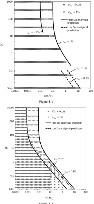
Eq.(21) was found to work very reasonably even near the transition range (Da~ 1), as shown in Figure 4b, where for e_dev 0.1%, predictions at high and low Da overlap. The maximum conversion obtained from this model is

2/3

2/3 2/3

2/3 1 2/3

q

dev dev dev

dev

N B A N

X e e

A Da e A

 _{ } 

 

  _{ }

   

 

, (22)

where N34/3



S1



S3 / 2



_ 5/3(1/ 3)_ is taken from Lévêque‘s solution with Dirichlet boundary condition.

(b) Kinetic control

The applicability boundary under kinetic control is less straightforward. Note that since the developing profile may describe results at high values of zPem, extended Lévêque series (for

short distances) are not applicable. Here, our uniformly valid solution is of interest. The limit of Eq.(9) for low Damköhler number, and small Graetz parameter, is given by

2 2

2

,max ,max ,0 ,max ,0

1 1 1

... 2

C C

R

m m fd m fd

Da z z S z S

X Da

Pe Pe Sh Pe Sh

      _{       }     _ _ _ _ _ _   _{     }   

Since the leading term is the result from our approximate correlation (and Lévêque‘s solution) in the limit of small Da, and the first term in brackets is dominant for z Pem 1:

,max

2 2

1

dev dev

m C C dev

e z

Pe Da Da



    . (24)

The maximum predicted conversion is X_R 2e_dev 2_dev.

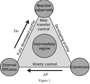
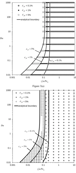
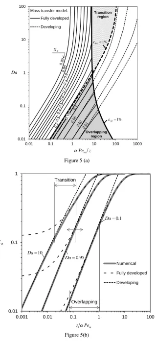
3.4 Validity of mass transfer models

The quality of the conversion prediction by each limiting model is illustrated in Figure 5. The boundaries defined earlier for given values of fd and edev, establish the following picture:

two areas where only one model is able to represent XR with the required accuracy exist near

the Dirichlet limit, separated by a transition region (no satisfactory model). As the Damköhler number decreases, the range of this region decreases, until it is reduced to a single point. For lower values of Da, an overlapping region (both models are suitable) appears and increases as

0

Da . Figure 5 (b) shows these validity ranges for 3 qualitative behaviors (transition in region of finite length, transition in a single point, and overlapping region of finite length) in terms of the observable conversion as a function of the dimensionless distance (limiting models were calculated analytically according to Lopes et al. (2011b)).

This understanding seems to be at odds with previous literature, namely: (i) the overlapping region in Figure 5a has not been recognized before, and (ii) the entrance length (where

1.05 _fd

Sh Sh ) decreases with Da, with a 30-45% reduction for uniform wall concentration relative to the uniform flux asymptote (Shah and London, 1978), in apparent contradiction with e.g. Figure 3. The following additional remarks should be made:

1. The definition of the entrance length in classical literature is mostly based on a (arbitrarily defined) margin for an increase in Sherwood (or Nusselt) number compared to the fully developed value. Lopes et al. (2011a) obtained the same quantities by intersection of the fully developed and developing asymptotes of Sh. This information does not contemplate a transition (or overlapping) region, predicts an increase in the entrance-length as Da decreases, and is directed towards the selection of models for Sherwood number in the analysis of the mass transfer resistances. Here, however, we are interested in analyzing the suitability of conversion

2. Our conclusions are in agreement with other studies in the literature. Lopes et al. (2011b) showed that the error in estimating conversion with one term in Graetz series when Pem z

increases is more significant for high values of Da. Gervais and Jensen (2006) concluded that the importance of the fully developed description increases when Da0, comparing simplified models with the numerical solution. They showed that terms in Graetz series (7), other than the first, decay much faster for lower Da, and this results in a reduction of the absolute error of the fully developed asymptote by one order-of-magnitude at the inlet. This is also observed in the analysis in Supp. Info.

3. Results in sections 3.2 and 3.3 provide the applicability ranges for simplified mass transfer models, explicit on relative errors and for the general case of a wall reaction with any rate. Expressions like these have not been reported, in particular for the case of Robin boundary conditions (finite thermal resistance in the heat transfer problem). Moreover, it is also recognized (Gervais and Jensen, 2006) that the critical value of Graetz‘s number at which Lévêque‘s model is no longer satisfactory cannot be determined from a straightforward approach when Da is finite, and that the required numerical evaluation is tedious.

Since the Graetz problem has been formulated for several geometries (with the calculation of the several coefficients that appear), the results in this section can be applied to shapes other than slit and circular channels. Concerning the use of these results when the flow is also developing, e.g. in the most unfavorable case (Dirichlet boundary condition), we refer to Shah and London (1978) which conclude that the value presented for the thermal entrance length including simultaneously developing flow is a weak function of Pr[or Sc] 0.7 . Hence the validity ranges in the lower practical range of Sc number can be reasonably described by the fully developed laminar asymptote. Another straightforward application of our results is for a flat velocity profile which yields an approximation as Sc0.

4 REGIME MAPPING

Our approach uses the degree of mass transfer control () and the effectiveness factor () as regime definers,

 

surf

surf surf

c c Da

Sh Da c c c

  

  R (25)

 

 

surfcat catcat

c dA c A





R

Consider the isothermal decomposition of a single reactant, with a reaction rate expressed per volume of catalyst by: ˆ

 

ˆ ˆm



1 ˆ ' ˆ



p

V cw k cw c k cw in



 

R . The dimensionless reaction rate (referred

to inlet conditions) is

 

 

 

ˆ _{ˆ (1 ')}

ˆ _{ˆ (1 ' )}

p m

V

p V in

c k c

c

k c c



 

 R

R

R . (27)

Assigning sensible values to  and  (as strict as desired) identifies overall regimes (in the sense that both channel and catalyst present the same level of mass transfer resistance). It was found (Lopes et al., 2012c) that the controlling phenomena changes when a certain value of the diffusion ratio is attained (*). The existence of regimes where mass transfer control is observed more significantly in one phase is also related with this parameter. Thus, regimes of

intra- and inter-phase mass transfer control (where the most important resistance is concentrated exclusively in one phase) are also considered.

The dimensionless quantities presented in section 2 form a multi-parametric space, where the behavior of a given system (combination of design and operation of both microchannel and catalyst) is described by a single point. To reduce the problem so that graphical representation is possible, we consider several ―slices‖ of this parametric space, where we represent the boundary surfaces for the different regimes. Table 2 shows the expressions for these boundaries, which generalize previous work (Lopes et al., 2012c).

The results are shape normalized regarding the channel and catalytic layer cross-sections. Namely, the Sherwood number can be found in the literature for several geometries and suitable boundary conditions with axially and/or peripherally uniform flux or concentration (Shah and London, 1978). The formulation for the effectiveness factor was derived from a generic model (Lopes et al., 2012b), which contains a shape factor that can be fitted to the actual geometry (several examples for catalytic pellets exist (Mariani et al., 2008; Mocciaro et al., 2011)). In its simplest form this is related to the ratio of catalyst volume per surface area and thickness (parameter  given in Eq.(4)). For nonuniform coatings, an improvement to the numerical procedure conceived by Papadias et al. (2000) was given in Lopes et al. (2012b) Since these factors account explicitly for the effect of shape, this methodology is able to compare different geometries in a straightforward manner.

On the contrary, we remark the superiority of the approach presented in Table 2: (i) analytical results, achieving parametric dependence; (ii) generalized treatment for any description of external or internal mass transfer; (iii) ability to capture nonlinear kinetic effects and the relative importance of internal to external resistance; and (iv) accuracy compared to 2D numerical calculations, and respect of the theoretical asymptotes. Hence, the comprehensive picture of the system behavior can be obtained effortlessly.

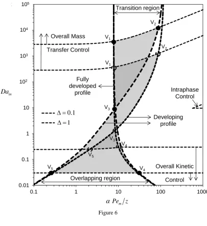
4.1 Intermediate reaction-transport region

The intermediate region can be delimitated with respect to the relative magnitude of the reaction rate (boundaries given in Table 2), as well as to the degree of profile development (results from section 3). This is shown in a Da_inPe_m z plot (Figure 6) for linear kinetics in an annular coating with 1.05 and for two values of the diffusion ratio (fully developed laminar flow).

The dependency of the fully developed and developing boundaries in Figure 6 on the diffusion ratio results from the fact that these were expressed in terms of DaDain in section 3. To

achieve the representation in terms of Dain, the effectiveness factor is calculated by the

analytical solution found in Lopes et al. (2012b). Then, since previous results are written explicitly for Pem z , the nonlinear ( Dain) function is easily evaluated for given values of

in

Da .

The superposition of the reaction-transport and profile development analyzes leads to the identification of an intermediate region (the area in the diagram outside previously defined boundaries). We characterize 5 particular points (vertices) defining this area.

High conversion vertex, V1

If Dain and Pem z are the coordinates of V1 (given by Eqs.(14) and (T5)), then for higher Damköhler number and lower Graetz parameter, the concentration profile can be considered fully developed and mass transfer controlled. An appropriate mass transfer model consists in the first term of Graetz series (7) with eigenvalue and integration constant evaluated at Dirichlet conditions (tabulated values for several geometries exist (Kays and Crawford, 1980; Shah and London, 1978)). Physically, this may correspond to a long microchannel with a fast reaction occurring at the wall, so both reaction and transverse diffusion dominate. This region is associated with high reactant conversion. The minimum conversion, at the vertex in Figure 6, can be calculated from Eq.(15):

2 2 1, 2,

1, 1,

1 (1 ) 0.49

R fd

Hot inlet vertex, V2

The regime delimitated by the boundaries intersecting at V2 is characterized by significant energetic requirements to attain mass transfer control (which increase in developing conditions) and energy dissipation rates associated with high fluid velocities. The reduced residence time in a short channel or at the inlet section penalizes conversion (in the conditions of Figure 6 and according to Eq.(22): X_RN e



_dev A



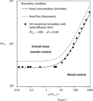
2/30.105, see also Figure 5a). The profile is mass transfer controlled but developing, thus Lévêque‘s solution with constant wall temperature is appropriate. This may represent the state of the inlet section of a channel attaining high conversion at its exit.

When determining the boundary for overall mass transfer control, we have used the value of Sherwood number evaluated with Dirichlet wall conditions (corresponding to low surface concentrations, required to achieve values of  close to 1). However, the correlation for Sherwood number presented in Table 1 has two independent terms, and other forms namely for the developing term may be introduced if desired (e.g. accounting for axial diffusive transport). In order to ascertain the adequacy of the asymptote of Sh_dev with Dirichlet boundary condition, we compare the analytical predictions from Eq.(T5) with the numerical simulation of a 2D model, where the generic Robin condition was implemented at the wall and the axial diffusion term retained. This is shown in a Da_inPe_m z map in Figure 7, where regions of overall mass transfer control (0.90) and mixed control (0.90) can be depicted. The following observations should be made: (a) the regime boundary predicted using the Dirichlet condition is suitable to describe these numerical results; (b) the range of the dimensionless axial distance covered by this picture is wide enough (including the near-inlet region) to describe meaningful conversion in channels with small aspect ratio (0); (c) the variation in the values of  is very weak in this parametric area, and minor differences are observed from the values of Da_in

predicted using the Neumann boundary condition; and (d) adopting a conservative (lower) solution is a design best practice. For all these reasons, we find the Dirichlet boundary condition suitable for our analysis.

Middle point, V3

The intersection of boundaries for fully developed and developing profiles occurs at values of ~ 1

intermediate region appears centered around this point with respect to both profile development (east and west semi-planes) and mass transfer control (north and south semi-planes).

Low conversion vertex, V4

The region in Figure 6 for high Graetz parameter and low Damköhler number delimits an ‗inlet‘ region, in the sense that conversion is low and dominated by convection. High power dissipation is obtained at high flowrates. Conversion at V4 is the maximum observed in this regime and is given by (_fd 0):

2

2 2

2 0

( 3) (1 ) (1 )

~

( ) 2

R

fd fd

S X

K

   

  

 _{  }  _{ }

 

 

 

 

if   * (1), (28a)

2

2 2

0 4

( 3)

~

2( ) 1

R

fd fd

S

X  Sh 

   

  

 

    if   * (0). (28b)

Homogeneous microchannel vertex, V5

High conversions are possible in kinetic control, for sufficiently long microchannels. In this case, transport is dominated by transverse diffusion, thus high dimensionless pressure drops

( 2

~

P L a

 ) are obtained, Eq.(6). The conversion profile can be estimated by the solution for a homogeneous laminar flow reactor. The minimum conversion attainable in this regime is calculated by X_R 2e_dev 0.14 for conditions in Figure 6 and Figure 5a.

Simultaneously developing flow

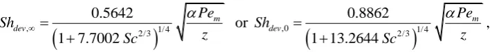
Neumann conditions at the wall), which work in the relevant range of Sc. One can also consider the developing asymptote derived by the same authors and introduce it into the correlation for Sh in Table 1 as





, _2/3 1/ 4

0.5642 1 7.7002

m dev

Pe Sh

z Sc

  

 or ,0



_2/3



1/ 4

0.8862 1 13.2644

m dev

Pe Sh

z Sc

 

 ,

(Dirichlet or Neumann boundary conditions, respectively) while keeping the same value for

, fd

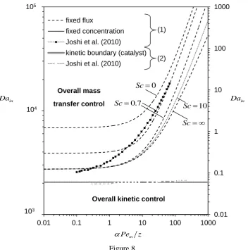
[image:16.595.88.444.115.153.2]

Sh _. Qualitatively, the consequence of this phenomenon is no different from the concentration profile inlet effects considered (enhanced mass transfer towards the coating). In Figure 8, we plot the boundary for overall mass transfer control (according with Eq.(T5), Table 2) for several values of Sc number.

Results from Joshi et al. (2010) are compared with our analytical predictions in Figure 8, after being made dimensionless. It is possible to observe that these system-specific numerical calculations (involving the repetitive solution of partial differential equations for mass transport in channel and catalyst) can be replaced by our simple estimates with all of the previously mentioned advantages. Regarding the mass transfer control boundary, good agreement is observed for Sc~ 0.7 (typical value for air). We also note that under developing conditions, uniform wall flux was assumed by these authors, while uniform wall concentration prevailed downstream. If desired, our correlation for Sh can describe this modeling choice. In our case (small aspect ratio channels), the correlation in Table 1 is appropriate, even near the inlet as shown in Figure 7. Note that the calculation of the kinetically controlled boundary does not require the consideration of the problem at the channel level. Likewise, for overall mass transfer control, the reaction-diffusion problem in the catalyst can be replaced by the diffusional limit of the effectiveness factor, since for the values of  considered, the coating is well within this asymptotic regime. Moreover, the data from Joshi et al. (2010) are only a particular case of the results in Table 2 for  0.1 0.2 , 0.9, 0.9, 1.01, m1, 'k 0 and Sc0.7.

4.2 Kinetic nonlinearities in regime mapping

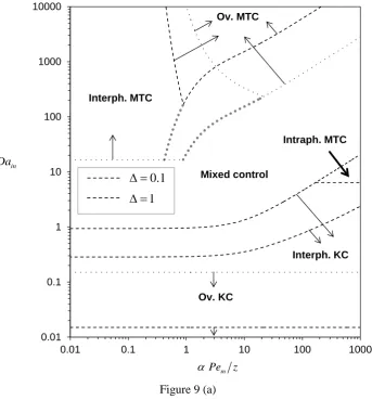
In Figure 9a, we plot the inlet Damköhler number as a function of the Graetz (flow) parameter, for a second-order reaction in a circular channel with laminar flow (coated by a thin annular washcoat, 0.1). The parametric areas of the 4 regimes in Table 2 are identified for two values of the diffusion ratio. In Lopes et al. (2012c), we have presented a temperature diagram, which under certain assumptions (namely concerning the temperature dependence of the reaction kinetics and of physical properties) can also be obtained from the dimensionless representation in Figure 9a. Moreover, here we discuss the influence of other parameters (, m

and k'), and of the reactant concentration distribution at the channel-coating interface on the different boundaries. Therefore, the description becomes more complete, as we also identify the regions of mixed and interphase kinetic control.

The difficulty which prevents the use of the effectiveness factor in an analytical formulation for nonlinear reactions can be debottlenecked by recognizing the relative importance between internal and external mass transfer resistance. This is governed by the value of  compared to

*

 (given in the first column of Table 2). Hence, if the coating is relatively more afflicted by limitation (  *), negligible consumption of reactant in the channel (also near the coating surface) can be assumed in the overall kinetic regime (controlled by the catalyst). The reverse holds if   *. For the mass transfer controlled boundary, the diffusional asymptote of the effectiveness factor and the reactant surface distribution near concentration annulment are useful. This introduces a generic dependence on ‗external quantities‘ (Sh_ and c _, which are easily evaluated in a spreadsheet software) into Eqs.(T5) and (T6) that disappears if m1 (first-order reactions). These are nothing but consequences from kinetic nonlinearities (which further couple the internal and external problem). We also note that regimes are mapped in terms of inlet reference (known) conditions, namely Da_in (since Da may vary axially for the reasons detailed before).

Overall Kinetic control

For these values of the diffusion ratio , the boundary for kinetic control is given by the value of the inlet Damköhler number so that the effectiveness factor is kept above  (e.g. 0.9). This is the limiting factor, which means that external mass transfer proceeds much faster, and thus reactant is distributed uniformly along the interface at a concentration level very close to the inlet one (conversion in the channel is negligible).

Overall Mass transfer control

referred to surface conditions Rˆ_surf and ˆc_surf ) depends on the mass transfer problem in the channel. This yields a distinct area in the diagram, formed by the two boundaries given by Eqs.(T5) and (T6). In particular for low Graetz number, a sharp increase in the required inlet reaction rate is observed. For m1, this happens since the local Damköhler number is decreased by the vanishingly small reaction rate at the fluid-solid interface (severe external mass transfer control). The minimum Damköhler number for overall mass transfer control is obtained at the intersection between both boundaries and is given by













2 1

1 1

~

1 1

m m

in

Sh Sh

Da    

   



   



  (for m1). (29)

If kinetic laws with m1 are suitable to describe such low surface concentrations, then *

   as Pem0, and the regime is defined by the channel with significant internal limitations (i.e. the effectiveness factor is much smaller than in the linear case). There is also a minimum value of Dain resulting from the increase in concentration (steep decrease of

1 1/m

c _ ) and mass transfer coefficient (at a slower rate, included in Sh_) as Pe_m increases. In general, one might say that this occurs around the transition region of  Pe_m z values. In this case, it is noticeable how external mass transfer influences the internal problem, since it is well-known that for the same Thiele modulus, effectiveness increases as m decreases.

Interphase mass transfer control

Apart from the previous overall regime (with low wall concentration, but still allowing for strong gradients to develop in the coating), a purely interphase resistance dominated area is depicted (where the catalyst may be operating in the intermediate or even kinetic regime). For the parameter values in Figure 9, this behavior is not observed with linear kinetics. This regime appears in the same range where overall mass transfer control is defined by the catalyst, according to Eq.(T6). Hence, it occurs when m1, as suggested by the dependence of Eq.(T10) on c _, for low concentrations.

Intraphase mass transfer control

The two boundaries that delimit the intraphase mass transfer controlled regime intersect at a point, whose coordinates (Pem z and Dain) are determined e.g. by Eq.(T9) and:









0

1 1 1

~

m

Sh Pe z

K K

   



     

 

   

Since this regime is found when 0 and 0 (typically K,  and  are O(1)), then it is likely that mass transfer ensues in the entrance regime of the microchannel reactor ( Pe_m z1). Hence, Eq.(30) yields the minimum value of the Graetz number (_~3 ₍ ₎3₎

for which this regime can be found at some value of Dain. The region becomes wider as

m

Pe z

 increases from this value.

Interphase kinetic control and mixed control

When the catalyst coating is comparably more afflicted by diffusional limitations than the channel (i.e.   *), there is a region in the DaPe_m z diagram of interphase kinetic control, where even though transport in the channel is free from limitation, the coating exhibits moderate diffusion effects (i.e.  takes values between the ones used as criteria for the internal regimes). This is found between the overall kinetic and intraphase control regime boundaries. Despite the fact that Sh Sh0 still holds, now  cannot be described correctly by one of its

asymptotes. Nevertheless, the approximation in Lopes et al. (2012b) for thin coatings (see Table 1) is also valid for nonlinear kinetics, by employing a kinetic normalization which is discussed in that reference. For example, for a second-order reaction, it was shown that the approximation has a relative error below 1.6% for coatings with twa. Although the boundary is not explicit

in Dain, it can be written in terms of the Graetz number, which appears in the developing

contribution of Sh0,dev (Table 1). Thus, the boundary can still be obtained analytically

(assigning values of Da_in between the predictions given by Eq.(T1) and (T9)):





0

1 , , ,

in in

Sh Da  Da  m 

 

  . (31)

If 1, Eq.(T3) is recovered. The area delimited by interphase kinetic control and interphase or overall mass transfer control corresponds to moderate limitations in the channel ( between chosen criteria). The influence of the diffusion ratio can be depicted from Figure 9a: the region of interphase kinetic control is much narrower when  increases, while both boundaries of the mixed control area are dislocated towards lower values of Dain.

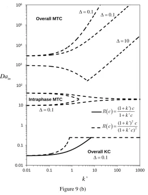
Reactant inhibition effects

Reactant inhibition is translated by the magnitude of the dimensionless constant 'k (k_inh cˆ_in). Figure 9b shows the influence of increasing substrate inhibition on the regime boundaries in a

'

in

Da k plot. The following observations are relevant:

Table 2), increasing the limit value of Da_in up to the value where external mass transfer control is rate-limiting (kinetic independent). For the same parameters, inhibition moves the system from internal to external control.

 An inhibited kinetics requires higher values of Dain to achieve mass transfer control if

internal mass transfer is limiting when 'k 0 (Eq.(T5) is an increasing function of k'). If

 is high enough for relatively slow external mass transfer (compared to the internal one), then the boundary decreases (by one order-of-magnitude in Figure 9b, according to Eq.(T6)), until the minimum value of Dain is dictated by external mass transfer. In mass

transfer limited systems, inhibition increases the local Damköhler number by





2 ( 1)

1k' p m . Thus, the effectiveness factor decreases for the same values of the parameters at the inlet, which explains the previous trends: a lower value of Dain is

required to attain a specified low value of ; and for the same 



Da_in



, higher Dain is

needed to compensate internal limitations.

 The kinetic factor for intraphase mass transfer control (K given by Eq.(T13) with 1

surf

c  ) decreases with 'k . Inhibition restricts the existence and area of this regime. On the other hand, it becomes more prevalent as (mp) increases, which represents the order of reaction in the limit of k' .

 Interphase control would be only observed for  17.3 when 'k 0 (first-order reaction), and this value becomes much higher for larger inhibition constants, since the global order of reaction for the cases in Figure 9b is below 1.

4.3 Catalyst layer design

Because in microchannel reactors the length scale for internal diffusion may be much smaller than the one in the channel, the diffusion ratio  (see Eq.(3)) may take higher values than those found for example, in diffusion through a stagnant film to a pellet in a fixed bed reactor. This is the relevant parameter to compare internal and external resistances (and not the ratios of diffusion timescales D_eff a2 (D t_w2), or of diffusivities Deff D, or of thicknesses a tw, as it is

often found in the literature). Even though mass transfer in the channel and coating are coupled, a Dain  diagram illustrates several features of the coating design (e.g. catalyst loading in

in

Da , porous structure through Deff and layer thickness tw in ). This is plotted in Figure 10

for linear and nonlinear reactions. The following remarks can be made:

expansion is only obtained by increasing the flow parameter, reducing limitations in the channel.

 The opportunity to achieve intraphase mass transfer control decreases as the catalyst diffusion rate increases, but the upper boundary (related to the appearance of non-negligible limitations in the channel) is delayed by moving into the profile developing range.

 This inlet effect also makes overall mass transfer control harder to attain for low/moderate values of the diffusion ratio. For a first-order reaction, low values of the effectiveness factor in the catalyst are reached independently of the channel flow conditions. Thus, the lower limits for intraphase and catalyst controlled overall mass transfer control are given by the same expression (Eqs.(T6) and (T8)), though in different ranges of the diffusion ratio.  For linear kinetics, interphase control is only observed at values of the diffusion ratio larger

than those considered here:  17.3 (value for a fully developed profile from Eq.(T10), 0.9

  ).

 For nonlinear kinetics, the operating map is altered, especially under mass transfer control. This is notorious for a second-order reaction, and in general for any reaction with order above 1. Now both boundaries of the overall regime depend on the Graetz parameter. However, the interphase regime boundary is less sensitive (since for reasonable values of

, it depends on the fully developed value of Sherwood number) and corresponds to the minimum value of the Damköhler number for which strong limitation exists. The existence of this regime is restricted to large diffusion ratios if the profile is developing.

Figure 10a, valid for linear kinetics, also encloses some considerations related with catalyst design, namely loading, volume and existence of limitations to mass transfer. The washcoat loading may be included in the kinetic constant (or pre-exponential factor) as kkˆ (Kočí et al., 2010), where is the concentration of active sites per volume of supported catalyst. The cost associated with the catalyst may be compared among different regimes in the Da_in 

map. Here, we will restrict ourselves to the comparison between operation under overall kinetic (K) and mass transfer (MT) control (the most extreme variation of design and operation). Considering the catalyst cost ( cost ~Vcat , i.e. proportional to the mass of precious metal used)

when operating at these two boundaries for   * ~ 1, the same reaction temperature, effective diffusivity, metal dispersion, channel dimension a and fluid properties:

2

2 ₂

K K

2

MT ,K ,MT MT

cost 3 (1 ) 1

cost

eff

w w

D a L

Sh D t t L

 

 

 

   

 _{  } _

 _{  } ,

microchannel is designed in order to attain the same fully developed conversion in both cases (same feed flowrate), then:





K

MT 1, K K

ln 1 10

~ 3 (1 )

ln (1 )

R

K R

X

L Sh Sh

L Da X w  

          

  . (32a)

Thus, the catalyst cost of a mass transfer limited system is more than 100 times higher, even though the microchannel can be at least 10 times shorter:

2

K MT

MT MT

cost 1 1 1

~

cost Sh 100

         _{ } 

  . (32b)

However, one also needs to take into account the costs due to increased equipment size and pressure drop. The ratio of these costs in kinetic and mass transfer control is assumed to be proportional to L_K L_MT~ 10 _K . Including also this contribution into a ―total cost‖ (cost_total), with the previous order-of-magnitude estimations:

2

total,MT K K K

total,K MT total,K

cost 10 cost

cost 10 10 cost

 

 

 _  _



  . (32c)

This implies that in order for the increased catalyst costs (due to higher loading in mass transfer control) to offset the higher capital and operating costs (due to larger microchannel size to attain the same conversion in kinetic control), the ratio between microchannel (cost_K,ch) and dilute catalyst ( cost ) costs in the kinetic boundary (where e.g. _K 0.9) should be higher than

2 2

K,ch MT

K MT K MT

cost 10 10 10

~

cost 10

  

    . (32d)

The estimated factors can be replaced by exact values, using the expressions above. Nevertheless, assuming a value for D_eff D typical of Knudsen diffusion (e.g. 0.01),

~ 100 μm

a and feasible coating thickness tw1μm, full mass transfer control is economical if

K,ch K

cost

100

cost  .

Although this order-of-magnitude condition may seem unlikely, we note that it is possible that very low loading is required to attain 0.9 in kinetic control (active catalysts; high temperature operation), and that microfabrication and pressure drop costs are significant.

A similar analysis can be conducted when   * ~ 1, i.e. when mass transfer control is defined by the catalyst and kinetic control by the channel, yielding the following considerations regarding the design of the catalyst layer:

2 K

MT

MT MT MT

cost 1

~

cost 100

Sh_{  } 

  (33a)





K

MT ( 1) 0





total,MT K

MT

total,K total,K

cost cost

0.1 100 0.1

cost     cost . (33c)

Operating in overall mass transfer control is beneficial if

K,ch MT

MT K

cost 100 1

~ 100

cost 0.9

 

  . (33d)

The excess of microchannel costs (regarding equipment and pressure drop in kinetic control) required for overall mass transfer control to be beneficial, is minimum when ~ 1, i.e. in the intermediate regime regarding internal/external diffusion. Considering moderate, instead of severe, mass transfer limitations (perhaps in an interphase controlled regime, if attainable) should yield less strict conditions on cost_K,ch cost for the total cost to be reduced, when _K compared to Eqs.(32d) and (33d) (the most unfavorable cases). Thus, it is very likely that

moderateexternal (and when unavoidable, also internal) limitations make the system more cost effective for feasible ratios of the expenditures associated with the channel and the catalyst under kinetic control.

5 DESIGN EVALUATION

5.1 Design in the presence of a constraint on conversion

When a given level of conversion is fixed, Damköhler and Graetz numbers are related (translated by an iso-conversion curve in a DainPem z plot, Figure 11). However, each

point in this curve is characterized by different requirements due to pressure drop and energetic input.

The dimensionless pressure drop P (Eq.(6)) can be written explicitly in terms of the specified value of conversion by making use of simplified results (Lopes et al., 2011b). Figure 5a shows that appreciable reactant conversion will only be found when operation occurs close to full profile development. Consequently, higher dimensionless pressure drops must be faced (i.e. for the same fluid velocity, the microchannel needs to be longer). Under these conditions, the



, _R



P Da X

 dependence for linear kinetics is given explicitly by

 

1

,

1 1

ln

2 1

D

R fd

w Da C Sc

P

X Da Sh_

 

 

 _{  }  _



   . (34)

Calculation of w1 and Sh,fd were detailed in Lopes et al. (2011b). Note that the product

D D

C  f Re is known for several geometries. Eq.(34) is plotted in Figure 11 for specified values of XR, in terms of the inlet Damköhler number (note that Da Dain, but the effectiveness

model with controlling mass transfer and with error fd is calculated as a function of Dain by

Eq.(15). For laminar flow inside a circular channel, if X_R 0.67, the relative error stays below 0.1%.

The asymptote of P close to the regime delimitated by the boundaries intersecting at V1

(high conversion) is



2



,

,

1 2

D fd

fd

C Sc

P P Sh P O Da

Sh Da



  



 

   _   _ 

  for Da . (35)

The minimum dimensionless pressure drop required to attain XR, occurs under total mass

transfer control, and is given by:

1, ,

ln

2 1

D

fd R

w C Sc

P

Sh X

 



 

  _{ }



 . (36)

For the region converging in V5(homogeneous microreactor):

 

1

ln

2 1

D

R

C Sc

P O Da

Da X

 

  _{ }



  for Da0. (37)

The dimensionless pressure drop (channel length) given in (34) is minimized for a given XR,

when Dain (or Da) is increased. On the other hand, the maximum conversion obtained from a

developing profile (associated with lower values of P) is quite low (see Eq.(22)). Thus, to meet a strict target, working on a high- P and/or Da regime is required. Possible improvement keeping the same X , implies moving to the intermediate regime concerning mass R

transfer control, but not with respect to the profile development. The results of Lopes et al. (2011b) are of interest when changes in the intensity of the reaction rate (keeping a fully developed profile) are considered.

5.1.1 Operating limit on Da

The minimum pressure drop P_ guideline is not a clear recommendation since as we showed in section 4, the delimitation of the mass transfer controlled regime may depend on several parameters/criteria. Moreover, other considerations (e.g. external heating demands or catalyst and equipment preservation) only allow this asymptote (Da ) to be fulfilled within a certain non-negligible margin. Thus, it is reasonable to assume that a maximum allowable reaction rate exists (translated into a specified value of Damax, with maximum temperature

and/or catalyst loading). The excess dimensionless pressure drop (Pexc   P P) to be

accommodated by not operating at Da  is taken from (35) and has the following dependence:

, max fd exc

Sh P P

Da   

It is assumed that this maximum value of Da is still close to mass transfer control. Near complete conversion, the additional term to the excess pressure drop expressing the w Da₁

 

dependence is negligible in Eq.(35). If a severe constraint in the value of Da exists (moderate to low values of Da_max), then Eq.(34) should be used to compute P_exc.

The influence of internal diffusional limitations (1) is to increase the dimensionless pressure drop required to attain a conversion XR for the same value of Dain. In this analysis, it

is likely that appreciable diffusional effects in the catalyst appear in overall mass transfer control (intraphase control is more commonly found under developing profile conditions if the diffusion ratio  is not too small; interphase control is only possible for  Sh_ (1) , with  close to 1). In this case, Eq.(38) becomes

, ,max fd exc

in

Sh P P

Da

   

 

 . (39)

Eqs. (38) and (39) are quantitative design rules, which precise the penalties in pressure drop for not meeting the Da  condition exactly. These can be derived by taking into consideration the knowledge of the asymptotic behavior near mass transfer control, given in Eq.(35).

5.1.2 Tolerable P increase

A reduction in Da_in is achieved if a pressure drop above P can be tolerated. If the admissible value of   P P_max P_ is high enough, operation will fall out of mass transfer control (for P_max  P₁  P_) and a conservative estimate for the minimum value of Da is

, 1

min

max 1

fd

Sh P Da

P P P



  

     , (40a)

where 1

,

1 ln

2 1

D

fd R

C Sc P

Sh_ X

 

  _{ }



 . (40b)

For example, if X_R 0.95 in a gas-phase laminar flow, a minimum increase of 19% is required on top of P to fall out of mass transfer control (0.9) in a circular microchannel and this occurs when Da_min16.5. For small increases in pressure drop (remaining under mass transfer control), Eq.(38) can be used with Pexc Pmax and Damax Damin. In this case, it is likely that

diffusional limitations are also present in the catalyst (thus, Eq.(39) applies):

2 2

,min~ ( ) ( max)

in

Da P_ _ P _.

The energetic gain compared to the maximum operating value Damax is

max min 1

max max max 1

1 exc

Da Da P P

Da

Da Da P_ P P_ P

  



  