1
For submission to J. Chem. Phys. 1
2 3 4 5 6
Shape-Independent Model (SHIM) Approach for Studying
7Aggregation by NMR Diffusometry
89
Adrian A. Hernandez Santiago a, Anatoly S. Buchelnikov b, Maria A. Rubinson c, Semen O. 10
Yesylevskyy d, John A. Parkinson e*, Maxim P. Evstigneev b,c* 11
12 13
a
Department of Physics and Mathematics, Faculty of Chemistry, Autonomous University of Puebla, 14
Puebla, Mexico CP 72570 15
b
Department of Biology and Chemistry, Belgorod State University, Belgorod 308015, Russia 16
c
Department of Physics, Sevastopol State University, Universitetskaya str.33, Sevastopol 299053 17
d
Department of Physics of Biological Systems, Institute of Physics of the National Academy of 18
Sciences of Ukraine, Prospect Nauky 46, Kiev-28, 03680, Ukraine 19
e
WestCHEM Department of Pure and Applied Chemistry, University of Strathclyde, 295 Cathedral 20
Street, Glasgow G1 1XL, United Kingdom 21
2 Abstract
23 24
NMR diffusometry has been gaining wide popularity in various areas of applied chemistry for 25
investigating diffusion and complexation processes in solid and aqueous phases. To date, the 26
application of this method to study aggregation phenomena proceeding beyond the dimer stage of 27
assembly has been restricted by the need for a priori knowledge of the aggregates’ shape, commonly 28
difficult to know in practice. We describe here a comprehensive analysis of aggregation parameter-29
dependency on the type and shape selected for modeling assembly processes, and report for the first 30
time a shape-independent model (designated the SHIM-model), which may be used as an alternative in 31
cases when information on aggregates’ shapes are unavailable. The model can be used for determining 32
equilibrium aggregation parameters from diffusion NMR data including equilibrium self-33
association constant and changes in enthalpy, H, and entropy, S. 34
35
Key words: NMR diffusometry, aggregation, self-diffusion, enthalpy, entropy. 36
3 Introduction
38 39
NMR diffusometry has become a popular routine method for characterizing molecular motion 40
via translational diffusion in the solid and liquid states. The approach is extensively used in many areas 41
of chemistry,1-3 the field of research and development of associated methods and data treatments being 42
active and vibrant.4-7 Typical application of NMR diffusometry is to enable molecular aggregation and 43
complexation phenomena to be quantified. So far this has been successfully applied in protein 44
chemistry,8 host-guest chemistry,3 colloid chemistry,9,10 inorganic chemistry,11 supramolecular 45
chemistry12,13 and many other fields of chemical and materials research. A common approach makes 46
use of the Einstein-Smoluchowski relation (eq 1) in order to link the translational diffusion coefficient, 47
D, with the effective hydrodynamic radius (Stokes radius), Reff , and the shape-factor (the so-called 48
Perrin translational friction factor), fP, which characterizes the deviation of the hydrodynamic shape 49
of the studied object from an ideal sphere: 50
6 eff P
kT D
R f
, (1)
51
where k, T, η are the Boltzmann constant, absolute temperature and viscosity, respectively. 52
Equation 1 can only be used if an aggregate’s exact shape is explicitly known, creating a major 53
problem in the use of NMR diffusometry as a general method for studying aggregation phenomena, as 54
discussed in detail here. 55
The magnitude of D is measured through NMR-based diffusion studies and embodies the 56
aggregation parameters of interest. The Perrin translational friction factor, fP, on the other hand 57
contains information concerning the shape of the studied object. Once the link between fP and the 58
geometry of the object is established, eq 1 can be directly applied to fit experimental titration data 59
4
parameters as adjustable quantities. In the basic cases of dimerization or 1:1 complex formation, the 61
diffusion coefficients of the monomer, D1, and dimer (or complex), D2, commonly act as such 62
adjustable quantities.8,10,14 In these instances, knowledge of the exact form of fP is not strictly 63
required. Consequently, the overwhelming majority of known NMR diffusometry applications have 64
successfully used such an approach (for reviews see references 1 and 3). The critical point of departure 65
addressed by us in this article occurs if the aggregation process extends beyond the dimer stage. For 66
such a condition, an explicit model is required describing the dependence of hydrodynamic shape on 67
the dimensions of aggregates formed. Lack of knowledge associated with this dependency creates 68
fundamental difficulty in applying any type of diffusometry for investigating aggregation phenomena. 69
Indeed, the total number of papers dealing with aggregation beyond the dimer assembly stage is 70
notably much smaller compared with simple dimerization or 1:1 complexation. Two main reasons are 71
considered to be responsible for this. 72
Firstly, in practice the shape of aggregates is commonly unknown. Moreover, shape may 73
change as a function of the increasing number of molecules responsible for forming an aggregate. 74
Secondly, only a few classical shapes currently allow analytical equations to be written for the 75
dependence between fP and aggregate geometry (usually in the form of either a sphere, cylinder or 76
oblate/prolate ellipsoid2,13,15). Any other shapes lead to significant difficulties in the computational 77
implementation of the fitting procedure. This is probably the main reason why the majority of 78
published papers introduce the simplest spherical shape to represent aggregates, with a very minor 79
fraction of papers dealing with ellipsoid or other shapes.13,16,17 It is also obvious that a spherical model 80
shape used to represent an aggregate cannot cover the majority of probable shapes encountered in 81
reality. Thus, the dependence of NMR diffusometry on a knowledge of the exact hydrodynamic shape 82
of aggregates remains as the major bottleneck limiting the expansion of this approach towards the 83
5
The aim of the present work is therefore to illustrate the shortcomings of modeling the 85
dependence of the translational diffusion coefficient, D, measured via NMR diffusometry, on defined 86
shape and to find a way to successfully bypass this shape dependency by introducing a modeling 87
approach that is shape-independent (the SHIM approach). In this article NMR diffusometry is used to 88
probe aggregation phenomena in terms of translational diffusion for different types of small molecules 89
known to exert well-characterized aggregation tendencies in solution. To assist the reader, an 90
explanation of the flow and structure of the article is provided as follows. 91
Firstly, a strategy detailing the rationale and criteria behind the choice of molecules for the 92
investigation is laid out. Secondly, for those hydrodynamic shapes most widely encountered already 93
within the literature, expressions are defined that allow equations to be derived for determining the 94
translational diffusion coefficient for each type of shape (Table 1) for illustration and comparison 95
purposes. Expressions for the diffusion coefficients of aggregates of each of these shapes follow from 96
these definitions (viz. Equations 3). The expressions are then used to define the manner by which 97
experimentally measured diffusion coefficients are treated and modeled: weighted averages of values 98
from different sized aggregates are considered based on monomer and dimer diffusion coefficients for 99
each shape separately resulting in Equations 5-8. Modeling of the measured diffusion coefficients for 100
all molecules in the series is carried out with each of the shape-based models in turn to yield a matrix 101
of results illustrative of the current approach adopted throughout the literature and that are treated 102
according to five specific considerations (see Method of selection of the most appropriate model). The 103
analysis of these results and the accompanying considerations are then used to guide the process by 104
which the SHape Independent Model (SHIM) approach expressions are derived by highlighting the 105
link between diffusion and the so-called friction coefficient. This yields expressions 12-14 for the new 106
model, the latter providing a convenient form of the SHIM approach expressed using the 107
6
approach to each of the shape-dependent models are summarized (Table 3) and used for determining 109
the fit between calculated thermodynamic parameters based on the SHIM-model and those reported in 110
the literature for a subset of the molecules used in this study. 111
112
Results and Discussion 113
Strategy of investigation. 114
The target parameter of interest that most fully characterizes the equilibrium aggregation 115
process is the equilibrium self-association constant, K (or Gibbs free energy change on aggregation).27 116
The magnitude of K can be obtained from the dependence of the observable parameter (i.e. 117
magnetization decay in NMR diffusometry data, directly transformed into D) on solute concentration, 118
x0, (i.e. via titration dilution experiments) by fitting these data with a certain model. The NMR-based 119
diffusion aggregation model will always depend a priori on the chosen hydrodynamic shape of the 120
aggregates. For the purposes of this work it was concluded that the shape dependence of the 121
aggregation process be investigated through evaluation of the variation in magnitude of K (derived 122
from the dependence of D on x0) as a function of different models. As a reference K-value, it was 123
proposed that the equilibrium constant derived from 1H NMR titration data be used (i.e. the 124
dependence of proton chemical shifts, δ, on x0) recorded in parallel with NMR-based diffusion data on 125
the same solutions. Such a strategy allows the well-known dependence of K on concentration range to 126
be ruled out of influencing the investigation together with the type of experiment used to produce the 127
titration curves (see ref. 28 for a full review). 128
7 130
Fig. 1 Test molecules used for studying aggregation phenomena by means of NMR diffusometry. 131
132
Selection of the compounds for study (see Materials and Methods and Figure 1) was dictated 133
by the following set of criteria: 134
a) the molecules must feature different shapes in order to create differently shaped aggregates. 135
8
molecule alone and in each particular case must be discussed separately. In particular, the 137
aromatic molecules not containing heavily branched side chains, viz. compounds 2, 3, 4 and 7 138
should follow a linear-type aggregation process, presumably matching cylindrical or ellipsoid 139
shapes of aggregates, whereas for the rest of the molecules it is difficult to predict the 140
aggregate’s shape, 141
b) the aggregation tendency of the test compounds must vary in order to account for the 142
dependence of the measured value of D on the magnitude of the self-association constant. The 143
set of molecules selected feature a dispersion of K values spread over several orders of 144
magnitude ranging from 11 M-1 (for 3) up to 5600 M-1 (for 7), 145
c) the test molecules must contain enough well-resolved non-exchangeable protons to allow 146
reliable D(x0) and δ(x0) curves to be established. 147
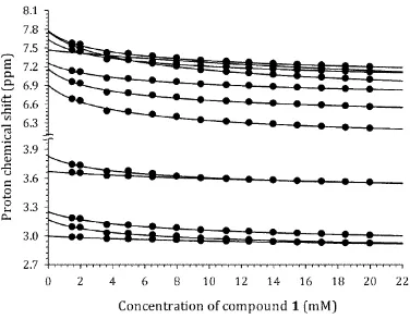
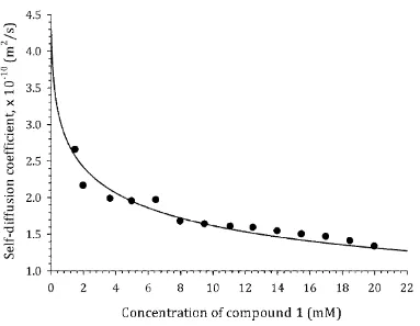
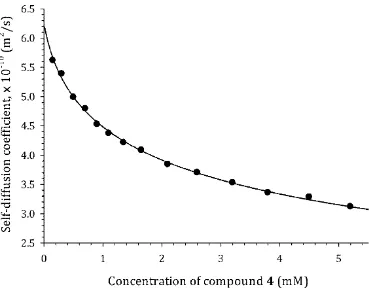
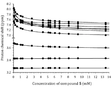
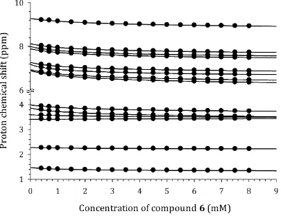
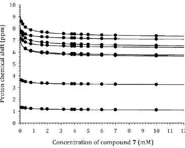
Experimental self-diffusion, Dobs(x0), and chemical shift, δ(x0), data are shown in Fig. 2 for 148
compound 4 as a typical example. The data for the remaining compounds are provided within the 149
Supporting Information. The behavior of the experimental curves is qualitatively similar for all of the 150
molecules studied, viz. shift of the δ(x0) curves to lower NMR frequency and shift of Dobs(x0) curves to 151
lower values of diffusion coefficients on increasing the solute concentration. These features are typical 152
of aggregation processes occurring by stacking of aromatic chromophores.10,13,27 It is also worth noting 153
that the concentrations of the test molecules used to obtain the titration curves fall into the low 154
millimolar range, which is negligible compared with the concentration of the solvent molecules (D2O). 155
This allows any changes in viscosity of the solvent to be considered negligible and therefore capable of 156
9 158
Fig. 2 Experimental dependence of self-diffusion coefficient, Dobs(x0), and proton chemical shift, δ(x0), 159
on concentration, x0, for 4, PF, taken as a typical example. 160
161
Hydrodynamic shapes. 162
As discussed in the preceding dialogue, there are three main types of shapes currently in use in 163
the majority of NMR diffusion studies concerning aggregation phenomena, namely the sphere, the 164
cylinder and the ellipsoid. Each of these general models can be further reduced to more specific shapes. 165
The link between the types of shape and the translational diffusion coefficient are detailed below. 166
Equation 1 can be re-written as: 167
kT D
r
, (2)
168
where rrspherefP is the friction coefficient in which rsphere 6 Reff is the coefficient of translational 169
resistance for the sphere. It should be noted that in the case of the ellipsoidal or cylindrical geometries 170
eff
R denotes the radius of the sphere of equivalent volume.29 By evaluating the Perrin translational 171
friction factor, fP, for a given shape, the final equation for diffusion coefficient can be obtained 172
10
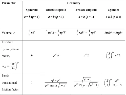
Let pa b be the axial ratio where a and b are the major and minor semi-axes of an ellipsoid 174
(or the half-length and radius of a cylinder). Note, if a = b then one gets the degenerate case of a 175
sphere. Once these notations are introduced, the Perrin translational friction factors can be written in 176
exact form.29,30 Table 1 summarizes all the formulas for the above-mentioned geometries. Evaluating 177
eff
R and substituting it into the equation for the friction coefficient, r, along with Perrin factor, fP, 178
yields the final equations for translational diffusion coefficients in explicit form (last row in Table 1). 179
[image:10.612.65.563.339.718.2]180
Table 1 Collection of formulas necessary to derive equations for translational diffusion coefficients for 181
the most widely used geometrical shapes 182
183
Parameter Geometry
Spheroid a = b (p = 1)
Oblate ellipsoid a < b (p < 1)
Prolate ellipsoid a > b (p > 1)
Cylinder a ≠ b (p ≠ 1)
Volume, V 4 3
3b
2 2 3
4 4
3a b 3 p b
2 3
4 4
3ab 3 pb
2 3
2ab 2 pb
Effective hydrodynamic radius, 1 3 3 4 eff V R
b p b2 3 p b1 3
1 3 1 3
3
2 p b
Perrin translational friction factor, 1 2
1 3 2
1 arcsin 1 p p p
21 3 2
1
ln 1
p
p p p
1 3 2 3
11 P f Translational friction coefficient,
6 eff P
r R f
6b
1 3 2
2 1 6 arcsin 1 p p b p
2 2 1 6 ln 1 p b p p 6 ln
p b p Translational diffusion coefficient,
DkT r
6 kT
b
2
1 3 2
arcsin 1
6 1
p kT
b p p
2 2 ln 1 6 1 p p kT b p ln 6 kT p b p Note: In the case of an aggregate of cylindrical shape 0.312 0.565 p0.100 p2 (a discussion of 184
the parameter ν is detailed in the dialogue which follows later in this work). 185
186 187
Hydrodynamic models of aggregation. 188
The most common case of molecular aggregation is the growth of aggregates by sequential 189
addition of monomers.27,31 Hence, the geometrical parameters of any immediate aggregate (a and b) 190
and, consequently, the diffusion coefficient, D, in eq 3, can be expressed via the number of molecules, 191
i, in the aggregate. 192
For an oblate ellipsoid, p1 so that the major semi-axis, a, corresponds to the radius of the 193
molecule (d/2, where d is the diameter), whereas the minor semi-axis, b, corresponds to half the sum of 194
monomers constituting an aggregate: ad 2, bLi 2, pd Li
, where L is the average thickness 195of a monomer unit. As an indicator, for molecules containing aromatic rings, it is common practice to 196
12
surfaces.15 In a prolate ellipsoid, p1 so that the major semi-axis, a, corresponds to half the sum of 198
monomers constituting an aggregate, whereas the minor semi-axis, b, represents the radius of the 199
molecule, similar to that in the cylindrical models: a Li 2, bd 2, pLi d. Considering an 200
aggregate as a spheroid, the former is represented as a sphere of equivalent volume, which is the sum 201
of equivalent volumes of constituent monomers. Thus, the equivalent radius, b, can be evaluated in 202
terms of the monomer diameter, d: bi1 3d 2. Substitution of these relations into the equations from 203
the last row of Table 1 yields the diffusion coefficients of aggregates,Di, for the standard set of 204 shapes: 205
1 3 22 3 2
1 3 2 2 2 Sphere: 3 arcsin 1 Oblate ellipsoid: 3 1 ln 1 Prolate ellipsoid: 3 Cylinder: ln 3 i i i i kT D di d Li kT D
Li d d Li
Li d Li d
kT D
Li d
kT
D Li d i
Li (3) 206
Specifically for the cylindrical model a correction for the end effects is sometimes introduced in the 207
form of a correction factor v i
0.3120.565d
Li 0.100
d
Li
2.13,32 208Equations 3 provide explicit interrelation between Di and i for basic shapes. It is, however, 209
apparent that the shapes of aggregates at the monomer and dimer level may significantly deviate from 210
those assumed for larger aggregates. Considering that the fraction of monomers and dimers typically 211
dominate over other species in solution (if the aggregation process is not strongly cooperative), it is 212
reasonable to introduce the diffusion coefficient of monomer, D1, and dimer, D2, as adjustable 213
13
and/or dimer. Now, eq 3 may be used to express the experimentally observed translational diffusion 215
coefficient obtained via NMR diffusion experiments, Dobs, as a weighted average of Di:9,33 216
0
1
obs i i
i
D D x
x
, (4)217
where xi ix Kx1
1
i1 is the concentration of an aggregate containing i molecules. 218Each model was used in two forms, viz. with variation of D1, and with variation of D1/D2. 219
Below are listed the set of final expressions used in the analysis of experimental NMR diffusometry 220
data with the quantities in square brackets describing the adjustable parameters in the model. 221
222
SPHERICAL: 223
[D1, D2, K, d]
1 2 3
1
obs 1 1 2 1
3 0 2 3 i i x kT
D D Kx D i Kx
x d
, (5)224
OBLATE ELLIPSOID: 225
[D1, K, d]
2 2 1 1 3 1obs 1 1 2 2
1 0
arcsin 1 1
1 arcsin 1
i
i
d Li d L
x
D D i Kx
x d L d Li
, (6.1)226
[D1, D2, K, d]
2 1 1 3 1obs 1 1 2 2 3 1 3 1 2
3 0 arcsin 1 2 3 1 i i d Li x kT
D D Kx D i Kx
x L d d Li
, (6.2)227
PROLATE ELLIPSOID: 228
[D1, K, d]
2 2 2 1 1obs 1 1 2 2 2
1 0 ln 1 ln 1 i i
Li d Li d
x L d
D D i Kx
x L d L d Li d
. (7.1)229
[D1, D2, K, d]
2 1 1obs 1 1 2 1
2 2 3 0 ln 1 2 3 i i
Li d Li d
x kT
D D Kx D i Kx
x Li d
. (7.2)14 CYLINDRICAL:
231
[D1, K, d]
1 1
obs 1 1
1 0 ln ln 1 i i
Li d i
x
D D Kx
x L d
, (8.1)232
[D1, D2, K, d]
1 1
obs 1 1 2 1
3 0 2 ln 3 i i x kT
D D Kx D Kx Li d v i
x L
. (8.2)233
234
The monomer concentration, x1, for all the models listed above takes the standard form for isodesmic 235 aggregation:9,15,17,27 236 0 0 1 2 0
1 2 1 4
2
Kx Kx
x
K x
. (9)
237
The self-diffusion data, Dobs(x0), were also treated using the dimer model of aggregation, which 238
assumes that no aggregation proceeds beyond the dimer stage:27 239
240
DIMER: 241
[D1, D2, K]
1 2
obs 2
0 2
1 1 8
D D
D D
Kx
. (10)
242
The proton chemical shift titration data, δ(x0), used as a reference, were treated according to the 243
standard isodesmic model of self-association:27 244
245 1
H NMR ISODESMIC MODEL 246
[δ1, δ2, K]
0 1
2 1
0 00
2Kx 1 4Kx 1 x
Kx
, (11)
247
where δ1, δ2 are chemical shifts in monomer and dimer states, respectively. 248
15 Method of selection of the most appropriate model. 251
The following considerations have been taken into account when analyzing the results of 252
computations over different models and different molecules: 253
1. All of the adjustable parameters must take physically meaningful positive values. Otherwise the 254
model is considered inappropriate. 255
2. It is assumed that for a well-performing model, the magnitude of K should be as close as possible 256
to the 1H NMR derived constant obtained under similar solution conditions. However, it is known 257
that different methods may yield different values of K and none of them may be considered as the 258
most exact. This is also the case when comparing NMR diffusion and 1H NMR-derived constants. 259
It is accepted that if NMR diffusion and 1H NMR-derived constants differ by an order of 260
magnitude, the model is considered inappropriate. 261
3. The discrepancy function, Δ (or, alternatively, the goodness of fit, R2), i.e. the mean square 262
deviation of the theoretically calculated D values from the experimentally observed Dobs values, 263
served as an additional criterion for selecting the best performing model, viz. the lower the value of 264
Δ (or the higher the value of R2), the better the model. One important point should be taken into 265
account. Different models tested in the present work use different numbers of search parameters 266
(between 2 and 4). Consequently the discrepancy of the model with a lower number of parameters 267
may be slightly worse than that of the other models having larger numbers of parameters. This fact 268
does not necessarily imply a poor model. However, if the discrepancy of a certain model in the 269
analysis appears to be an order of magnitude worse than that of the others, it can serve as an 270
indication that this model is not appropriate. 271
4. The magnitude of D1 must always be higher than D2. Taking the spherical model as an initial 272
approximation, it follows that D D1 2 3 2 1.26.29 This relationship was taken as a guess value 273
16
the self-diffusion process for the monomer and dimer for the selected set of molecules was 275
performed (Table 2). It may be seen that on average the relationD D1 2 is rather close to the 276
spherical approximation. The model which gives values outside the range 1D D1 2 2 must be 277
treated with caution. 278
5. The physically meaningful values of the d parameter in the models (5)-(8) are strongly dependent 279
on the geometry of the molecule, but may be limited from the upper and lower side by taking into 280
account the typical dimensions of aromatic heterocycles. For the set of the compounds studied in 281
the present work it was assumed that the values of d falling outside the range 0.3 nm < d < 3 nm are 282
erroneous. 283
284
Table 2 Magnitudes of monomer (D1) and dimer (D2) translational diffusion coefficients (10-10 m2/s) in 285
D2O calculated by means of molecular dynamics simulation 286
Molecule D1 D2 D D1 2†
2 6.7 5.5 1.22
3 11.3 8.8 1.28
4 10.4 8.2 1.27
† Note: similar but higher values of D1 and D2 have been obtained in H2O (data not shown), preserving 287
virtually the same values of D D1 2 as those shown in the table. 288
289
Analysis of the results of calculations using various hydrodynamic models. 290
The result of computations covering the set of hydrodynamic models described above and 291
applied in order to fit the Dobs(x0) titration (dilution) data, and the reference calculations of the self-292
17
presented in Table 3 (Strategy 1) as qualitative representations and in the Supporting Information in a 294
quantitative form. The following conclusions may be drawn from inspection of these results (only for 295
Strategy 1 for now), omitting in the first instance the results obtained from the dimer model: 296
(i) The results for the molecules containing (2, 3, 4, 7, 8) and not containing (1, 5, 6) a rigid 297
aromatic chromophore do not show clear preference for a particular model suggesting that the 298
aggregation is relatively insensitive to the type of hydrodynamic model used. The latter may be 299
interpreted by the fact that the aggregation of these compounds in the concentration range studied 300
(limited by the solubility) is not pronounced, i.e. the contribution from aggregates of higher order 301
than dimer is relatively unimportant, thus attenuating the influence of the selection of the type of 302
shape in the model. The quality of fit of the diffusion data with various models for these 303
compounds is very similar and does not allow unambiguous selection of the best model by this 304
criterion; 305
(ii) The ellipsoid and cylindrical models with three adjustable parameters (i.e. eqs 6.1, 7.1, 8.1) for 306
the majority of molecules failed to describe the experimental data, whereas addition of D2 as a 307
fourth adjustable parameter (i.e. eqs 6.2, 7.2, 8.2) enabled the data to be fitted with meaningful 308
outcomes. Hence, it is recommended that D2 be always used in an explicit form when carrying 309
out numerical analysis of self-diffusion data for aggregation; 310
(iii) An apparent improvement of the performance of the cylindrical model is seen when the 311
correction for the end effects is introduced, which is in agreement with the current view; 13,32 312
(iv) The spherical model with four parameters (eqs 5) showed the best performance as compared with 313
other models. It allows partial explanation as to why the spherical model has so far been applied 314
in the majority of cases for investigation of aggregation processes, as alluded to in the 315
18
(v) Even though the shape-dependent models have, in general, shown good performance for different 317
shapes of molecules, there remains a problem in verifying the reliability of the calculated 318
magnitude of the parameter d, which is not possible to estimate based on the shape of the 319
molecule or its dimer. Moreover, the results of calculations presented in the Supporting 320
Information demonstrate high dispersion of d across the models studied. This result is difficult to 321
interpret and is most likely unreliable. Hence, any use of spherical, ellipsoid or cylinder model 322
must be treated with caution. 323
In summary, it is possible to establish initially that the aggregation processes of the test 324
compounds appears not to be strongly related to the type of shape used in the hydrodynamic model. 325
The additional test of this assumption was accomplished by varying D1 and D2 simultaneously such 326
that the condition D D1 2 32 1.26 was always matched during the data fitting procedure, which is 327
compliant with the results of molecular modeling (see above), and allows the number of adjustable 328
parameters to be reduced. The results of these computations are shown (Table 3, Strategy 2). 329
According to this approach, the spherical and cylindrical models (13 and 16) appear to be most 330
appropriate for the largest number of molecules studied, suggesting that Strategy 2 (three adjustable 331
parameters) may be recommended for the numerical analysis of self-diffusion data for self-aggregating 332
systems using these models. However, the dispersion of d remains the most problematic issue. 333
In summary it may be concluded that the use of shape-dependent models (either spherical or 334
cylindrical) with Strategies 1 or 2 is applicable only if some a priori information regarding an 335
aggregate’s shape is available enabling the value of d to be estimated. If such information is absent 336
(which is the most likely scenario in practice), the present work shows that based on goodness of fit 337
data alone, it is not possible to unambiguously select the most appropriate shape-dependent 338
hydrodynamic model. 339
19 341
342
Development of shape-independent model (SHIM-model). 343
Taking into account i) the relative insensitivity of the aggregation parameters derived from 344
diffusion NMR data to the shape selected in the model, ii) the difficulty in practice of predicting the 345
shape of aggregates based only on the structure of monomer or dimer, and iii) the difficulty in a priori 346
knowledge of the magnitude of the d parameter, the possibility of developing a model which does not 347
introduce any assumptions about the type of shape and is free of the problem of the d parameter, is 348
considered here as an alternative approach. 349
The key quantity in eq 2 is the friction coefficient, r, which appears in the standard equation for 350
a resistance force in solution experienced by a molecule on moving with speed, v, viz. F r v. 351
Force is an additive quantity. Hence, to a first approximation, this additive property can be transferred 352
to r as well. Based on this assumption, it is possible to express the stepwise addition of a molecule to 353
an aggregate in terms of a stepwise addition of the same quantity, Δr, to r, i.e. ri r1 r i
1 , where 354i is the number of molecules in an aggregate. Diffusion and friction coefficients are linked to each 355
other via eq 2, i.e. 356
i i
r kT
D ; at i 2, 2 2 kT D r . 357
The latter allows the expression
1
2 D
kT D kT
r
to be derived. Further use of this relation to derive the 358
expression for the NMR observable self-diffusion coefficient follows as: 359
1
1 2 1
1 1
1 0 0 2 2 1 1 2
i i
obs i
i i
iD D Kx
x x
D iD D
x x D i D D
, (12)360
20
Equation 12 can finally be expressed in a more convenient form, representing the shape-362
independent model (the SHIM-model): 363
364
SHIM-model: 365
366
[D1, D2, K] obs 1 1
1 00
1 i
i
x i
D D Kx
x i
, where 21 2
D
D D
. (13)
367
368
Equation 13 can be further rewritten in more convenient form using the hypergeometric function, F, as 369
follows: 370
371
1 2 1
obs 1 1
0 1 2 1 2
2, ; ;
x D D
D D F Kx
x D D D D
. (14)
372
373
Such notation avoids the need for direct programming of the infinite summation in eq 13 being 374
replaced instead with the standard hypergeometric function, available in the majority of mathematical 375
software packages (e.g. MATLAB or MathCAD). 376
The results from computations using the SHIM-model are shown in Table 3 for Strategies 1 377
and 2, and in the Supporting Information. Within Strategy 1, the SHIM-model with three adjustable 378
parameters gives the same performance as the spherical model with four parameters (which is 379
considered as the best over others) with nearly the same goodness of fit (see Supporting Information). 380
Within Strategy 2 the SHIM-model has succeeded for all test molecules alike versus the spherical 381
model. Recall that the SHIM-model is free of the problem of the d parameter discussed above, and 382
gives nearly the same goodness of fit as the spherical model in both strategies but with lower number 383
21
the hydrodynamic shape of aggregates is unknown and the d parameter cannot be predicted, the SHIM-385
model has an advantage over any other shape-dependent model. 386
22
Table 3 Qualitative indication of when the model succeeded (shaded cell) or failed (blank cell) to fit 388
experimental data and/or to match the reference parameters 389
390
Models Molecules
No. of model in Supporting Information
type of the shape
number of adjustable parameters
1 2 3 4 5 6 7 8
Strategy 1 (D1 and D2 are independent variables)
1 Dimer model 3
2 Spheroid 4
3
Oblate ellipsoid 3
4 4
5
Prolate ellipsoid 3
6 4
7 Cylinder without correction
3
8 4
9 Cylinder with
correction
3
10 4
11 SHIM-model 3
Strategy 2 (fixed ratio D1/D2 = 1.26)
12 Dimer model 2
13 Spheroid 3
14 Oblate ellipsoid 3
15 Prolate ellipsoid 3
16 Cylinder 3
17 SHIM-model 2
23
In order to provide additional reliability tests for the computational results obtained using the 393
SHIM-model (specifically model 11 in Table 3) with respect to the number of experimental points 394
measured, we recalculated the set of adjustable parameters by sequentially excluding one to three 395
experimental data points randomly selected from the entire range of measured concentrations for each 396
compound studied. The results are presented in the Supporting Information and clearly suggest that 397
exclusion of even three data points does not change the magnitude of the adjustable parameters to any 398
significant extent that could be considered to alter the conclusions formulated above regarding the 399
comparison of different models. 400
401
Peculiarity of the dimer model with respect to self-diffusion data. 402
The use of the dimer model to treat self-diffusion data (intentionally omitted above) is linked to 403
the fundamental problem associated with dimer and isodesmic models. These are indistinguishable 404
from one another with respect to the goodness of fit of the titration data (see ref. 28 for a review). This 405
must therefore be discussed separately. More simply put, it is not possible to distinguish between dimer 406
and indefinite aggregation based on the magnitude of the discrepancy function, Δ, only. It has been 407
shown28 that this indistinguishability originates from the use of two basic assumptions in the model: (i) 408
the observable is given as an additive quantity over the molecules forming an aggregate; (ii) the 409
observable is influenced only by nearest neighbors in an aggregate. The majority of known 410
experimental methods implicitly or explicitly use these assumptions in treating the aggregation process. 411
Hence, the property of indistinguishability is intrinsic to many widespread physico-chemical methods 412
such as NMR, spectrophotometry, microcalorimetry and so forth. It was also suggested28 that any 413
approach not meeting any of these two assumptions may potentially resolve the problem of 414
indistinguishability. It is therefore worth considering whether this is possible within the diffusion NMR 415
24
The translational diffusion coefficient, D, is an additive quantity with respect to aggregates 417
present in the system under the fast exchange regime on the NMR timescale. However, it is not an 418
additive quantity with respect to the molecules forming an aggregate and has no relationship to nearest 419
neighbor assumptions. Hence, in theory diffusion NMR data when treated according to either dimer or 420
indefinite models should result in different goodness of fit values depending on whether the system 421
aggregates beyond the dimer stage or not. Table 3 shows that the dimer model has reliably succeeded 422
for 3, 8 and for the remaining systems the dimer model appears to be inappropriate. In fact this result 423
highlights which category of aggregation state (dimer or extended aggregate) best matches each of the 424
molecules studied. Although investigation of the dimer-to-indefinite aggregation by NMR 425
diffusometry is a matter of special investigation, the preliminary results obtained in the present work 426
suggest the potential ability of the technique to distinguish between the dimer and indefinite modes of 427
aggregation and resolve the problem of indistinguishability. 428
429
Application of the SHIM-model to thermodynamic analysis of aggregation. 430
A common approach to determine changes in enthalpy, ΔH, and entropy, ΔS, of aggregation is 431
to measure the temperature dependence of an experimental observable and then to fit it to an 432
aggregation model (often the same one used to fit the titration data), in which the self-association 433
constant is substituted with the van’t Hoff relation34,36 434
RT
H
R
S
K
exp
, (15)435
where R is the gas constant. 436
A similar approach can be used to obtain ΔH, ΔS from the dependence of Dobs on temperature 437
by substituting eq 15 into eqs 5-11, 14 for either the shape-dependent models or the SHIM-model. 438
However, for the self-diffusion data, the dependence of D1 and D2 on T must also be taken into 439
25
Let us designate D1 and D2 as D1,2. Hence, eq 2 takes the form 441
1,2 kT D r T , (16)
442
where r(T) is the temperature-dependent coefficient of friction. 443
The dependence of r on T is due to the dependence of viscosity, η, on T, allowing eq 16 to be 444
rewritten in the form: 445
1,2 1,2 T D C T , (17)
446
where C1,2 is a temperature-independent constant. 447
The viscosity of D2O depends on T as13,37 448 164.97 lg 4.2911 174.24 T (18) 449
and at T=298 η298=0.0011 kg·m-1·s-1. 450
As long as the exact magnitudes of D1 and D2 are available from the analysis of titration data at 451
fixed temperature (in the present work at T = 298 K, or 333 K for 6), see above), i.e. D1,2298 is known, 452
so the expression for D1,2 at any temperature can be written as 453
298 298 6 298
1,2 1,2 3.691 10 1,2
298
T T
D D D
T T
. (19)
454
It follows that the algorithm for obtaining thermodynamic parameters from self-diffusion data should 455
occur by fitting the Dobs(T) curve with the selected model (eqs 5-11, 14) in which the parameters K, D1 456
and D2 are replaced with eq 15 and eq 19. There are only two parameters in such an approach, viz. ΔH 457
and ΔS, although in practice additional small variation of D1,2298 may also be introduced. 458
Equation 19 may be independently tested for appropriateness against the 459
tetramethylammonium, used as a reference in all NMR experiments in the present work. If eq 19 is 460
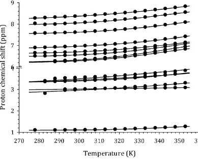
26
NMR), the temperature-dependent diffusion, Dobs(T), for the TMA signal must be fitted with eq 19 462
with good quality having just one adjustable parameter, D1,2298. Figure 3 shows the experimental 463
Dobs(T) curves for TMA in the self-aggregation studies for the two selected compounds 2 and 4. The 464
goodness of fit in all cases was not worse than R2=0.99 indicating that eq 19 is appropriate in 465
thermodynamic analyses using self-diffusion data. 466
467
Fig. 3 Experimental Dobs(T) curves for TMA in the self-aggregation studies and their fitting curves for 468
2, EB (□ fitted with solid line) and 4, PF (× fitted with dashed line) 469
470
Thermodynamic analysis of aggregation based on self-diffusion data has been performed in the 471
present work taking as examples different structured compounds 1, 2, 3, and 4 which have been 472
thoroughly characterized previously in terms of the enthalpy and entropy of aggregation (for reviews 473
see refs. 17, 34, 38). Experimental measurements as well as the numerical analysis were performed 474
against two datasets namely δ(T) and Dobs(T) measured in parallel for similar solutions. The 475
computation of ΔH, ΔS from δ(T) was accomplished by using eq 11, and from Dobs(T) by using eq 13 476
of the SHIM-model. The results are shown in Table 4. Good correspondence can be seen between the 477
diffusion, 1H chemical shift and literature data suggesting that NMR diffusometry with the SHIM-478
27 480
Table 4 Changes in enthalpy (kJ·mol-1) and entropy (J·mol-1·K-1) upon aggregation 481
Data
1 2 3 4
ΔH° ΔS° ΔH° ΔS° ΔH° ΔS° ΔH° ΔS°
1H, δ(T) –31 –0.08 –26 –40 –25 –63 –38 –73
Diffusion, Dobs(T) –40 –0.04 –29 –50 –21 –46 –41 –74
Literature17,34,38 –40 –0.06 –23 –31 –21 –50 –46 –101
482 483
Experimental Section 484
485
Chemicals 486
1 (4-(2'-(4-hydroxyphenyl)-1H,3'H-[2,5'-bibenzo[d]imidazol]-6-yl)-1-methylpiperazin-1-ium 487
chloride, Hoechst 33258, purchased from Sigma-Aldrich), 2 (3,8-diamino-5-ethyl-6-488
phenylphenanthridin-5-ium bromide, ethidium bromide (EB) purchased from Sigma-Aldrich), 3 (1,3,7-489
trimethyl-1H-purine-2,6(3H,7H)-dione, caffeine (CAF) purchased from Sigma-Aldrich), 4 (acridine-490
3,6-diamine, proflavine (PF), purchased from Sigma-Aldrich), 5 (sodium 7-amino-4-hydroxy-3-((E)-491
(2-sulfonato-4-((E)-(4-sulfonatophenyl) diazenyl)phenyl)diazenyl)naphthalene-2-sulfonate, supplied as 492
a gift), 6 (N-[5-({[5-({[4-({[3-(dimethylamino)propyl]amino}carbonyl)-5-isopropyl-1,3-thiazol-2-493
yl]amino}carbonyl)-1-methyl-1H-pyrrol-3-yl]amino}carbonyl)-1-methyl-1H-pyrrol-3-yl]-2-494
quinoxalinecarboxamide trifluoroacetate – AIK-18/52, supplied as a gift), 7 (N-(5-amino-9H-495
benzo[a]phenoxazin-9-ylidene)-N-ethylethanaminium chloride, Nile Blue (NB) – C. I. Basic Blue 12 496
purchased from Sigma-Aldrich) and 8 (sodium 1-amino-9,10-dioxo-4-((3-((2-((2-497
28
gift) (Figure 1) were acquired and used without further purification. D2O was supplied by Sigma-499
Aldrich. Samples were prepared by making suitably concentrated stock solutions in D2O and these then 500
used as the basis to create serially diluted samples for study by NMR spectroscopy. Measurements 501
were made by diluting samples within their NMR tubes to avoid issues encountered from experience 502
when samples are divided or when separate samples are used to generate a series of concentration-503
dependent NMR data. Sample concentrations in each case are shown in the Supplementary 504
Information. 505
506
NMR measurements. 507
NMR spectra were acquired at a magnetic field strength of 14.1 Tesla using a Bruker Avance 508
II+ NMR spectrometer operating at a 1H resonance frequency of 600.13 MHz and working under 509
TopSpin version 2.1 (Bruker Biospin, Karlsruhe, Germany) on an HP XW3300 workstation running 510
Windows XP. Typically all NMR spectra were acquired on the prepared samples using a broadband 511
observe probe-head equipped with a z-pulsed field gradient coil [BBO-z-atm]. 512
1D 1H NMR spectra were acquired over a frequency width of 12.3 kHz (20.55 ppm) centered at 513
a frequency offset equivalent to 6.175 ppm into 65536 data points during an acquisition time aq = 2.66 514
s with a relaxation delay d1 = 2 s for each of 32 transients. The assignment of proton signals was 515
accomplished with the aid of 2D heteronuclear [1H, 13C] HSQC and HMBC NMR data and 2D 516
homonuclear [1H, 1H] COSY, TOCSY and NOESY NMR data. All measurements have been 517
performed under the fast exchange regime on the NMR chemical shift timescale at T = 298 K with the 518
exception of specific variable temperature measurements, which were performed over a range of 519
temperatures from 278 K to 343 K. Chemical shifts were measured relative to an internal reference of 520
tetramethylammonium bromide (TMA) and recalculated with respect to (sodium 2,2 dimethyl 2-521
29
Diffusion measurements were carried out as previously described18 using a bipolar gradient 523
pulse program (Bruker pulse program ledbpgppr2s) in which presaturation was used to suppress 524
residual solvent signal during the recycle delay. Typically 32 gradient increments were used by which 525
the gradient strength was varied linearly in the range 2% to 95% of full gradient strength (54 G/cm 526
with a rectangular gradient) using a sine-shaped gradient profile. Typically the gradient pulse duration 527
was set to 1 ms and the diffusion period to 200 ms. With increasingly dilute samples, the number of 528
transients was increased accordingly in order to allow for diffusion coefficients to be evaluated with a 529
reasonable fit of the experimental data to theory (i.e. number of transients (ns) per FID varied in the 530
range 32 ns 256 for sample concentrations in the maximal range from 31 mM to 100 M). 531
Diffusion data were processed under TopSpin (version 2.1, Bruker Biospin) using the T1/T2 analysis 532
module in order to fit the data to the standard expression of diffusion coefficient as a function of 533
gradient strength. 534
535
Molecular modeling. 536
All simulations were performed using GROMACS 4.5.5 molecular dynamics package19,20 with 537
the GROMOS 53a6 force field.21 The SPC water model was used with the bond lengths constrained by 538
means of the SETTLE algorithm.22 All other bonds were constrained using the LINCS23 algorithm. 539
Heavy water (D2O) was simulated by doubling the masses of hydrogen atoms in the standard SPC 540
water topology. An NVT ensemble was used. The temperature of 298 K was maintained by coupling 541
the system to v-rescale thermostats with a relaxation time of 0.1 ps. Coulomb interactions were 542
computed explicitly within a 1 nm cut-off range, while the Lennard-Jones interactions were computed 543
within a 1.4 nm cut-off range. Long-range electrostatic interactions were computed using the PME 544
30
Topologies of the studied molecules were generated with the Automatic Topology Builder 546
(ATB) server.24 The charges associated with 2, ethidium bromide, 3, caffeine and 4, proflavine were 547
computed in the course of ATB topology generation on the B3LYP/6-31G* level of theory using ESP 548
fitting of the Merz-Kollman charges. The dimers were constructed manually by positioning the planar 549
ring systems of the monomer at a distance of 0.3 nm from each other and orientating any protruding 550
chemical groups outside the center of the dimer. In the case of charged solutes, the necessary number 551
of chloride counter ions was added to neutralize the system. 552
Six independent simulations of 2 ns each were performed for each system. Velocities of all 553
atoms in the system were saved every 10 fs. Following this, the diffusion coefficients were computed 554
using the Green-Kubo relations from velocity autocorrelation functions of the center of masses of 555
solutes.25 The recommended procedure for computing diffusion coefficients within the GROMACS 556
software package was used.1 The diffusion coefficients obtained from six independent runs were 557
averaged. 558
559
Numerical analysis. 560
All computations were made in such a way that all models were subjected to similar input 561
conditions, such as guess points, without any other restraints being introduced specifically to a 562
particular model. The guess points were generated randomly within 10% variation of 1H NMR- derived 563
K and expected from D(x0) curve values of D1 and D2. We used MATLAB software in order to perform 564
discrepancy (Δ) minimization. In order to ensure that the resultant minimum was reliable, we used 565
three different algorithms of minimization incorporated in MATLAB, viz. ‘trust-region dogleg’, 566
‘Gauss-Newton’ and ‘Levenberg-Marquardt’. The results of minimizations in MATLAB were also 567
1
31
independently verified by performing calculations by means of alternative procedures used previously 568
in the analysis of large sets of self- and hetero-associations.26 569
570
Associated Content – Supporting Information 571
Graphs of concentration- and temperature-dependence of 1H chemical shifts and concentration- and 572
temperature-dependence of self-diffusion coefficients measured by 1H NMR spectroscopy for 573
compounds 1-8 (Figures S1-S28); list of model numbers with brief model description for 17 different 574
mathematical models (Table S1); calculated parameters K, D1, D2, d and R2 from each of 17 models 575
tested for compounds 1-8 (Tables S2a-S9a); calculated parameter K, D1, D2 and R2 for model number 576
11 tested for compound 1-8 following randomized exclusion of 1, 2 or 3 data points (Tables S2b-S9b). 577
578 579
Conclusion 580
581
The possibility of using NMR diffusometry for quantification of thermodynamic parameters of 582
aggregation (equilibrium self-association constant, changes in enthalpy and entropy) proceeding 583
beyond the dimer stage is currently very limited due to the necessity for a priori knowledge of the 584
hydrodynamic shape of aggregates, which is not always available in practice. In the present work we 585
have investigated the dependence of aggregation parameters on the type of aggregation model selected 586
and, based on this, developed a new shape-independent model (the SHIM-model, equation 13 and 587
expressed in the more convenient form of equation 14 using the hypergeometric function, F). It was 588
found that this approach enables experimental self-diffusion NMR data to be described with the same 589
quality or better (the goodness of fit and the correspondence of the aggregation parameters to a method 590
32
(equations 5-8 in the current work). It is recommended that the SHIM-model be used in cases where 592
the hydrodynamic shape of aggregates is unknown. An algorithm for using the self-diffusion data with 593
the aim of determining enthalpy and entropy of aggregation was also developed. The results of this 594
work open up in particular the possibility of using NMR diffusometry as a general method to study 595
aggregation phenomena in solution. 596
597
Acknowledgements 598
The authors thank Dr. A. I. Khalaf for the gift of compound 6 and Dr. M. G. Hutchings for the gift of 599
compounds 5 and 8. This work was, in part, supported by Russian Fund for Basic Researches (project 600
no.15-04-03119). 601
33 References
603 604
(1) Y. Cohen, L. Avram and L. Frish, Angew. Chem. Int. Ed. 44, 520 (2005). 605
(2) A. Macchioni, G. Ciancaleoni, C. Zuccaccia and D. Zuccaccia, Chem. Soc. Rev. 37, 479 (2008). 606
(3) J. Hu, T. Xu and Y. Cheng, Chem. Rev. 112, 3856 (2012). 607
(4) S. Floquet, S. Brun, J.-F. Lemonnier, M. Henry, M.-A. Delsuc, Y. Prigent, E. Cadot and F. 608
Taulelle, J. Am. Chem. Soc. 131, 17254 (2009). 609
(5) D. Li, G. Kagan, R. Hopson and P. G. Williard, J. Am. Chem. Soc. 131, 5627 (2009). 610
(6) A. A. Colbourne, G. A. Morris and M. Nilsson, J. Am. Chem. Soc. 133, 7640 (2011). 611
(7) T. A. Shastry, A. J. Morris-Cohen, E. A. Weiss and M. C. Hersam, J. Am. Chem. Soc. 135, 6750 612
(2013). 613
(8) S. L. Mansfield, D. A. Jayawickrama, J. S. Timmons and C. K. Larive, Biochim. Biophys. Acta 614
1382, 257 (1998). 615
(9) I. Pianet, Y. Andrè, M.-A. Ducasse, I. Tarascou, J.-C. Lartigue, N. Pinaud, E. Fouquet, E. J. 616
Dufourc and M. Laguerre, Langmuir 24, 11027 (2008). 617
(10) P. S. Denkova, L. Van Lokeren, I. Verbruggen and R. Willem, J. Phys. Chem. B 112, 10935 618
(2008). 619
(11) G. Consiglio, S. Failla, P. Finocchiaro, I. P. Oliveri, R. Purrello and S. Di Bella, Inorg. Chem. 620
49, 5134 (2010). 621
(12) M. S. Kaucher, Y.-F. Lam, S. Pieraccini, G. Gottarelli and J. T. Davis, Chem. Eur. J. 11, 164 622
(2005). 623
(13) A. Wong, R. Ida, L. Spindler and G. Wu, J. Am. Chem. Soc. 127, 6990 (2005). 624
(14) C. Cabaleiro-Lago, M. Nilsson, A. J. M. Valente, M. Bonini and O. Söderman, J. Colloid 625
34
(15) M. P. Renshaw and I. J. Day, J. Phys. Chem. B 114, 10032 (2010). 627
(16) I. V. Nesmelova and V. D. Fedotov, Biochim. Biophys. Acta 1383, 311 (1998). 628
(17) N. J. Buurma and I. Haq, J. Mol. Biol. 381, 607 (2008). 629
(18) D. Hazafy, M.-V. Salvia, A. Mills, M. G. Hutchings, M. P. Evstigneev and J. A. Parkinson, 630
Dyes Pigm. 88, 315 (2011). 631
(19) B. Hess, C. Kutzner, D. Van der Spoel and E. Lindahl, J. Chem. Theory Comput. 4, 435 (2008). 632
(20) D. Van Der Spoel, E. Lindahl, B. Hess, G. Groenhof, A. E. Mark and H. J. C. Berendsen, J. 633
Comput. Chem. 26, 1701 (2005). 634
(21) C. Oostenbrink, A. Villa, A. E. Mark and W. F. van Gunsteren, J. Comput. Chem. 25, 1656 635
(2004). 636
(22) S. Miyamoto and P. A. Kollman, J. Comput. Chem. 13, 952 (1992). 637
(23) B. Hess, H. Bekker, H. J. C. Berendsen and J. G. E. M. Fraaije, J. Comput. Chem. 18, 1463 638
(1997). 639
(24) A. K. Malde, L. Zuo, M. Breeze, M. Stroet, D. Poger, P. C. Nair, C. Oostenbrink and A. E. 640
Mark, J. Chem. Theory Comput. 7, 4026 (2011). 641
(25) D. J. Evans and G. P. Morriss, Statistical Mechanics of Nonequilibrium Liquids (Academic 642
Press, London, 1990). 643
(26) M. P. Evstigneev, D. B. Davies and A. N. Veselkov, Chem. Phys. 321, 25 (2006). 644
(27) R. B. Martin, Chem. Rev. 96, 3043 (1996). 645
(28) M. P. Evstigneev, A. S. Buchelnikov, V. V. Kostjukov, I. S. Pashkova and V. P. Evstigneev, 646
Supramol. Chem. 25, 199 (2013). 647
(29) W. S. Price, NMR studies of translational motion (University Press, Cambridge, 2009). 648
(30) V. A. Bloomfield, Survey of biomolecular hydrodynamics; in Separations and Hydrodynamics 649
35
(31) M. P. Evstigneev, A. S. Buchelnikov and V. P. Evstigneev, Phys. Rev. E 85, 061405 (2012). 651
(32) M. M. Tirado, C. L. Martínez and J. G. de la Torre, J. Chem. Phys. 81, 2047 (1984). 652
(33) I. A. Kotzé, W. J. Gerber, J. M. McKenzie and K. R. Koch, Eur. J. Inorg. Chem. 1626 (2009). 653
(34) D. B. Davies, L. N. Djimant and A. N. Veselkov, J. Chem. Soc., Faraday Trans. 92, 383 654
(1996). 655
(35) L. Tavagnacco, U. Schnupf, P. E. Mason, M.-L. Saboungi, A. Cesàro and J. W. Brady, J. Phys. 656
Chem. B 115, 10957 (2011). 657
(36) D. B. Davies, D. A. Veselkov, M. P. Evstigneev and A. N. Veselkov, J. Chem. Soc., Perkin 658
Trans. 2 61 (2001). 659
(37) J. Lapham, J. P. Rife, P. B. Moore and D. M. Crothers, J. Biomol. NMR 10, 255 (1997). 660
(38) D. B. Davies, D. A. Veselkov, L. N. Djimant and A. N. Veselkov, Eur. Biophys. J. 30, 354 661
(2001). 662
S1
Shape-Independent Model (SHIM) Approach for Studying
Aggregation by NMR Diffusometry
Adrian A. Hernandez Santiago, Anatoly S. Buchelnikov, Maria A. Rubinson, Semen O. Yesylevskyy, John A. Parkinson and Maxim P. Evstigneev
S2
Section A - Supplementary Figures
The following figures represent experimental NMR data (filled circles) along with their fits (solid lines).
The well-known indefinite self-association model (eq 11 of the article) is used in order to fit the 1H NMR data, namely:
0 00 1 2 1
0
2
Kx
1
4
Kx
1
x
Kx
.1
H diffusion NMR data were fitted according to the SHIM-model (eq 13 of the article):
1
obs 1 1
0 0
1
ii
x
i
D
D
Kx
x
i
, where 21 2
D
D
D
.1
H VT and 1H DOSY VT NMR data were fitted using the above equations in which the equilibrium constant K was substituted with the van’t Hoff relation (eq 15 of the article):
exp
S
H
K
R
RT
S3
Figure S1: 1H NMR chemical shifts as a function of solute concentration for 1, Hoechst 33258 measured at T = 298 K.
[image:38.595.100.476.55.348.2] [image:38.595.105.486.403.692.2]S4
Figure S3: 1H NMR-derived diffusion coefficient as a function of solute concentration for 1, Hoechst 33258 at T = 298 K.
[image:39.595.98.481.38.335.2] [image:39.595.107.493.404.692.2]S5
Figure S5: 1H NMR chemical shifts as a function of solute concentration for 2, Ethidium Bromide, measured at T = 298 K.
[image:40.595.104.480.51.344.2] [image:40.595.104.485.420.713.2]S6
Figure S7: 1H NMR-derived diffusion coefficient as a function of solute concentration for 2, Ethidium Bromide, at T = 298 K.
S7
Figure S9: 1H NMR chemical shifts as a function of solute concentration for 3, Caffeine, measured at T = 298 K.
S8
Figure S11: 1H NMR-derived diffusion coefficient as a function of solute concentration for 3, Caffeine, at T = 298 K.
S9
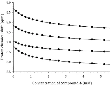
Figure S13: 1H NMR chemical shifts as a function of solute concentration for 4, Proflavine, measured at T = 298 K.
[image:44.595.105.480.41.328.2]S10
Figure S15: 1H NMR-derived diffusion coefficient as a function of solute concentration for 4, Proflavine, at T = 298 K.
[image:45.595.109.480.406.678.2]