A model of meta-population dynamics for North Sea and West of Scotland cod - the dynamic consequences of natal fidelity

A model of meta-population dynamics for North Sea and West of Scotland

cod—The dynamic consequences of natal fidelity

Michael R. Heath

_{, Philip A. Kunzlik, Alejandro Gallego, Steven J. Holmes, Peter J. Wright}

FRS Marine Laboratory, 375 Victoria Road, Aberdeen AB11 9DB, UK

a r t i c l e

i n f o

Keywords: North Sea cod Migration Genetics Spatial modelling Population structure

a b s t r a c t

It is clear from a variety of data that cod (Gadus morhua) in the North Sea do not constitute a homo-geneous population that will rapidly redistribute in response to local variability in exploitation. Hence, local exploitation has the potential to deplete local populations, perhaps to the extent that depensation occurs and recovery is impossible without recolonisation from other areas, with consequent loss of genetic diversity. The oceanographic, biological and behavioural processes which maintain the spatial population structures are only partly understood, and one of the key unknown factors is the extent to which cod exhibit homing migrations to natal spawning areas. Here, we describe a model comprising 10 interlinked demes of cod in European waters, each representing groups of fish with a common natal origin. The spawn-ing locations of fish in each deme are governed by a variety of rules concernspawn-ing oceanographic dispersal, migration behaviour and straying. We describe numerical experiments with the model and comparisons with observations, which lead us to conclude that active homing is probably not necessary to explain some of the population structures of European cod. Separation of some sub-populations is possible through dis-tance and oceanographic processes affecting the dispersal of eggs and larvae. However, other evidence suggests that homing may be a necessary behaviour to explain the structure of other sub-populations. The consequences for fisheries management of taking into account spatial population structuring are compli-cated. For example, recovery or recolonisation strategies require consideration not only of mortality rates in the target area for restoration, but also in the source areas for the recruits which may be far removed depending on the oceanography. The model has an inbuilt capability to address issues concerning the effects of climate change, including temperature change, on spatial patterns of recruitment, development and population structure in cod.

1. Introduction

Cod (Gadus morhua) stocks across the entire geographic range in the North Atlantic were subjected to intense fishing pressure during the 20th century and many suffered well-documented col-lapses. Subsequent analyses have shown that in some outstanding cases, e.g. the northern cod stock off Newfoundland, the terminal collapse was probably due to a combination of over-fishing and adverse climate (Rose, 2004). In this case, even a total cessation of fishing does not seem to have promoted recovery.

It is feared that a similar train of events to those seen off New-foundland may be taking place in European waters. The high fishing mortality rates that developed following the so-called gadoid out-burst (Cushing, 1984), a period of high productivity for gadoids in the 1960s and 1970s, were considered unsustainable by the early

∗_{Corresponding author. Tel.: +44 1224 876544; fax: +44 1224 295511.} E-mail address:heathmr@marlab.ac.uk(M.R. Heath).

1990s. However, the gap between actual and sustainable exploita-tion rates continued to widen (Cook et al., 1997), exacerbated by a decline in productivity linked to climate change. In the case of the North Sea, the climatic link is manifest as a negative correla-tion between recruitment and sea temperature, which is in turn linked to the North Atlantic Oscillation Index (Beaugrand et al., 2003; Brander and Mohn, 2004; O’Brien et al., 2000; Planque and Fr ´edou, 1999). Starting in 2000, various cod stock recovery mea-sures were enacted with the specific aim of allowing as many cod as possible to spawn (Anon., 2000, 2001). ICES finally recommended a total cessation of fishing for cod in certain areas in 2002 (ICES, 2003).

commensu-rate reduction in the total allowable catches of cod. Subsequently, enhanced opportunities to fish for other demersal species were permitted in areas and at times when cod historically constituted a small proportion of the demersal fish assemblage. However, it has long been suspected that cod is a population rich species with complex spatial structure (Sinclair, 1988), and since all of the opera-tional models of North Sea cod were based on whole-stock spatially aggregated dynamics, it was hypothesised that prognoses of the likely impact of spatially structured regulations could, at best, be considered to be only very approximate.

Fishermen have known for centuries that cod migrate annu-ally to particular locations to spawn (Kurlansky, 1999), and tagging studies from across the North Atlantic indicate a high degree of spawning site fidelity among repeat-spawning fish. A high pro-portion of fish tagged on a spawning site at spawning time and recovered at spawning time in subsequent years are recovered within a short radius of their original tagging location, whilst recov-eries at other times of year may have moved considerable distances (Robichaud and Rose, 2001, 2004; Wright et al., 2006a). At the same time, it is clear that there are regional differences in demography and phenotypic properties of fish, which seem to be related to the different spawning regions (West, 1970; Yoneda and Wright, 2004; Olsen et al., 2004; Galley et al., 2006; Wright et al., 2006b). The impression is that cod may exhibit a meta-population structure comprising sub-populations with low rates of inter-mixing due to the passive transport of eggs and larvae, and straying of juveniles and adults.

Tagging studies cannot give insight on the extent to which apparently distinct spawning populations may be reproductively isolated, i.e. whether the return migration of adults to particular spawning sites represents natal fidelity. Early attempts at allozyme based genetic studies indicated that, in the North Sea, cod were a single panmictic unit (Jamieson and Thompson, 1972; Child, 1988). However, more recently,Hutchinson et al. (2001) inves-tigated microsatellite DNA markers and found four genetically distinct groups centred on Bergen Bank, Moray Firth, Flambor-ough Head and the Southern Bight (Fig. 1), which broadly map onto combinations of the groupings emerging from tagging and otolith shape studies (Wright et al., 2006a; Righton et al., 2007; Galley et al., 2006). Differentiation was weak but significant, and the degree of genetic isolation was weakly correlated with the geo-graphical separation distance. Hence, the implication was that the cycle of spawning, larval drift, juvenile and adult migration is self-contained over the geographical scale of each of these groups of spawning areas, with relatively little straying. Long-term changes (1954–1998) in genetic structuring have also been examined by DNA analysis of archived otoliths from the Flamborough Head pop-ulation (Hutchinson et al., 2003). These data indicated marked genetic changes and loss of allelic diversity during a period of sig-nificant decline in abundance.

The key conclusion from the combination of tagging, genetic, microchemistry and morphometric studies on cod in European waters is that the essential spatial scale of breeding populations is smaller than the current stock assessment units, and is defined by some function of larval drift and juvenile and adult migra-tion patterns. As a consequence, recovery plans involving spatially structured fishery regulations may have unforeseen outcomes depending on their placement, and any benefits may not be dis-tributed equally over the current assessment regions.

Our objective in this study was to examine the consequences of different assumptions about natal fidelity for regional dynamics and population structuring. Hence we required to track the devel-opment of genetic populations. To achieve this we developed a model which represented multiple demes by means of age-based discrete time methodology, with a spatial representation of the

physical oceanographic and fish behaviour patterns that maintain spatial organisation, as well as the spatial patterns of production (recruitment and growth) and mortality (natural and fishing). This type of modelling represents a significant departure from the cur-rent modelling approaches as applied to fish stocks.

2. Methods

2.1. Model description

The domain of our model was a subset of the region covered by the annual ICES stock assessments of the North Sea, Skagerrak and eastern Channel (ICES Divisions IIIa (Skagerrak), IV & VIId) and west of Scotland (Division VIa); namely the North Sea and west of Scotland (Divisions IV and VIa). Based on tagging data, geographi-cal distributions of fish from surveys and landings, and studies of fish morphology and microchemistry (Wright et al., 2003, 2006b; Metcalfe et al., 2005; Galley et al., 2006) we identified 10 potentially distinct groupings, or sub-stock units of cod in this region, each associated with a geographically fixed spawning area. Our model was configured to represent each of these (Fig. 1). ICES Divisions IIIa (Skagerrak) and VIId were not explicitly included in this analysis although implicitly Division VIId is incorporated in area 10 (Dogger Bank/Southern Bight) and Division IIIa (Skagerrak) is incorporated in area 8 (Fisher Bank).

The fish in each sub-stock unit were defined as having all been born in the same spawning sub-area of the model domain. Hence, we refer to the sub-stock units as natal populations, and to their associated sub-areas of origin as natal areas. However, there was no requirement in the model that fish should necessarily return to spawn in their natal area, although this was a structural option, so that the group of fish spawning in a sub-area could in principle be composed of fish from a variety of natal populations. But, the offspring of all fish spawning in a sub-area belonged to the ‘local’ natal population for the rest of their lives, regardless of the natal origin of the parents or where they subsequently spawned as adults. Straying, and the processes which might influence straying, were therefore key structural aspects of the system. Hence, the model tracked annual cohorts of fish of distinct geographic origin, and was capable of simulating the proportion of fish spawning in an area which were themselves of local origin. The model could therefore provide an assessment of the scope for genetic isolation, subject to a range of alternative interpretations of the processes controlling migration and interaction between sub-stocks.

Within each natal area we identified firstly, a set of 1/4◦

lati-tude×1/2◦longitude rectangles representing cod spawning areas, on the basis of egg survey data and catches of spawning fish, and secondly a set of rectangles representing suitable nursery habi-tat for juvenile cod based on trawl survey data (Fig. 1). Rectangles recorded as containing either >2 cod eggs m−2_{in plankton surveys,} or >1 spawning fish per hour in trawl surveys were designated as spawning sites. Similarly, rectangles in which age 1 concentrations of cod≥0.01 m−2_{were encountered at any time during annual trawl} surveys in February, were designated as nursery sites into which pelagic juveniles could settle.

2.2. Population dynamics

Fig. 1.Maps of natal areas, spawning and nursery areas. In the left-hand panel, numbers indicate the natal areas delineated by the black outlines: (1) Clyde, (2) West coast, (3) Minches and north coast, (4) Shetland, (5) Viking/Bergen Banks, (6) Moray Firth, (7) East coast, (8) Fisher, (9) Flamborough, (10) Dogger Bank and Southern Bight. Bathymetric contours shown at 200 m (thick grey) and 50 m (thin grey). Dark grey shaded rectangles indicate cells denoted as spawning areas (left panel) or nursery areas (right panel).

each annual age class (a, whereawas an integer between 0 and 20) was further divided into mature (Nmature) and immature (Nimmature), and their numbers updated at monthly intervals (m =0–12, where 0 denotes 1 January, 1 denotes 31 January, and 12 denotes 31 Decem-ber) through each calendar year (y) according to the total mortality rate (Z= natural mortality (M) + fishing mortality (F), month−1_). Natural mortality was applied from the age of transition between drifting larval phase and settled juvenile (recruitment) onwards. Fishing mortality was a prescribed value depending on year and age, and also on month and geographical location. Within each natal population, fish were potentially distributed across any number (up toP) of the nursery, spawning area and feeding areas depending on time of year, larval drift patterns, and post-settlement migration behaviours.

For mature fish in a given natal population (n) and destined to spawn in a given spawning area (j= 1–P), at each time step:

Nmature_{(n,y,m,a j)}=exp(ln(Nmature_n,y,m−1,a j−Mmaturen,y,m,a−Fy,a,m,j))

The natural mortality rateMmaturey,m,awas a continuous function of body length during the monthm(seeAppendix A). The fishing mortality rateFy,a,m,jdepended on year (y), age (a), month (m) and

which spawning area (j) the fish were associated. For immature fish:

Nimmature_(n,y,m,a,c) =exp(ln(Nimmaturen,y,m−1,a,c−Mimmaturen,y,m,a,c

−Fy,a,m,c))

wherecdenoted the nursery areas (c= 1–P). The natural mortal-ity rateMimmaturey,m,a,c was a continuous function of body length during the monthm, as for the mortality rate of mature fish, but additionally included a nursery area specific dependent density dependent component (seeAppendix A).

The total number of fish at age in the natal population was then given by:

Nn,y,m,a= j=P

j=1

Nmature_{n,y,m,a j}+ c=P

c=1

Nimmaturen,y,m,a,c

At the end of each calendar year (m= 12) all the fish in each age class were transferred to the initial conditions (m= 0) for next oldest age class. The first age class (a= 0) was thus vacated, pending recruitment of the young-of-the-year on a given date, and all fish in the oldest class (a= 20) were killed off. During the transfer to next oldest age class, a proportion of immature fish were transferred to the mature state, according to the change in proportion mature at age (Qn,y,a) in the natal population resulting from the increment in

age.Qn,y,awas a function of body length on 1 January each year (see

Appendix A):

Nimmature_n,y,m=0,a,c=Nimmaturen,y−1,m=12,a−1,c×ın

whereın= (1−Qn,y,a)/(1−Qn,y−1,a−1) forQn,y−1,a−1< 1 andın= 0 for

Qn,y−1,a−1= 1

j=P

j=1

Nmature_n,y,m=0,a j = j=P

j=1

Nmature_n,y−1,m=12,a−1j

+ c=P

c=1

(Nimmature_n,y−1,m=12,a−1,c×ı

′

n)

where ı′

n=(Qn,y,a−Qn,y−1,a−1)/(1−Qn,y−1,a−1) for Qn,y−1,a−1< 1 andNimmature_n,y−1,m=12,a−1,c×ı

′

n=0 forQn,y−1,a−1= 1.

later, but briefly, they assigned the area of next spawning on the basis of spawning or nursery area assignment in the previous year.

2.3. Recruitment

Fish were recruited to the first age class (a= 0) of each natal population on a fixed date each year (1 August,m= 8), representing the timing of settlement of pelagic phase juveniles to the demer-sal habitat in each nursery area. The number of fish recruiting to each natal population was determined from the annual population fecundity of all the fish spawning in each spawning area (equivalent to the annual egg production, seeAppendix A), and the proportion of these eggs surviving the drift from release to settlement in each nursery area. This proportion was simulated by an off-line particle-tracking model which modelled the dispersal, growth and survival of eggs and larvae, subject to the year-specific ocean circulation and temperature conditions. For each natal population, the number of potential recruits was then the sum of surviving pelagic juvenile numbers arriving at all nursery areas on settlement date. However, the actual number recruiting to the age-structured natal popula-tion from each nursery area was reduced by a settlement mortality term representing competition for resources in the nursery area. This increased as a function of the total number of juveniles of all natal origins attempting to settle at each nursery area. Thus, the settlement mortality introduced a density dependence acting both within and between natal populations (seeAppendix A).

2.4. Development

The body length of fish was updated at monthly intervals, coin-cident with the updating of per capita abundance. The change in body length over time was represented by the von Bertalanffy growth equation (von Bertalanffy, 1938). All fish in an annual cohort of a natal population inherited the same von Bertalanffy growth parameters which they retained throughout life, regardless of their subsequent migrations. The characteristic growth parameters of fish in each natal population were determined principally from analysis of length and age data collected during annual trawl sur-veys (seeAppendix A).

The proportional distribution between immature and mature state, which was updated annually on 1 January, depended on a continuous function of body length (seeAppendix A). For mature fish, female fecundity was also a continuous function of body length (seeAppendix A).

2.5. Migration

We represented four types of fish movement in the model: (1) passive drift of eggs and larvae, (2) “first-spawning migration” of virgin fish to their first spawning site, (3) annual migration of mature fish between spawning sites and a summer feeding area, and (4) straying of repeat spawning fish from their area of first spawning to other spawning areas (Fig. 2).

Whilst spawning site fidelity of repeat spawning fish and seasonal migrations of adult cod were relatively easily inferred from tagging data, there were few data for inferring migrations of juveniles and no basis for determining the extent of natal fidelity involved in spawning site selection by fish. Spawning site fidelity of repeat spawning fish was therefore parameterised in the model on the basis of tagging data, but alternative views of first-spawning migrations and natal fidelity were treated as structural variants of the model (Fig. 2). In reality, these vari-ants might not be mutually exclusive in their representation of first-spawning migration behaviours across the model region, but their performance relative to our understanding of the spatial

Fig. 2.Schematic of drift and migration connections between areas occupied by fish in different life stages. Upper panel: connections between nursery, spawning and adult feeding areas, illustrated by an example of two spawning and nursery areas, with a single shared feeding area. Shading patterns denote nursery, spawn-ing, feedspawn-ing, and sink areas for eggs and larvae. Arrows show movements of fish from source to destination areas due to egg and larval drift, first-spawning migra-tion, and repeat spawner migration. Lower three panels illustrate the connections between three spawning and nursery areas for different structural variants of the model representing scenarios of first-spawning migration behaviour denoted by ‘homing’, ‘oceanography’ and ‘diffusion’. In these panels the positioning of spawning and nursery areas is indicative of spatial proximities. Shading and arrow patterns as in the upper panel (open circles, nursery areas; grey shaded circles, spawning areas; dashed arrows, egg and larval drift; grey arrows, first-spawning migration). Note that the pattern of egg and larval drift is the same in each case, but in the homing scenario first-time spawners return to their natal spawning ground. In the oceanography sce-nario first-time spawners remain at the spawning area closest to their nursery area regardless of natal origin. In the diffusion scenario, first-time spawners disperse to spawning areas adjoining their nursery area regardless of natal origin.

dynamics of abundance was a key aspect of the analysis of the model.

2.6. Passive drift

2.7. First-spawning migration

The juveniles in each nursery area were assigned a future spawn-ing affiliation to represent their eventual first-spawnspawn-ing migration. This assignment was one of the key structural variants in the model (Fig. 2) and the consequences for the overall population dynamics of varying the degree of natal spawning fidelity was one of the fea-tures of the model which we wished to explore. The proportions of individuals in each natal population at each nursery area des-tined to spawn at each spawning area (Vn,c,j,

=P

c=1Vn,c,j=1) were set to mimic one of three first-spawning migration scenarios. In the first scenario, which we refer to as the ‘homing scenario’, all fish migrated to their spawning area of origin to spawn for the first time. Thus first spawning fish were faithful to their natal origin. In the second scenario, which we refer to as the ‘oceanography sce-nario’, the future first spawning area assignment of juveniles was set to equal their nursery area regardless of their origins. Thus, in this scenario the distribution of first spawning fish within a natal population was dictated solely by ocean circulation. In the third scenario, which we refer to as the ‘diffusion scenario’, a proportion of fish in each nursery area emigrated to adjoining areas to spawn for the first time. The remainder behaved as in the oceanography scenario. For those fish that emigrated in the diffusion scenario, the distribution across destination spawning areas was determined from the proportion of source nursery area boundary in common with each destination spawning area. The proportion emigrating from the nursery area (pm) was treated as a sensitivity testing parameter. Thus, there was scope for cross-breeding between natal populations among first-time spawners in the oceanography and diffusion scenarios, depending on oceanographic dispersal and the emigration parameter pm, but not in the homing scenario.

2.8. Annual migration

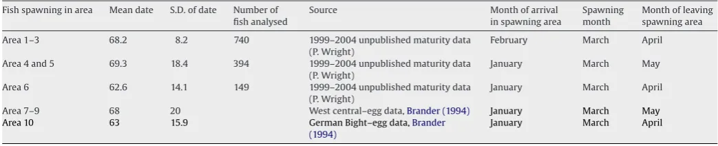
We simplified the annual migration behaviour of mature fish by specifying that they spend a fixed proportion of each year of mature life in the vicinity of a chosen set of spawning rectangles, and the remainder of the year feeding elsewhere. The timing of migrations between spawning and feeding areas varied between spawning areas, and was estimated from the mean and standard deviation of spawning date in each natal area. Spawning dates were derived from a combination of the recorded dates of capture of maturity states of female cod (areas 1–6) (see methodology ofHeath and Gallego, 1998), and egg survey data published byBrander (1994) (areas 7–10) (Table 1). The duration of residency in the spawn-ing area was taken to be 6 standard deviations around the mean spawning date.

2.9. Straying of repeat spawners

Subsequent to first spawning, fish were allowed to change their spawning affiliation on an annual basis to mimic the straying

pat-terns revealed by tagging data. This straying was independent of natal population and represented the accuracy with which fish returned to the same spawning site each year, not the fidelity of fish to their natal origin. A matrix (Sa,j-previous,j-next) specified the proportion of mature fish of age a which, having spawned in area j-previous in the current year, will spawn in areaj-next in the fol-lowing year. Hence, for each value ofaandj-current,

j-next=P

j-next=1

S(a,j-previous,j-next)=1

Spawning area affiliations were assigned on 1 January each year, in advance of the first appearance of fish in any of the spawning areas.

The matrixSwas parameterised with data on the recapture loca-tions of fish tagged during spawning months (January–April) and retrieved during the same period in subsequent years. Data and methods for standardising tag recoveries for catch rates in the fish-ery are given inWright et al. (2006a). A2_{-test was used to test the} null hypothesis that there is no difference between age classes in the proportion of fish tagged in one area and recovered from other areas. The average stray proportion (ps) was used to calculate the expected frequency for each age.

2.10. Spatial and temporal distribution of fishing mortality

Estimating spatial and temporal variability in the fishing mor-tality rate (F) on cod is highly problematic. For the North Sea and west of Scotland, where the fishery is multi-species and conducted by a variety of fleets from a variety of nations, reliable spatially resolved data on effort are extremely difficult to compile, and in any case are not simply related to mortality rates. Landings data are more readily available, but also not easily related to mortality. Hence, we analysed trawl survey data collected in February/March each year to estimate the total mortality of age classes between successive annual surveys, and used these to apportion the ICES regional fishing mortality rates between our model areas.

The ICES stock assessments provide year-by-year hindcasts of the regional scale annual averaged fishing mortality in the North Sea (ICES areas IIIa (Skagerrak), IV and VIId) and west of Scotland (ICES area VIa) for each age class of cod (ICES, 2005, 2006). We used 1980–1999 mean fishing mortality rates at age from the versions of the ICES assessments which included discards in the catch records, or scaled multiples of these, as the basis for setting the absolute level of mortality in our simulations, and developed temporal and spatial scaling on the basis of landings and survey data. The assess-ment outputs provide fishing mortality rates up to age 6 (age 7 for area VIa), so we assumed a constant fishing mortality rate over all older age classes.

For each region (R) (R = “west of Scotland” for model areas 1–3, R = “North Sea” for model areas 4–10), the ICES annual

fish-Table 1

Summary of data used to assign spawning months to fish in each natal population

Fish spawning in area Mean date S.D. of date Number of fish analysed

Source Month of arrival in spawning area

Spawning month

Month of leaving spawning area

Area 1–3 68.2 8.2 740 1999–2004 unpublished maturity data (P. Wright)

February March April

Area 4 and 5 69.3 18.4 394 1999–2004 unpublished maturity data (P. Wright)

January March May

Area 6 62.6 14.1 149 1999–2004 unpublished maturity data (P. Wright)

January March April

Area 7–9 68 20 West central–egg data,Brander (1994) January March May

Area 10 63 15.9 German Bight–egg data,Brander

(1994)

ing mortality rate by age class, averaged over 1980–1999, was first expressed as a monthly rate (Fmonthly=Fannual/12). For the mature age classes, the temporal distribution of the regional fish-ing mortality (ICESFa,R) between the period of the year spent in the spawning areas ((ICESFa,R)spawning) and the period spent on feeding grounds ((ICESFa,R)feeding), was apportioned according to the temporal distribution of landings, such that the annual average rate corresponded with that from the assessments. For immature fish the regional rate of fishing mortality was assumed to apply throughout the year.

Spatial variations in fishing mortality on mature fish during the feeding period of the year were not resolved in the model. All mature fish associated with spawning areas 1–3 were subjected to the feeding period rate of mortality corresponding to the west of Scotland assessment, and mature fish associated with areas 4–10 were subjected to the North Sea regional rate during the feeding period. However, the spawning period rates of fishing mortality in the North Sea and west of Scotland regions ((ICESFa,R)spawning) were further resolved to spatial areas according to catch rates from trawl surveys. Similarly, fishing mortality on immature fish was resolved to spatial areas.

Each February since 1983, the ICES International Bottom Trawl (IBTS) survey of the North Sea has sampled fish by means of stan-dardised tows with the GOV trawl from an international fleet of survey vessels. Individual lengths of catches of all species are mea-sured at sea and ages of key species determined by length stratified sub-sampling for otoliths. Data on catch per unit effort (CPUE, num-bers h−1_{) at age (a) of cod in each sampling tow in the North Sea} were obtained for years (y) 1983–2004 from the ICES data centre. An equivalent survey of the west of Scotland region (ICES area VI) is carried out in March each year, immediately following the IBTS, and these data (1985–2004) were available at the Marine Labora-tory Aberdeen. CPUE at age in each survey year from both surveys was spatially averaged over each of our 10 model areas (J), accord-ing to the locations of each tow to give an estimate of density. The methodology for spatial averaging has been described byHolmes et al. (2008).

For each of the 10 areas we estimated the average over the survey series of age-specific total mortality rate (Za,J, y−1) in each of our

model sub-areas:

Za,J=ln(CPUEy+1,a+1,J)−ln(CPUEy,a,J)

where CPUEy,a,Jwas the area averaged catch per unit effort in yeary

of age a in areaJ. Assuming that age-specific natural mortality (M) does not vary systematically between sub-areas, we then scaled the age-specific total mortality rates for each area to represent fish-ing mortality rates (F=Z−M), such that after abundance weighting each value, the average over each ICES assessment regions (R) equalled the corresponding regional fishing mortality rate. Weight-ing factors for mature and immature mortality rate were calculated on the basis of the mean averaged CPUE for specific age classes over the each of the survey series:

mature,R

=

J=1((Za=3 to 5,J·CPUEa=4,J·ssaJ)/((

J=1CPUEa=4,J·ssaJ)/P)) P

immature,R

=

J=1((Za=2 to 3,J·CPUEa=2,J·ssaJ)/((

J=1CPUEa=2,J·ssaJ)/P)) P

where ssaJwas the sea surface area of areaJ,J= 1–3 for R = ICES

area VI, andJ= 4–10 for R = ICES area IV. The age groups chosen to represent mature and immature fish reflected the maturation rates in the model. In the slowest growing natal population, 45% of females were mature at age 3, and 85% in the fastest growing population. Then, for mature fish during the spawning months of the year,

Fa,m,j=

Za=3 to 5,J·(ICESFa,R)spawning mature,R

where ((ICESFa,R)spawning) represents the regional (R) age-specific fishing mortality rate during the spawning months averaged over 1980–1999 from the annual ICES stock assessment analyses. For immature fish throughout the year,

Fa,m,c=Za=2 to 3,J

·(ICESFa,R)

immature,R

2.11. Initial conditions

Initial conditions (numbers at age on 1 January in a given year in each natal population, their distributions across nursery areas and assignments to spawning areas) were derived from a combination of trawl survey data and the annual ICES cod stock assessments for regions VI and IV (west of Scotland and North Sea respectively). The regional assessment numbers at age were distributed across the 10 model areas, in proportion to the area-specific CPUE from the trawl February/March trawl surveys. As an initial state for the model, we assumed that all the immature and mature fish in a given area were drawn from the same, local natal population.

2.12. Output

The mode of operation of the model was to first select one of the alternative scenarios of first-spawning migration (oceanography, homing or diffusion), repeat spawner straying enabled or disabled, and then a specific year to represent initial conditions of population age structure and abundance, regional fishing mortality rate, ocean circulation and temperature climatology. Regardless of the config-uration selected, the model was then run to a stationary state with a repeating annual cycle of climatology and fishing mortality rates. Fishing mortality rates were varied by applying a scaling fac-tor (F) to the ICES regional estimates of fishing mortality at age (ICESFa,R). Each simulation year, the programme output the total numbers of fish at age on 1 January for each natal population, and the proportions of each age class and natal population asso-ciated with each spawning and nursery area. These data were then summarised by calculating the spawning stock biomass (SSB) and recruitment for each natal population and spawning group of fish. SSB referred to males and females combined, and was calculated as the sum over each age, natal population and spawning area of the product of mature numbers at age and weight at age:

SSBn,y,m,j= a=20

a=0

(Nmature×Wtn,y,a)

be the progeny of the spawning stock in that area. In the homing scenario, this definition of recruitment matched the number of age 1 fish in each of the natal populations. In the oceanography sce-nario recruitment to a spawning group was then the number of age 1 fish in the nursery area local to each spawning area. In the dif-fusion scenario, spawning group recruitment was the sum over all nursery areas of the age 1 fish which, if they survived, on attaining maturity would be assigned to a given spawning area, based on the emigration rate parameter and emigration pattern defined for the scenario.

2.13. Calibration data

We calibrated key model parameters by exploring a range of values and selecting a combination which resulted in equivalent properties of the relationship between regionally integrated SSB and recruitment simulated by the model, and that derived from the ICES regional stock assessments for cod. Of the two relevant regional stock assessments (R = “west of Scotland” (ICES area VI) for model areas 1–3, R = “North Sea” (ICES area IV) for model areas 4–10), that for the North Sea has been subject to more critical review and evaluation, and was the main focus for our calibration effort. The west of Scotland assessment data are viewed as being more uncertain due to the smaller population size, poorer survey indices, less well documented catch data and less refinement of natural mortality values in the catch-at-age analysis.

The underlying relationship between SSB and recruitment is tra-ditionally derived from a time series of fish stock demographic data by fitting a Ricker function (Ricker, 1975), or similar functional rela-tionship, to the set of paired values of recruitment (y) and SSB in the year in which the recruits were spawned (x). However, a key condition of this approach is that residuals between observed and fitted recruitment at a given SSB should be random with respect to time. If this condition is not met then it is unlikely that the fit-ted relationship can reflect the underlying biology in a meaningful way. The most likely cause of non-randomness with respect to time would be some relationship between survival and environmental factors which vary systematically over time. In the case of North Sea cod, there is a well documented relationship between Ricker-residuals and temperature, so it was necessary for us to resolve at least this component of variability and reference the underlying SSB:recruitment relationship to the temperature regime over the period represented by our model runs.

We fitted, by Simplex optimisation, a modified Ricker model (referred to as T-Ricker) incorporating a temperature term, as described byStocker et al.(1985),Planque and Fr ´edou (1999),Clarke et al. (2003)andCook and Heath (2005):

Recruitment=b·SSB e(d·T−SSB/f)

whereb,dandfare fitting parameters.

The temperature index (T) was as described byCook and Heath (2005), i.e. the results from a factor analysis of time series of temperature at 10 locations in the North Sea, equivalent to the first component of a principal components analysis. To check for unresolved systematic time-dependent structure in residuals, we plotted log-residuals (ln(observed recruitment)−ln (fitted recruit-ment)) against time (year), and fitted a Local Polynomial Regression (LOESS) smoother with a span of 0.37 (n= 41) and tricubic weighting (Cleveland et al., 1992) using the package R (R Core Development Team, 2005). Where the results showed systematic deviations from zero with time, the smoothed residuals were added back to the fit-ted recruitment from theT-Ricker function, on a year-by-year basis. Hence the pairs of observations of SSB and recruitment contained in the assessment time series could be considered as point

sam-Table 2

Spawning biomass thresholds for defining effective extinction of natal populations or spawning groups in each model area

Area Threshold SSB (tonnes)

1 43.5

2 99.5

3 230.0

4 96.0

5 527.8

6 112.0

7 96.0

8 767.7

9 128.0

10 799.7

The thresholds were set as 1% of the maximum observed regional SSB for west of Scotland (areas 1–3) and North Sea (areas 4–10) distributed such as to assume uniform area density.

ples from a family of year-specific stock:recruitment relationships, each of which was unique depending on the prevailing tempera-ture and other environmental condition represented by the value of time-dependent LOESS smooth. To visualise each of these year-specific relationships, we derived recruitment values for a sequence of values of SSB in the range 0–300,000 tonnes, from the combina-tion of year-specific temperature and the fittedT-Ricker equation, and year-specific values of the LOESS smoothed residuals. Statistics (median and centiles) of the underlying relationship could then be estimated over any given period of years, and these formed the basis for our calibration data for comparing with the model results.

2.14. Characterisation of sub-stock richness and evenness

We defined two indices to describe the richness and evenness of sub-stocks in the model, based on the Shannon–Wiener diversity index (Magurran, 1988; Sokal and Rohlf, 1995). Sub-stock richness was defined as ln(P*) whereP*was the number of extant natal popu-lations or occupied spawning areas in the simulation. The evenness of extant populations was then given byeSW/P*_{where SW was the} Shannon–Wiener diversity index:

SW=

J=P∗

J=1

Jln(J) where J= SSBJ

J=1SSBJ

High values of the evenness index corresponded to distributions which were more clumped or aggregated into a few areas, whilst low values indicated that biomass was more uniformly distributed. We set biomass thresholds as criteria for assessing whether a natal population or spawning group was either ‘collapsed’ or ‘effectively extinct’, and hence for their inclusion in the richness and evenness indices. We arbitrarily chose 1% of the maximum observed regional SSB for the west of Scotland (37,295 tonnes) and North Sea (252,712 tonnes) as being appropriate regional thresh-olds to delineate effective extinction (i.e. 373 tonnes for west of Scotland and 2527 tonnes for the North Sea). Similarly we chose 4% of the maximum observed regional SSB as being indicative of collapse. In each case, we distributed these regional thresh-old SSB values across the model areas so as to assume equal area population-density over spawning areas 1–3 and 4–10 (Table 2).

3. Results

3.1. Patterns in the driving data of the model

Fig. 3.Average (1985–2004) values of area-integrated CPUE in each model sub-area from the trawl surveys in February/March.

Fig. 4.Mean age-specific total mortality in each of the model areas (ZJ,a).

shown inFig. 3. The means of age-specific total mortality in each of the model areas (ZJ,a) implied by these data are shown inFig. 4.

Applying these data to dis-aggregate the ICES estimates of region-ally averaged fishing mortality resulted in the spawning period rates of fishing mortality, and fishing mortalities on juveniles indi-cated inFig. 5.

3.2. Straying rate of adult fish

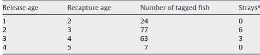
There were 363 records of fish having been tagged in model areas at spawning time and recaptured during spawning times in subsequent years. Of these a proportion had no associated data on the age of the fish. The Moray Firth (area 6) had the largest number of releases and recaptures, with 171 aged records of use to this study. The average proportion straying for all ages was 0.053 (Table 3). The2_{= 2.22 which is <}2 _{at P= 0.05 of 7.815.} There-fore, the null hypothesis that there was no difference between age classes in the proportion of fish straying to other areas could not be rejected.

The standardised straying rates (proportion of tags of all ages recovered from sink areas, i.e. areas other than that in which fish

Table 3

Frequency of tag recaptures and strays outside tagging regions

Release age Recapture age Number of tagged fish Straysa

1 2 24 0

2 3 77 6

3 4 63 3

4 5 7 0

a_{Before standardization.}

Table 4

Proportion of fish tagged at spawning time in areas 1, 3 and 6 which were recaptured from various areas at spawning time in subsequent years

Recapture area Release area

1 3a ₆

1 0.995 0.030 0

2 0 0 0

3 0 0.894 0.050

4 0 0.036 0.003

5 0 0 0

6 0 0.034 0.947

7 0.005 0.006 0

a_{Region based on standardised recoveries from two release sites.}

were released) are given inTable 4. The data covered too few source areas to justify defining source specific straying rates. On the basis of the results, we assumed that the straying rate of repeat spawning fish was 5% for each source area. Sink areas were assumed to be all adjoining areas, and the strays were spread evenly across each of the sinks.

3.3. Dispersal and survival patterns of eggs and larvae

Averaged over all years between 1980 and 1999, a high propor-tion of simulated drift tracks led to sites of suitable nursery habitat from spawning locations in the southern and western North Sea (areas 6–10), and in the southern North Sea (areas 8–10) tracks were retained within the area of origin (Fig. 6). However, a lower

Fig. 6.1980–1999 average results from the biophysical model of egg and larval dispersal and survival. Upper panels: to the left, colour shading indicates the average proportion of drift tracks starting in each spawning area (rows) which terminate as a 35 mm larva within a given nursery area (columns). Grey filled cells indicate that there was no drift of eggs and larvae between the given spawning and nursery area. To the right, the bar diagram shows the cumulative total proportion of drift tracks from each spawning area which terminate over nursery areas. Lower panels: to the left, colour shading indicates the average survival (proportion of eggs surviving to become a 35 mm larva) along drift tracks starting in each spawning area (rows) and terminating within a given nursery area (columns). To the right, the bar diagram shows the cumulative total survival for all drift tracks from each spawning area which terminate over nursery areas.

proportion of trajectories led to nursery sites from spawning in the northern North Sea (areas 4 and 5). On the west coast of Scotland, nursery locations were more widely dispersed, and a low propor-tion of trajectories were retained within the area of origin.

Survival rates along trajectories that terminated over suitable nursery habitat showed a rather different pattern (Fig. 6). Tracks leading to settlement at Shetland (area 4) showed the highest sur-vival rates, having originated from widely distributed areas of the west of Scotland and the northern North Sea (areas 1–5). Tracks

ter-minating at nursery sites in the southern North Sea (areas 9 and 10) showed uniformly low survival, having originated from throughout the North Sea and north of Scotland.

Fig. 7.Combined drift and survival probabilities for all tracks leading from spawning areas to nursery areas.

northern North Sea (areas 1–5) (Fig. 7). This proportion showed a significant (p< 0.05) increasing trend over time (1980–1999) for areas 8 and 10 in the southern North Sea, but no significant trend in other areas.

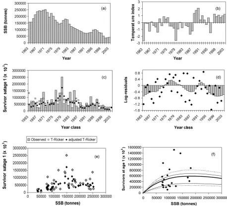
3.4. North Sea regional stock:recruitment relationship

Time series of SSB and recruitment from the ICES regional assessment of the North Sea, and the North Sea temperature index are shown inFig. 8. Fitting of the temperature dependent Ricker model accounted for 34% of the variance in recruitment (Fig. 8). There was no relationship between residuals from the fitted model and SSB, indicating that the compensatory form of the Ricker model was appropriate for describing the observations. However, the residuals did show strong systematic time dependency (Fig. 8).

Fig. 9.Emergent relationships between equilibrium spawning biomass and recruit-ment, integrated over areas 4–10 (North Sea), for different values of the pelagic survival-scaling factorϕ. Panels correspond to each of the three scenarios of first-spawning migration. Model data are compared to the median, 17th and 83rd centiles of the family of stock-recruitment relationships for the years 1980–1999 (fromFig. 8).

When the LOESS smooth with respect to time of these residuals was added back to the Ricker fitted values, the resulting combined estimate accounted for an increased 46% of the variance in the observations.

The median, 17th and 83rd centiles of the family of year-specific stock:recruitment relationships over the period 1980–1999 (corresponding to the years included in the dispersal and sur-vival estimates from the bio-physical particle-tracking model), are shown inFig. 8. These formed the basis for calibration of the pelagic survival parameterϕ(see below).

3.5. Model calibration and regional parameter sensitivity

The pelagic survival estimated by the bio-physical model can only be regarded as a relative index between each combina-tion of spawning and nursery areas. In order to estimate an appropriate value for the pelagic survival scaling factor (ϕ), we sim-ulated values of spawning biomass (SSB) and numbers of recruits (age 1 on 1 January) in each natal population, for a matrix of

Fig. 10. Equilibrium spawning biomass (SSB) summed over spawning groups in areas 4–10 (North Sea, upper panel), and 1–3 (west of Scotland, lower panel), related to the regional rate of fishing mortality over ages 3–7 in the model. Lines represent different first-spawning migration scenarios according to the legends. Filled trian-gles represent the observations of SSB and age 3–7 fishing mortality rate from the corresponding ICES stock assessments.

scaling values of fishing mortality (F) and values of ϕ. Val-ues close to the equilibrium solution were generally obtained within 75 simulation years. For any given value of ϕ, the equi-librium SSB and numbers of recruits (taken as the results after 200 simulation years) were indirectly related to the fishing mor-tality scaling factor. Low values of ϕcombined with high values of fishing mortality resulted in collapse of the entire regional population.

Fig. 11.Natal purity (left column) and fidelity (right column) for each spawning group, in relation to fishing mortality scaling and first-spawning migration scenario. Natal purity was the Shannon–Wiener based evenness index calculated on the proportion of equilibrium SSB in each spawning group contr buted by each natal population. Fidelity was the proportion of equilibrium SSB in each spawning group which was of local natal origin.

3.6. Spatial sensitivity to fishing mortality and first-spawning migration scenarios

The model predicted declining values of regional scale (summed over areas 1–3 and areas 4–10) equilibrium spawning stock biomass with increasing regional fishing mortality rate. The simulated data were compared with the observed time series of SSB and fishing mortality rate from the ICES stock assessments for the West of Scot-land and the North Sea (Fig. 10), though the observed data do not necessarily reflect equilibrium conditions. In the case of the North Sea, the simulated relationship assuming the homing and oceanog-raphy scenarios of first-spawning migration conformed with the observations in that the rate of decline in SSB decreased at high rates of fishing mortality. In contrast, simulations assuming the dif-fusion scenario resulted in a precipitous collapse of SSB as regional fishing mortality rate exceeded 0.9. However, for the West of Scot-land, only the simulations based on the homing scenario bore any relation to the observations. Both the oceanography and diffusion scenarios resulted in precipitous collapses of SSB at modest fishing mortality rates, in contrast with the observations.

Fig. 12.Pairwise estimates of Bray–Curtis dissimilarity between spawning groups based on the contribution of natal populations to the equilibrium SSB, in relation to corresponding pairwise separation distances (km) of the geographic centroids of each area in the model. Panels correspond to results for combinations of fishing mortality scaling factor (0.6 or 1.0) and first-spawning migration scenario.

The scope for genetic isolation of a spawning group was indi-cated, not by the natal purity of spawning fish, but by the proportion of spawners which were of local natal origin (natal fidelity). The relationship between natal purity and natal fidelity in a spawning group was not straightforward. For example, in the diffusion sce-nario, fish spawning in area 1 had a high degree of natal purity, but only 10–20% were of local origin (Fig. 11). Most had been spawned

in area 2. Area 10 consistently showed high natal fidelity regardless of migration scenario, whilst areas 4 and 5 showed consistently low fidelity even in the homing scenario. In the homing and oceanog-raphy scenarios, natal fidelity increased with fishing mortality.

spawn-Fig. 13.Multidimensional scaling (MDS) diagrams showing ‘natal distance’ between spawning groups, denoted by numeric labels, based on the contribution of natal populations to the equilibrium SSB. Panels correspond to results for combinations of fishing mortality scaling factor (0.6 or 1.0) and first-spawning migration scenario. Spawning groups which are closest together in each diagram are the most similar with respect to the natal composition of fish. Groups enclosed by dashed lines are from the extreme southwest of the model domain (areas 1 and 2), whilst those enclosed by a continuous grey line are from the southern North Sea (areas 8, 9 and 10).

ing groups, based on the proportions of SSB contributed by each natal population. We related the coefficients to the geographical distance (km) between the centroids of each pair of areas. To esti-mate the distance between areas in the North Sea and those to the west of Scotland we used the centroids of areas 3 and 4 as ‘stag-ing posts’ to compute the distance around the north of Scotland. The results (Fig. 12) showed very different patterns of spatial

Fig. 14.Upper panel: maximum equilibrium (sustainable) yield (tonnes) for each spawning group under each of the three scenarios of first-spawning migration, together with the maximum yield for the West of Scotland region (sum over spawn-ing groups 1–3) and the North Sea (sum over spawnspawn-ing groups 4–10). Lower panel: fishing mortality rate corresponding to the maximum sustainable yield (FMSY) for each spawning group, and the West of Scotland and North Sea regions. For individual spawning groups the fishing mortality is the local rate for each group.

was only a weak effect of separation distance on dissimilarity at lowF-scaling, and none at highF-scaling. In contrast, separation dis-tance accounted for a high proportion of the dissimilarity between spawning groups under the diffusion scenario at both high and low F-scaling.

To investigate clustering of spawning groups with respect to natal origins, we conducted Multidimensional Scaling (MDS) anal-ysis (Carroll and Arabie, 1980; Kruskal and Wish, 1978) with a Kruskal loss function and log-scaling of the relationship between dissimilarities and distance, based on the proportions of SSB con-tributed by each natal population. In each case (Fig. 13) the first dimension was closely related to the geographical structuring of the spawning areas, and hence reflected the results of the Bray–Curtis analysis. The second dimension reflected other aspects of the natal composition such as the richness and evenness, and was more sen-sitive to fishing mortality. Spawning groups 8, 9 and 10 emerged as being distinctly different from others in the North Sea, regard-less of the assumed migration scenario and fishing mortality. In fact, increasedF-scaling tended to accentuate the distance between these groups and the others especially under the homing and oceanography scenarios.

We extracted data from model runs with different fishing mortality scaling factors to characterise the emergent yield rela-tionships for individual spawning groups. For each spawning group the equilibrium catch (tonnes) showed a characteristic dome shaped relationship with local fishing mortality rate, and under the oceanography and diffusion scenarios, maximum equilibrium (sustainable) yield (MSY) was greatest in areas 8 and 10 (Fisher and Dogger/Southern Bight) (Fig. 14). However, a different pattern

was found when assuming the homing scenario. In this case, area 6 (Moray Firth) was estimated to produce the greatest MSY. Under all scenarios, the North Sea regional MSY (areas 4–10) was approxi-mately 180,000 tonnes, which was in accordance with independent results from spatially integrated yield models (e.g.Cook and Heath, 2005). The fishing mortality rate at MSY (FMSY) clearly varied con-siderably between spawning groups (areas), being >0.5 in areas 3, 5, 8 and 10, and <0.2 in the inshore areas off the east coast of the UK (6 and 7), regardless of the assumed first-spawning migra-tion scenario (Fig. 14). The ambient fishing mortality rates in each area derived by apportioning the 1980–1999 mean ICES regional rates across areas based on survey data (Fig. 5), were all higher than the area specific values ofFMSY. For the western and north-ern areas (1–6),Fambient/FMSYwas between 2.0 and 2.5, whilst for the southern areas this ratio was between 1.0 and 1.6. For areas 4–10 combined (North Sea), the ratioFambient/FMSYwas >2.0 when assuming homing, and in the range 1.3–1.6 assuming the oceanog-raphy or diffusion scenario.

3.7. Recovery scenario analysis

We conducted a scenario analysis of recovery from a collapsed state. Area specific fishing mortalities were scaled such that the North Sea regional rate was 1.0 y−1_{, and the model then run until} half of the spawning groups had declined to less than the threshold for collapse (4% of the maximum observed regional SSB appor-tioned across spawning areas). Fishing mortality rates were then rescaled so that the North Sea regional rate was 0.5 y−1_{and the run} continued.

The time from the start of each run until 50% of the spawning groups had collapsed varied depending on the assumed first-spawning migration scenario (homing, 29 years; oceanography, 30 years; diffusion, 20 years). Following relaxation of the fishing mortality stock richness was restored to the equilibrium for the post-relaxation mortality scaling within 20 years for the homing and diffusion scenarios, but only by 45 years for the oceanogra-phy scenario (Fig. 15). Conversely, overall spawning stock biomass re-attained equilibrium more quickly assuming the oceanography scenario (within 20 years) than with the homing or diffusion sce-narios (up to 50 years). This pattern was also reflected in the individual spawning groups, which showed very different transient patterns of SSB following relaxation of fishing mortality.

4. Discussion

4.1. Spatial modelling of population dynamics

Spatial modelling of physiologically structured populations is a well-known source of numerical difficulty (McKendrick, 1926; von Foerster, 1959). A number of numerical implementations are available to represent the development of homogeneous popu-lations comprising distinct age-based developmental stages (e.g. Gopalsamy, 1997; Mollison, 1991; Van den Bosch et al., 1990; Diekmann et al., 1998; Gurney and Nisbet, 1998; de Roos, 1997). Most fish stock models currently in operational use for European waters are of this type. However, none of these can readily accom-modate space dependent development. This is because cohorts will have different development histories at different locations in space, and the average which results from advective or diffusive mixing does not represent the state of all of the constituents.

Fig. 15.Recovery trajectories of stock richness and spawning biomass (SSB) (left hand column) following application of fishing mortality scaling = 1.0 until 50% of spawning groups were below the threshold for collapse (4% of maximum observed SSB), followed by reduction of fishing mortality scaling to 0.5. Bold, thin and dashed lines represent the three scenarios of first-spawning migration. Rich hand panels show the recovery trajectories of spawning groups 4 and 5 for each scenario of first-spawning migration.

spatial structure (Neubert and Caswell, 2000). Examples of the use of this method for planktonic taxa areBryant et al. (1997), andGupta et al. (1994). However, the weakness of the Neubert and Caswell approach is that each development class is considered to be homo-geneous. This means that with a uniform time step for updating the population, the distribution of stage durations is highly sensitive to the number of stages. Various methods are available for more or less controlling the numerical diffusion which increases as the number of stages is decreased. For fish, where body size ranges over many orders of magnitude over the life cycle, this is a serious problem.

Gurney et al. (2001)developed a different approach to resolve these difficulties. Update intervals for development classes were independent of transport, such that in each spatial grid cell all the members of a development class were transferred to the next class at the same time. Hence the update interval for devel-opment will vary in space and time, but numerical diffusion is eliminated. Spatial dispersal by migration, advection and diffu-sion are updated independently by reference to a redistribution matrix which defines the proportion of individuals from each loca-tion which are to be transferred to all other localoca-tions. The scheme works best when spatial dispersal updates are widely spaced in time compared to the slowest developmental updates.Gurney et al. (2001)illustrated the method by developing a population model of Calanus finmarchicusin the northeastern Atlantic. The spatial redis-tribution matrix was determined by an external particle-tracking model. Comparisons between the new Eulerian grid method and a Lagrangian based approach showed high conformity across a range of grid scales.

without the penalties associated with most spatial versions of such types of model.

Endowing fish with a future growth trajectory at birth, results in a number of simulated outcomes that mimic properties of fish populations which we observe in the field. For example, spawning groups comprising fish of a variety of natal origins will exhibit a range of lengths at age within the group. In other species (herring), variation in length at age within a group of mature fish has been related to nursery area origin using parasite fauna (Heath and Baird, 1983). Clearly, nursery area origin is not necessarily the same as natal origin, but the particle tracking simulations described in this paper indicate that there is a loose connection between the two. Our assumption regarding growth trajectories could therefore be summarised as being that most fish in each natal population fol-low a similar trajectory through the environment over the course of their life, and hence we assume that the development rates of the majority are applicable to all in the population. In addition, recent evidence indicates that cod from different sub-regions of the North Sea and west of Scotland do have inherently different developmen-tal schedules under exposure to equivalent thermal environmendevelopmen-tal conditions (Perutz, 2007).Yoneda and Wright (2004)showed that reproductive investment of inshore cod from the northern North Sea has diverged significantly from that of cod from offshore groups over a 30-year period. The authors noted that the difference was consistent with pheno- and genotypic selection arising from intense size selective fishing mortality predicted by life-history the-ory (Rochet, 1998; Rochet et al., 2000; Jørgensen et al., 2007). There are also precedents for such an assumption amongst other verte-brates, for example, the adult survival rate of red billed choughs on the island of Islay has been shown to be more related to natal region than to subsequent settlement and breeding region, implying either a genetic basis for survival differences between natal groups, or a degree of conditioning by early life environment (Reid et al., 2006).

4.2. Key factors affecting population structure and dynamics, and identifying gaps in knowledge

Our model contains a number of uncertain parameters (see Appendix A), but the key structural variable affecting both the regional and sub-area level dynamics was the assumed first-spawning migration pattern of fish. Unfortunately, knowledge of this behaviour in the field is almost completely absent since artifi-cial tagging of larval and juvenile fish is not practicable, and even if this was possible, mortality rates are such that the subsequent return rate from commercial fisheries would be extremely low. Hence, we speculated as to possible behaviours and compared these as structural alternatives of the model. Our homing and oceanog-raphy scenarios represent opposite extremes of the possible range of behaviours, which in reality are not necessarily mutually exclu-sive. In the homing scenario, fish were assumed to navigate back to their natal spawning ground from wherever they may have set-tled and grown up as juveniles, in much the same way as Atlantic salmon return from the ocean to their natal river or even tributary to spawn (Valiente et al., 2005; Verspoor et al., 2002). There was no such navigation behaviour in the oceanography scenario, and newly matured fish simply spawned in the area local to where they had spent their juvenile years. Hence, in the oceanography scenario, the natal composition of first spawning fish in the spawning groups was entirely dictated by the dispersal and survival patterns of eggs and larvae by water currents.

Otolith elemental composition analysis of juvenile cod from around the northern UK has shown that juveniles from different nursery areas are readily distinguishable by their isotopic composi-tion (Gibb et al., 2007; Wright et al., 2006b). Moreover, the majority of older fish at the sites examined (Clyde, Shetland, Minch, Inner

Hebrides) were found to have isotopic signatures similar to those of locally caught juveniles, and the results implied that >90% of adults at each location had originated from the local nurseries rather than distant groups of juveniles (Wright et al., 2006b). If natal homing is a general property of cod, then the results imply that the sampled juveniles were predominantly of local natal origin. In the case of the Clyde, particle tracking and oceanographic evidence suggest that a high proportion of juveniles should indeed be of local natal origin, so the elemental composition results could arise through either natal homing or behaviour such as our oceanography scenario of first-spawning migration. In contrast, the particle tracking evidence for Shetland suggests that there is a high probability of immigration by larvae from distant sources, and export of locally produced eggs and larvae to a range of other nursery areas. If this is the case, the elemental composition data from Shetland would appear to rule out natal homing. However, as a note of caution, modelling cur-rents around the Shetland Islands is particularly challenging due to the complex topography, and the spatial resolution of the hydrody-namic flow-fields used for this study (14 km grid spacing), whilst adequate for open shelf regions, could not have resolved smaller scale inshore circulation features which might lead to a degree of local retention of eggs and larvae. Perhaps cod show different degrees of natal homing in different regions, or under different cir-cumstances. There is clear evidence of homing elsewhere in the North Sea, sinceSved ¨ang and Svenson (2006)andSved ¨ang et al. (2007)have presented genetic and tagging evidence that juvenile cod in the Skagerrak and Kattegat originate from both local and distant North Sea spawning grounds, but on maturation the fish of North Sea genotype leave the area and apparently migrate to spawning sites in the North Sea, whilst the fish of local genotype remain.

In contrast to the vagueness of our understanding of first-spawning migrations, there is considerably more documentation of spawning area fidelity by repeat spawners (Robichaud and Rose, 2001, 2004; Wright et al., 2006a). We were able to use tag return data to parameterise the repeat spawner straying rate in our model with some confidence. Although the data were not gathered from the whole domain of our model, the results are consistent with those reported from, for example, the southern North Sea (Metcalfe et al., 2005), and more recent data on the residency of coastal cod around the north of Scotland (Neat et al., 2006). In the absence of repeat spawner straying, model runs with the homing scenario for first time spawners would function as an independent set of populations, except to the extent that they might compete at set-tlement from the pelagic to the demersal phase. The introduction of 5% repeat spawner straying clearly had marked dynamic conse-quences for the system, and resulted in significant deviations from natal purity. An interaction of repeat spawner straying and fishing was also evident in the homing scenario runs, with natal purity and fidelity being degraded at higher fishing mortality rates.

Fig. 16.Redrawn from Fig. 2 ofHutchinson et al. (2001). Pairwise comparisons of geographical separation distance (km) of cod samples collected in European waters, and their corresponding genetic distance (Ds).

with Norwegian and Canadian specimens), but also on the Euro-pean scale. The authors identified four spawning groups of cod in the North Sea which appeared genetically distinct: Bergen Bank, Moray Firth, Flamborough and Southern Bight, with the Southern Bight fish being the most genetically distant from others in the North Sea.

Comparison of the genetic distance data ofHutchinson et al. (2001)(Fig. 16) with the patterns of natal distance which emerged from our model results (Fig. 12) suggests little support for the hom-ing scenario of first-spawnhom-ing migrations. The characteristic feature of homing is a threshold separation distance of approximately 1000 km above which pairwise comparisons of natal composition show almost complete dissimilarity. This feature is clearly absent from the genetic data which show the strongest resemblance to the pattern which emerged from the oceanography scenario (cor-relation coefficient (r) between genetic distance and geographical separation, 0.33; correlations between Bray–Curtis natal dissim-ilarity and geographical separation (with modelF-scaling = 0.6): homing, 0.63; oceanography, 0.40; diffusion, 0.81).

The genetically distinct groups of fish identified byHutchinson et al. (2001)correspond to fish spawning in areas 5, 6, 9 and 10 in our model. None of our first-spawning migration scenario runs identi-fied spawning fish in areas 5 or 9 as being of pure or natal origin. Area 6 (Moray Firth) emerged as having the potential for genetic isolation only in the homing scenario. However fish spawning in area 10 consistently emerged as being of high natal purity and local natal origin regardless of migration scenario, principally by virtue of the high retention of pelagic juvenile stages within the area. Hence our model provides support and explanation for the genetic evi-dence of a sub-stock of cod in the Southern Bight of the North Sea which is sufficiently isolated by distance and oceanography to lead to genetic isolation.

Overall, it was difficult to distinguish one of the structural versions of the model (i.e. different first-spawning migration sce-narios) as providing a superior account of the observed spatial demography. Indeed, the results indicate that the scenarios may not be mutually exclusive, such that behaviours in different regions may be best described by different degrees of homing, oceanog-raphy or diffusion. Integrated to the regional scale, the homing scenario produced results which were most consistent with the observations of SSB in relation to fishing mortality for both the North Sea and the West of Scotland. However, at the individual

Fig. 17.Annual anomalies (proportion of 1980–1999 mean) of combined drift and survival probabilities for cod eggs spawned in areas 8 and 10 retained within their natal area (1980–1999), simulated by the bio-physical particle-tracking model.

spawning group scale, this scenario was the least successful at simulating the distribution of biomass. The diffusion scenario was outstandingly poor at representing the regional scale response of SSB to fishing mortality in both the North Sea and the West of Scot-land, predicting regional collapse at only modest levels of mortality. The oceanography scenario provided the better account of spatial distribution at the spawning group level, but spectacularly failed to represent the relationship between SSB and fishing mortality at the regional scale for the West of Scotland. We speculate that this is because we have restricted the south-western boundary of our model to exclude the Irish Sea/Celtic Sea and west of Ireland where there are known to be significant populations of cod. In the oceanography scenario the mean circulation around the UK would imply that, e.g. the Irish Sea should be a significant source area of juveniles settling in our model areas 1, 2 and 3. In the absence of these sources in the model, the west of Scotland populations were only sustainable by invoking an active return migration to gener-ate recruitment. In summary, we can conclude that homing is not a necessary behaviour in order to sustain some of the major pop-ulation structures detectable in the field, in particular the relative isolation of the southern North Sea. But, the available evidence from genetic, tagging, otolith elemental analysis, and our model results, indicates the existence of migration behaviours ranging from the oceanography scenario to homing in different spawning groups, and the rules which dictate what actually happens in individual cases remain elusive.

4.3. Climate variability