Stochastic modelling and maintenance optimization of systems subject to deterioration

City, University of London Institutional Repository

Citation

:

Ahmadi, R. (2011). Stochastic modelling and maintenance optimization of systems subject to deterioration. (Unpublished Doctoral thesis, City University London)

This is the accepted version of the paper.

This version of the publication may differ from the final published

version.

Permanent repository link:

http://openaccess.city.ac.uk/19576/

Link to published version

:

Copyright and reuse:

City Research Online aims to make research

outputs of City, University of London available to a wider audience.

Copyright and Moral Rights remain with the author(s) and/or copyright

holders. URLs from City Research Online may be freely distributed and

linked to.

City Research Online: http://openaccess.city.ac.uk/ [email protected]

DETERIORATION

By

Reza Ahmadi

A thesis submitted for the degree of

Doctor of Philosophy

in the subject of

Applied Probability and Statistics

Centre for Systems and Modelling

School of Engineering and Mathematical Sciences

City University London

Table of Contents iii

List of Tables VI

List of Figures vii

Notation ix

Abstract \ xiv

Acknowledgements XVI

1 Problem Statement 1

1.1 Maintenance scheduling problem of systems subject to non-self announced failure . . . .. 2 1.1.1 Improved method of the original algorithm . . . .. 5 1.1.2 Approximate method associated with an inspection density function 5 1.1.3 One-parameter optimization method . . . .. . . .. 6 1.2 Maintenance scheduling problem of systems subject to self announced

failure . . . 7 1.3 Preventive maintenance scheduling problem 12

2 Some Fundamental Concepts

2.1 Introduction...

2.2 An introduction to the basic concepts. 2.3 Filtration . . . .. 2.4 Point Processes . . . . 2.5 Measurability with respect to Filtration

:F

2.6 Stopping Time .. 2.7 Martingale Theory ..

III

16

16

17

22 24 26

2.9.2 Percy Model (Partial Repair) . . . . 39 2.9.3 Generalized Proportional Intensity Model (GPIM) . 39 2.9.4 Age Reduction Models . . . 41 2.9.5 Modeling the Intensity Function Based on Repair and

Mainte-nance Indicators (RMI) . . . .. 43 3 Stochastic Process Models

3.1 Introduction . . . . 3.2 Cox Process . . . . . . . . 3.3 Alternative Cox Process .

3.4 Markov Modulated Poisson Process 3.5 Minimal Repair Process . . . .

4 Optimal Maintenance Policies for Stochastically Deteriorating Systems

47 47 48 52 54 55

Subject to Bivariate Stochastic Process 59 4.1 Introduction.. '. . .,'. . . 59 4.2 Model . . . ' . . . _. . . 62 4.3 Long-run average cost given periodic inspections policy 68

4.3.1 Expected cost per cycle 68

4.3.2 Expected length per cycle . . . 70 4.3.3 Long-run average cost . . . 71 4.3.4 The long average cost under minimal repair and replacement policy 73 4.3.5 The long average cost under partial repair and replacement policy 74 4.4 A numerical iteration algorithm to solving optimization problem 76 4.5 Optimizing model . . . 79 4.5.1 Deterioration model based on Gamma process 79 4.5.2 Maintenance optimization methodology. . . . 84 4.5.3 Numerical results . . . 85 4.6 Optimal decision policy with non-periodic inspection 88 4.7 Long-run average cost given non-periodic inspections policy. 94 4.7.1 Expected cost per cycle . . . 94 4.7.2 Expected length per cycle . . . 96 4.7.3 Long-run average cost per unit time . . . .

4.8 A numerical iteration algorithm to solving optimization problem 4.9 Deterioration model based on Gamma process

4.10 Maintenance optimization methodology . . . .

IV

to Deterioration 108 5.1 Introduction . . . .

5.2 Modelling Deterioration (Linear Transition rate) 5.3 Modelling Maintenance . . . . 5.4 Damage Process X Given Partial Information 5.5 Modelling Intensity Control ..

5.5.1 Control, Cost Structure 5.6 Numerical example . . . .

5.7 The Model (Nonlinear Transition Rate) 5.8 Damage Process X Given Partial Information 5.9 Numerical EX;1mple .

5.10 Conclusion . . . .

6 Conclusion and Further Works

6.1 Summery and Conclusion . . . . 6.1.1 The optimalintensity control problem . . . . , 6.2 Decision Modeling for Stochastically Deteriorating Systems 6.3 Further 'Works .. : . . . , , . . . , .

6.4 Modeling optimal intensity control subject to bivariate control and virtual 108 113 114 119 124 124 128 133 134 137 142

143

143 143 144 145

age process or/and multivariate point process . . . 146 6.5 Decision modeling for deteriorating systems subject to bivariate state

pro-cess (n, z) . , 149

6.5.1 Model . . . , . . . , . . . 149

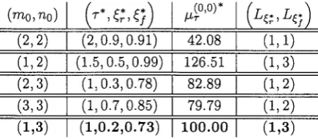
4.1 Optimal system parameters and inspection frequencies for different

(mo, no)

86

4.2 An illustration of decision process and action process subject to the failure state process given optimal system parameters (T*,~;,~j)

= (1,0.2,0.73)

87 4.3 An illustration of decision process subject to the estimated. damage state

process /-l~ given the optimal decision thresholds . . . .. 87 5.1 An eVolution of optimal expected revenue V*, mean inspection times fl

and mean time between inspections .6.fl given the optimal control process u* and linear transition rate . . . 131 5.2 An evolution of optimal expected revenue V*, mean inspection times fl

and mean time between inspections .6.fl given the optimal control process u* and nonlinear transition rate . . . 139

1.1 An evolution of the preventive replacement . . . .. 12

1.2 An evolution of the system state given Wiener process (65) and maximum

process (56) . . . 14

1.3 An evolution of the system state given Gamma process (74) 15

2.1 Ten observations from the malignant melanoma study, calendar time (years) 18

2.2 Ten observations from the malignant melanoma study, years since opera-_{. I . ,}

t~on ( survival time). . , . . . 18

2.3 An evolution of the counting process Nt 25

2.4 A realization of a 3-variate counting process 27

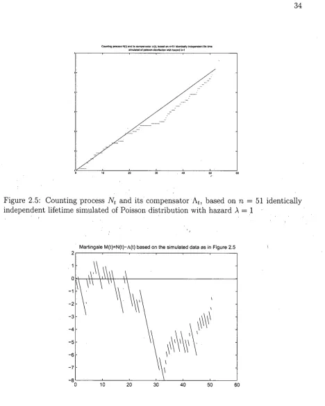
2.5 Counting process Nt and its compensator At, based on n

=

51 identically independent lifetime simulated of Poisson distribution with hazard A

=

1 34 2.6 Martingale _{M t}

=

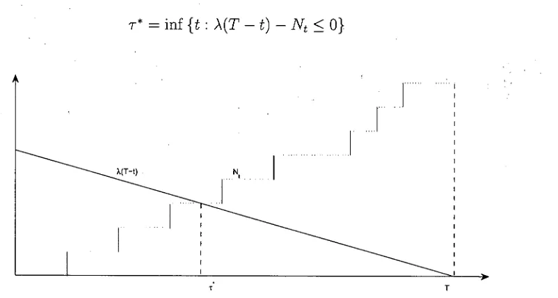
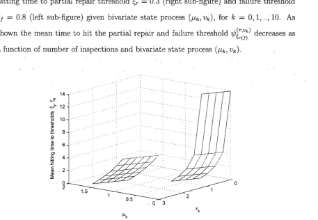
Nt - At based on the simulated data. 35 2.7 The Optimal Stopping Time T* . . . 37

4.1 Mean hitting time to partial repair and failure threshold ~r

=

0.3, ~f

=

0.8 as a function of bivariate state process (f.-Lk, Vk), given T

=

0.32, ~

=

0.8

and (m, n)

=

(5,11). . . . . . . .. 83

4.2 An evolution of expected time to inspection given the start state (X_o, Va) =

(x, v), for 1jJ(x)

=

x,

AO(t)

=

t

and (3

=

1. . . .. 93 5.1 An evolution of the mean residual waiting times in the state one given

qf(t)

=

u.t

and control values

u

= 0.1,0.5,1. . . . 116

5.3 An evolution of the optimal expected revenue V(t, n), t E [0,15]' (0

:s;

n

:s;

12) . . . 129

5.4 An evolution of the inspection intensity

i(n,

t, u*) given the optimal con-trol process

u; . . .

131

5.5 An evolution of the mean time between inspections (MTBI) given the

optimal control process

u; . . .

132

5.6 An evolution of failure intensity ~(n, t, u*) given the optimal control

pro-cess

u; ... ' ...

133

5.7 An evolution of sojourn time distribution of the damage process Xt in

state one given control (repair degree) values u = 0.4,0.8,1 and

parame-ters a = -0.25, b = 1. . . . . . . . . 135 5.8 An evolution of probability of state one

<pU(O, t,

1) given control (repair

degree) values u = 0.4,0.8, 1. . . 137

5.9 An evolution of optimal expected revenue over finite time [0,4]. 138

5.10 An evolution of optimal control process u* given FN. . . . 140

5.11 An evolution of optimal inspection intensity

i(n,

t,

u*) given FN. 140 5.12 An evolution of optimal failure intensity ~(n, t, u*) given FN. . . . 142

6.1 An evolution of the deterministic flow of the process <Pt driven by the

control process Ut, the virtual age process

vt

= VTn

+t (0

:s;

t

<

Tn+l - Tn)

(0

:s;

n

:s;

2) corresponding to nth jump time Tn with the repair degree

~n(O

:s;

~n

:s;

1) and VTn+1 = VTn

+

~n¢(Tn+l - Tn) . . . 149

6.2 An evolution of the maintenance process subject to stochastic deterioration 150

General notation

Decision model

• ~r: partial repair threshold

,

•

~r failure threshold

• ~: degree of imperfect (partial) repair

• Tn: nth inspection time

• Tn: nth inter-arrival inspection time

• T: period bf inspection

• {3: repair alert parameter.

• AD: baseline intensity function

• AD: cumulative baseline intensity function

• A: failure intensity function • C: inspection cost of the system • C f: replacement cost of the system

• C~(v

+

T):

minimal repair cost of the system subject to periodic inspection policy • C~(v

+

~T): partial repair cost of the system subject to periodic inspection policy • C~(v

+

T(X,V;(3)):

minimal repair cost of the system subject to non-periodic

in-spection policy

• c~(v

+

~T(X, v;

(3)):

partial repair cost of the system subject to non-periodic in-spection policy

Intensity control model

• Pn+l: (n

+

1)th expected inspection time

• Vn: time between (n _1)th and nth inspection time

• q12(t):

transition rate from normal state

(X

t

=

1) to degraded state

(X

t

=

2) given

control process Ut

=

U

• 'Yi: inspection intensity of the system when the state of the damage process Xt is

i E S =

{1, 2}

• K: inspection cost of the system when operating in state two (Xt

= 2)

• K - C: inspection cost of the system when operating in state one (Xt

=

1)

• k€(t, u):

repair cost per unit time with repair degree U

• J-li: revenue per unit time when the state of the da.mage process is i E S

• (Pi:

replacement cost when the state of the damage process is i E

S

Stochastic processes

• Xt : physical state (damage) process reflecting the effect of operating environment

• Vt:

virtual age process

• N( stochastic process counting the number of inspections up to time t

• FtN: filtration generated by the counting process of inspections Ns up to time

t

• Xn:- physical state process just after nth repair

• Vn: virtual age process just after nth repair

• An:

filtration generated by the history of bivariate state process (Xk' V_k): k

=

1,2, ... ,n

• Ut: control process at time

t

representing the decision at time

t

to perform a repair

with repair degree U

• u;:

optimal control process at time t

• T*: optimal production run length of the manufaCturing system

• Td: first passage time of darriage process Xt from normal state to degraded state

• T(Xn' V_n; {3): inspection scheduling function (xn, V_n; {3) -+ T(Xn' V_n; {3) adapted to

partial information

An

measuring expected time between nth and (n

+

1)

th

inspec-tion given that the state of process just after nth repair is (Xn,

V

_n)

=

(xn' v_n)

• FU(t):

sojourn time distribution in state one (Xt = 1) given control process Ut = U

• Ft(Xt,Vt): failure distribution function given bivariate state process (Xt,

Vt)

• Ft(Xt,Vt): survival function given bivariate state process (Xt,

Vt)

• RiXn,vn): failure state process just after nth repair given bivariate state process

• RiXn,vn): conditional survival function just after nth repair given bivariate state

• fr(ylx):

transition probability density function of

Xr

=

y

given

Xo

=

x

• f.e(Ylx):

transition probability density function of

Xr(x,v;.B)

=

y

given

(Xo,

Va)

=

(x,v)

• TJx,v) :

hitting time of modified partial repair threshold

'l/Jtn,vn-

1

) by the process

~~"',1)) r

Xn

with periodic time to inspection T given that the process initially started from

state

(Xo,

Va)

=

(x, v)

• rSx,v) :

first hitting time of modified failure threshold

'l/Jtn,vn-

1

) by the process

Xn

'I-'~(.,.,v) f

f

with periodic time to inspection T given that the process initially started from

state

(Xo,

Va)

=

(x, v)

• TJx,V) :

_~~i3,v) hitting time of modified

parti'~l

repair threshold

'l/J~.e,v)

by the process

X

t

. r

with expected time to next inspection

T(X,

v;

/3)

given that the process initially started from state

(Xo,

Va) = (x, v)

•

T.~,x,v)

:

first hitting time of modified failure threshold 'l/J~.e,v) by the process

X

_t with

'I-'~(i3,v) . ~f·

f .

expected time to next inspection

T(X,

v;

/3)

given that the process initially started

1 from state

(Xo,

Va) = (x, v)

•

C~x,v):

cost of inspection and repair per cycle with period of inspection T given

that the process initially started from state

(Xo,

Va) = (x, v)

• J.Ldx,v): expected cost of inspection and repair per cycle with period of inspection

T given that the process initially started from state

(Xo,

Va) = (x, v)

•

L~x,v): length of a cycle with period of inspection T given that the process initially

started from state

(Xo, Vo)

=

(x,

v)

• J.L L~x,v): expected length of a cycle with period of inspection T given that the process

initially started from state

(Xo, Vo)

=

(x,

v)

• J.L~x,v): expected cost of maintenance per unit time with period of inspection T

•

c~x,v):

cost of inspection and repair per cycle with expected time to next inspection

T(X, v;

f3)

given that the process initially started from state

(Xo,

Va)

=

(x, v)

• f.Ldx,v): expected cost of inspection and repair per cycle with expected time to next

{3

inspection

T(X,

v;

f3)

given that the process initially started from state

(Xo,

Va)

=

(x,v)

•

L~x,v):

length of a cycle with expected time to next inspection

T(X,

v;

f3)

given that the process initially started from state

(Xo,

Va)

=

(x, v)

• f.LL(x,v): expected length of a cycle with expected time to next inspection

T(X,

v;

f3)

• {3

given that the process initially started from state

(Xo,

Va)

=

'(x, v)

• f.L~x,v): expected cost of maintenance per unit time with expected time to next

T(X,

v;

f3)

given that the process initially started from state

(Xo,

Va)

=

(x,

v)

• <j;U(n, t; i): probability- measure of state i E S of damage process X at time t E

"

[Pn, Pn+l)

given control process Ut= u

• i'(n, t; u):

inspection intensity at time

t

E

[Pn, Pn+l)

given control process Ut

=

U

• r,n+l:

inspection scheduling function adapted to partial information FN measuring expected time between nth and (n

+

1)th inspection

•

~(n,

t;

u): failure rate of the system at time

t

E

[Pn, Pn+d

given control process

During the past decades to prevent catastrophic failure of the system, avoiding poten-tial costs arising from the system downtime and optimize maintenance costs, there has been an interest in maintenance optimization problem for repairable systems subject to deterioration.

Here to tackle the maintenance optimization problem two maintenance models for deteriorating repairable systems are proposed: optimal preventive maintenance schedul-ing model tdecision model) and optimal maintenance-r~pa~r and inspection-scheduling model (intensity control model). In chapter 4 under both periodic and non-periodic in-spection policy a novel approach to the determination of optimal repair and replacement decision rule subject to system parameters is presented. A renewal argument is used to derive expressions for the long-run average cost per unit time under theses two kinds· of inspection policy. The second part of the research (see chapter 5) considers mainte-nance scheduling problem of manufacturing systems whose production process (resulting output) is subject to system state. The latter means, resulting outputs (revenue) from system depends on the deterioration level of the manufacturing system: the good state of the system results in more efficiency of the system and more resulting output (rev-enue); the bad state of the system leads to system malfunction and less revenue. To optimize revenue from the manufacturing system, using optimal intensity control model, an optimum repair and inspection policy to balance the the amount of maintenance re-quires to increase system efficiency against the loss of revenue arising from the system malfunction is presented. Our approach rests on assumption that the transition rate from good (normal) state to bad (degraded) state is linear/non-linear.

After five years, in spite of some difficulties, fortunately my thesis is in a position to be submitted. Definitely, if I was financially supported more, the quality of my thesis would be better.

I would like to thank Prof. Martin Newby, my supervisor, for his many suggestions during this research and introducing this applied and interesting research topic. I am also thankful to Prof. Andrew Jardine who provided many useful references. I had the pleasure of meeting Prof. Nozer D. Singpurwalla at the MMR 2009 Conference. I wish to thank him for his constructive comments. He is a wonderful person.

I

am also grateful to Prof. Kel1 Grattan, Prof. Nicos Karcanias and Prof. Martin Newby for providing me with financial support, the ORS Scholarship, which was awarded to me for the period 2006-2010, and 10 months Bursary which were crucial to the successful completion of this research. I would like to thank Dr. Halikias and Dr. Gerrard who have given me opportunity for getting some teaching experience in City university.

Of course, I am grateful to my parents for their patience and love. Without them this work would never have come into existence.

Finally, I wish to thank the following: Prof. Majid Asadi, my B.Sc and M.Sc supervisor in Isfahan university who introduced me to reliability area; my sister, Sanaz; my brother, Mahmood and my brother in law, Alireza J annesary.

Problem Statement

In this chapter two maintenance optimization problems which are of great practical importance are considered: optimal preventive maintenance scheduling problem for a stochastically deteriorating system (Decision model) and optimal maintenance schedul-ing problem for a manufacturschedul-ing system subject to'deterioration (intensity control model).' In both decision and intensity control model to optimize maintenance pro-cess we provide a solution to the optimal control of amount of maintenance in such a way that the maximum revenue from manufacturing system and minimum maintenance cost are derived respectively. In the first model (see chapter 5) which is a novel approach to the maintenance modeling, using intensity control model, the optimum revenue from manufacturing system is achieved by an optimal control (repair degree) process keeping a correct balance between revenue from system and amount of maintenance. In the second model (see chapter 4), using traditional method (embedded renewal process), we find an optimal solution the repair decision thresholds and system parameters. The optimal decision thresholds and system parameters as optimal (repair degree) control process provide a right balance between amount of maintenance and maintenance cost.

1.1

Maintenance scheduling problem of systems

sub-ject to non-self announced failure

Failure of many systems such as protective devices or stored items that are subject to random failure is not self-announced and can be found only by inspections which incur costs in terms of wage and material. It .stands to clear the ,greater the probability of detection of failure, the higher the inspection costs. So, to minimize the cost keeping a correct balance between frequency of inspections and inspection costs is essential. The literature on the opti.mal inspection problem for systems subject to non-self announced failure is vast. Barlow et al (7) given some major assumptions which include the system failure is non-self announced and inspections do not impact on the failure characteris-tics, shows that optimal inspection times are the solution of system of equations. He

l .

number. Both conditional failure probability based models are known as one-parameter optimization models. As mentioned before, at survey times inspections due to either certain recovery actions (e.g. some adjustment, or partial repairs) or the system com-plexity do not impact on the failure characteristics of the system. That means, the system state at inspection times leaves unchanged. Such inspection problem which is most common in application is addressed by Jiang and Jardine (32). They present an optimum inspection schedule subject to an increasing failure rate. It is assumed that failures occur at random times and can be detected only through an inspection. Major problems of inspection models are that those either are restricted to some assumption, computationally complicated or in view point of optimal inspection times do not provide good accuracy. In summery the algorithms introduced above do not create an accurate solution for the inspection time sequence to the optimal inspection problem. Irrespective of the BHP model which "is extremely sensitive to time

t

1 , it· seems this problem arises

from some subjective parameters.

The basic system of equations which is a basis to determine the optimal inspection sequence was first developed by Barlow et al (7). Barlow under a set of assumptions presents an optimal inspection model for systems which are subject to non-self an-nounced failure. That means, failures event is rand'om and can be detected only through an inspection. Based on Barlow maintenance model, inspections do not affect on the failure characteristics, inspection ceases upon detection of failure and at inspection times no repair takes place.

The system of equations associated with Barlow cost model that is

is given by

or, equivalently,

8C =0

8t, ₁

0' _ F(t j ) - F(tj-l) _ Cl

1 - f(t_{j )} C2

(1.1.2)

Vj

=

1,2, ... (1.1.3) where F(t) is failure distribution function, {tj= 1,2, ... }(to = 0) and OJ = tj+l - tj

denote the inspection time sequence and inspection interval sequence respectively and

Cl, C2 refer to the cost per inspection and the cost per unit time of a system being

un-available due to an undetected failure, respectively.

Barlow to find a solution for the system of equations (1.1.3), which is a sequence of

op-timal inspection time, propose an algorithm widely called Barlow, Hunter 'and Proschan

algorithm(BHP algorithm). The BHP algorithm is computationally cumbersome and

has restrictive assumptions, being extremely sensitive to the vaJue of

h,

the 0rsequence

generated from equation (1.1.3) is the major problem of BHP algorithm. In preference

to the Barlow model and a few nearly optimal algorithm, some often methods which fall

into the categories outlined below are presented:

• Improvement of the original algorithm (see Nakagawa and Yasui (50));

• Approximate methods associated with the concept of an inspection density function

(see Keller, Kaio and Osaki (34));

• One-parameter optimization models. This category contains an assumption on the

failure model. For example, Munford and Shahani (48) assume that the conditional

failure probability is constant. Chelbi, Ait-Kadi (11) suppose that the conditional

1.1.1

Improved method of the original algorithm

The method presented by Nakagawa and Yasui (50) is associated with the parameter

c E (0,

cd

C2) and a sufficiently large

tn

such that

or, equivalently,

(1.1.4)

So, with respect to known values that are C1, C2,

tn

and c, the equation (1.1.~) gives

the

(n -

l)th inspection time tn -1 and the rest of inspection times tj, j

<

n -

I, can be

(I recursively evaluat~d from the equation (1.1.3). According to the Nakagawa and Yasui model (50), the process carries on ~ntillh(e.g. j=n-K) step where

F(t

n -K - 1 )

<

0 or

tn-K

>

2tn-K -1' :Two problems associated with this algorithm are the resulting sequence

of inspection times is sensitive to the parameter c and the value

tn.

Besides, if the value

of t1 resulting from above algorithm is applied in equation (1.1.3), the BHP algorithm

produces a totally different solution. This deficiency arises from the fact that their

algorithm introduces an inappropriate condition

F(t

n -K - 1 )

<

0 to replace the condition

to

=

F(to)

=

O.

1.1.2

Approximate method associated with an inspection

den-sity function

Keller (34) with assumption that the time between the failure and its detection is half

presents the inspection density concept

n(t)

which denotes the number of checks per unit of time. Where

t

is the failure instant if the failure occurs within

(tj,

tj+l)'

According to the Keller model the inspection time sequence in terms of

n(t)

is obtained as

to

=

0,

tj

=

tj-l

+

1jn(t

j _ 1

),j

=

1,2, ... (1.1.5)

where

n(t)

=

2;1(~~2 and

r(t)

denotes the failure rate function.

Kaio and Osaki (34) show that the inspection time sequence resulting from the equa-tion (1.1.5) is not accurate. This problem comes from dependency of

tj

to the inspection intensity

n(t)

evaluated at the left ending point of the inspection interval

(t

j - 1 ,

t j).

To

resolve the problem following equation to evaluate the inspection time sequence is sug-gested:

"

l

tj

n(t)dt

~

1, j

=

1,2, ...

t j - l

(1.1.6) The problem of above method is rack of improvement in accuracy of evaluation of inspec-tion sequence. Moreover, it is computainspec-tionally more complicated than BHP algorithm in the case that the failure distribution is not Wei bull.

1.1.3

One-parameter optimization method

The conditional measure

Pj

=

1-

R(tj)j R(tj-

1 ) which is the probability that the system

fails over time interval (tj -1 ,

tj)

given that it survives beyond time tj -1 is considered

as a basis to evaluate the inspection time sequence. By assuming above conditional probability is constant p, Munford and Shahani (48) define a sequence of inspection times.

number of inspections (or, failure rate). More precisely,

l / j . 1 2

Pj

=

Pl , J

= , , ...

(1.1. 7)

In both methods which define an one-parameter optimization model the parameters P and Pj are determined such that the minimum expected total cost given by (1.1.1) is achieved.

1.2

Maintenance scheduling problem

of systems

sub-ject to self announced failure

Locket (45) to relate machine type to system failure rate defines a constant" k" which can be found from experience. As noted in all of the above cited models, the system failure rate over its entire life has a largely constant. But, in the deteriorating state it is expected the system has a steadily increasing failure rate. Hence, an optimal model for frequency of inspection needs to be time dependent. This ensures that the frequency of inspection can respond to variation in the failure rate over time. To meet this defi-ciency the time dependent inspection factor

(IF)

is introduced as a key tool to reflect variations on the fai.lure rate (Jardine (29); Dhillon (23); Kececioglu (36); Locket (45); Wild (76)). It is assumed that the failure rate is inversely related to the time dependent inspection factor. This realistic assumption ensures that as inspection is performed and the frequency of inspection increases, the failure rate decreases. Several variations in-cluding the inverse law (Jardine (29); Dhillon (23); Kececioglu (36); Locket (45); Wild (76)), negative exponential, increasing influence of hazard rate and decreasing influence of hazard rate (Mathew (47)) in defining IF have been examined.

problem of manufacturing systems whose resulting output (production process) is sub-ject to deterioration is vast. The earlier works on preventive maintenance models with production processes with more than one operating state and a failure state are given by Derman ((21),(22)), who studies a process that deteriorates moving through a finite number of states according to a Markov chain. Derman assumes that the state of the process is known with accuracy at all discrete points in time and show that the optimal replacement policy is a control limit policy; that is, the equipment should be replaced as soon as it is observed to operate in a state worse than some critical state. The same result is also obtained by Kolesar (39) for a similar model but with a more general cost function. The process operating states can alternatively be expressed by the magnitude of the cumulative damage or wear of equipment. The process is asspmed to be subject to exterior shocks that damages or causes wear to the equipment, thereby increasing its probability of f~ilure. Shock models have been introduced by Taylor (72) and they have been studied by Feldman (25), Bergman (8) and Valez-Flores and Feldmanv

effect of PM activities on the deterioration pattern of the process. The model is based

on assumption that after PM, the aging of the system is reduced proportional to the PM

level and the state of the production process is improved by minimal repair or stopped

followed by the restoration work depending on it is in a type I out-of-control-state or

in a type II out-of-control state. Using examples of Weibull shock models, Sheu shows

that performing PM will yield reduction in the expected total cost. Wang and Pham

(75) present a general repair model to maintenance optimization of production systems

subject to deterioration. The effect of deterioration is reflected in higher production

costs and lower product quality. To keep production costs down while maintaining good

quality, Wang and Pham (75) suggest an optimal periodic maintenance 'model in which

both preventive and corrective maintenance are imperfect.

Apart from' the maintenance literature, deterioration of the process condition is also

a standard feature of the' statistical process control model in the quality field. The

process is assumed to operate in the" good" quality state (in-control) until it shifts to

an inferior quality state (out-of- control) as a consequence of the occurrence of some

assignable causes. The time until transition to an out-of-control state (quality shift) is

usually assumed to be exponentially distributed (Poisson process) but other

distribu-tions have been considered as well (Banerjee and Rahim (6)). In a model of a process

with non-exponential transition times Rahim and Banerjee (64) introduce the use of the

preventive maintenance actions to ptotect the equipment against quality shift. In

par-ticular, Tagaras (71) uses a Markovian approach similar to that of Derman ((21),(22)) to

describe the evolution of production processes characterized by several quality states (a

single in-control state and multiple out-of-control states) and a single failure state. He

simultaneously considers quality control and quality control parameters that minimize

In preference to above maintenance models, here we present a novel approach to main-tenance scheduling problem of a manufacturing system subject self-announced failure. The model is superior to existing maintenance scheduling models based on inspection strategy. The approach rests on assumptions that the resulting output (revenue) from system is subject to the system state influenced by repair action and deterioration pro-cess. Insufficient maintenance leads to an increase in the number of detective items, low profit and low maintenance cost; excessive maintenance results reduces the proportion of defective items, high profit and high maintenance cost. In chapter 5 to tackle above maintenance problem, using optimal intensity control (10), an optimal solution to the determination of the amount of maintenance i.e., frequency of inspection and repair de-gree of the system is obtained. In contrast to former maintenance models, the intensity

. . ' .

control based mode~ presented in chapter 5 not only does not suffer from sorrie subjectiv:e concepts, but also gives an insight into various measures such as prediction of system failure, conditional mean time to failure of the system and optimal inspection intensity and also optimal production run length of the system. Besides, it has the potential to be extended to tackle technical maintenance problems which are common in application (see chapter 6).

maker must than take action to restore the situation.

1.3

Preventive maintenance scheduling problem

Decision modeling for deteriorating systems which is of great practical importance in industry have been widely studied in literatures. Jardine (31) under periodic inspection policy introduces a condition based maintenance (CBM) model subject to cost. The monitoring information to detect the condition of item is incorporated into proportional hazard model (PHM) (13) through underlying Markov stochastic process

Z(t).

Deci-sion making is given both the age and condition of components at inspection times. The basic decision nile which is used immediately after inspection instant is to replace the system if the item fails or deterioration level. of the item (ri$k) described by the (PHM)

(h(t, Z(t))(t

2:

0) exceeds a threshold level (prev'ent,ive replacement); otherwise operation can continue (see Figure 1.1) (30). He sh~wed that the optimal replacement

risk

h

-time

h(t,Z(t)) . hazard function

h -

hazard level

6 . inspection interval

tR -

preventive replacement

Figure 1.1: An evolution of the preventive replacement

[image:28.575.67.497.314.617.2]

replacement is performed either at failure or when failure rate of the system reaches or exceeds an optimal failure threshold g*:

T* = min {T, inf {t ~ 0 : h(t, Z(t)) ~ g*}}.

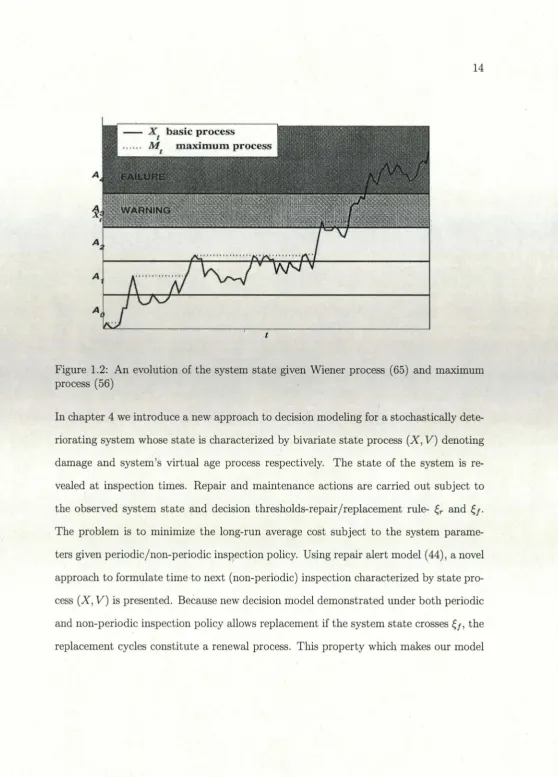
Where T and T* denote the failure time and optimal replacement time of the system. Newby and Dagg (56) study an optimal inspection policy for a deteriorating system whose evolution is described by a stochastic process. The inspections and repair actions to avoid catastrophic failure of the system are with respect to warning limits (threshold) which classify the state space into some non-overlapping regions. At inspection times the decision maker subject to the system state has disposition to leave the system to continue to operate or replace it by new one (perfect repair). The cost is considered as a criterion to determine an optimal inspection policy. The model represented by (56) is appropriate for crack growth models (see (53), (54), (70), (12)) which is a basis for some physical phenomenons such as fatigue crack growth problems, offshore structure, and coastal flood barriers subject to erosion (57). Roughly speaking this suitability comes from the fact that the system is regarded as failed if the system state crosses the failure threshold (see Figures 1.2, 1.3).

- X basic process

t M

t

A

A

A

t

Figure 1.2: An evolution of the system state given Wiener process (65) and maximum

process (56)

In chapter 4 we introduce a new approach to decision modeling for a stochastically

dete-riorating system whose state is characterized by bivariate state process (X, V) denoting

damage and system's virtual age process respectively. The state of the system is

re-vealed at inspection times. Repair and maintenance actions are carried out subject to

the observed system state and decision thresholds-repair/replacement rule- ~r and ~f'

The problem is to minimize the long-run average cost subject to the system

parame-ters given periodic/non-periodic inspection policy. Using repair alert model (44), a novel

approach to formulate time-to next (non-periodic) inspection characterized by state

pro-cess (X, V) is presented. Because new decision model demonstrated under both periodic

and non-periodic inspection policy allows replacement if the system state crosses ~f' the

[image:30.575.9.568.24.802.2]

Figure 1.3: An evolution of the system state given Gamma process (74)

distinguished to the models (55) and (56) is used to derive expressions for the long-run

[image:31.575.12.569.41.774.2]

Some Fundamental Concepts

2.1

Introduction

, '

To set up the repair and maintenance models which are preventive maintenance schedul-_, ing model for deteriorating systems (see Chapter 4) and maintenance scheduling model for a manufacturing system subject to deterioration (see Chapter 5) providing some mathematical tools is required. Following section is devoted to presenting an informal definition of some stochastic notions including intensity process, filtration, and martin-gale which are the solid basis in stochastic processes theory. The next section is oriented to give a formal definition of history of the process remarked by filtration

F,

stochastic process and F-adapted process. Section 4 and 5 give a detailed discussion of univariate, multivariate point process and measurability with respect to filtration

F.

To provide fundamental requirements of the research, section 6 and 7 are assigned to give some mathematical techniques which are stopping time and martingale theory. Also, in sub-sequent section a formal definition of stochastic intensity with respect to filtration F

is given. Finally, to model the failure of the system influenced by some variables such

as environmental factors and system's age and repair and maintenance process ,which state history of the process, some intensity process models are represented.

2.2

An introduction to the basic concepts

Let Xl, X2 , ... ,Xn be n (n

2::

1) (uncensored) continuously distributed survival times

from a survival function

S

with hazard rate function a; thus, a

=

1/(1 -

F)

where F

= 1-

Sis the distribution function'and

1

the density of the Xi for i

= 1,2, ... ,

n. The hazard rate a completely determines the distribution through the relation

(2.2.1)

One can inte'rpret a by the heuristic

P(Xi

E

[t, t

+

dtllXi 2::t)

=

atdt.

(2.2.2) Typically, in survival analysis problem, complete observation of Xl, X2 , ... , Xn is not

possible. Rather, one only observes

_{(Xi, Di),}

where

Di

is a "censoring indicator," a zero-one valued random variable describing whether Xi or only a lower bound to Xi is observed; namely,

(2.2.3)

We shall consider

Xl, X

2 , ... ,

Xn

as random times; at these times, the value of the

cor-responding

Di

becomes available, and we know whether the corresponding event is a failure or a censoring. Thus, all n survival periods start together at time

t

=

O.

10,---~---.---._----_.---._----_,----_.

8

6

4

2

OL-____ - L _ _ _ _ _ _ L -_ _ _ _ - L _ _ _ _ _ _ ~ _ _ _ _ ~ _ _ _ _ _ _ ~ _ _ _ _ ~

. 1964 1966 1968 1970 1972 .1974 1Q76 1978

Figure 2.1: Ten observations from the malignant melanoma study, calendar time (years)

12r---.---.---r---.---.---10 r

-8

f---6 f---.

4 r---.---.-.. --.

2 ----.---.---.. ----.----... ----.---.-.--.--.---.----...

:

-O~---~---~---~---L---~---~

o

2 4 6 8 10 12

[image:34.575.63.516.58.655.2]

Years since operation

scale

t

years since operation. This latter time scale is the one we concentrate in our

illustration of stochastic process concepts. A line with the filled circle corresponds to

Di

=

1 (a failure), a simple line to Di

=

0 (a censoring).

Further analysis is difficult without an assumption of right censoring. we will make

the most general assumption which still allows progress: the assumption of independent

censoring, which means that at any time

t

(in the survival time scale) the survival

ex-perience in the future is not statistically altered (from what it would have been without

censoring) by censoring and survival experience in the past. To formulate this notion, we

must be able to talk mathematically about past and future. This will be done through

the concept of a filtration or history (F_t)t2:o; F_{t representing the available data at time}

t.

We write Ft - corresponding for the available data just before time

t.

A specification

of (F_{t)t2:o can only be done relative some observer, and different observers may collect}

more or less information. But for all observers, as time proceeds, more information

become available.

The notion of a filtration is defined as an increasing family of O'-algebras defined on the

sample space. In our simple example, we will simply take Ft to mean the values of

Xi

and Di for all i such that

Xi ::;

t,

otherwise just the information that

Xi

>

t.

For Ft

-the obvious changes must be made: ::; becomes

<

and the> becomes ~.

The independent censoring assumption can now be written (still very informally) as

(2.2.4)

Compare this to (2.2.2). Replacing the probability on the left-hand side by the

E

(#

{i :

Xi

E

[t, t

+

dt), Di

= 1 } IFt- ) =

#

{i :

Xi

2:

t} atdt

=

Yt,at dt

= At

dt ,

which we have defined the processes Y and A by

(2.2.5)

the number at risk just before time

t

for failing in the time interval

[t, t

+

dt),

or the size of the risk set, and

where

#

is a counting notation.

Now formula (2.2.5) can be interpreted as a martingale property involving a certain counting process (3); in this case, the process

N

=

(Nt)t?o

counting the observed failures

Nt

=

# {

i :

Xi

~

t, Di

= 1 }

and its intensity process

A.

Let us write

_dNt

or

N(dt)

for the increment

_{NHdt- -}

Nt-of

N

over the small time interval

[t, t

+

dt).

Therefore, we can rewrite

(2.2.5)

as

(2.2.6)

Note that the intensity process is random, through dependence on the conditioning ran-dom variable Ft -.

To explain the meaning of the martingale property, first define the integrated or cumu-lative intensity process A by

and the compensated counting process or counting process martingale M by

Or, equivalently,

(2.2.7)

Consider the conditional expectation, given the strict past Ft -, of the increment (or

difference) of the process

M

over the small time interval

[t, t

+

dt);

by (2.2.7), we find

E(dMtIFt-)

=

E(dNt - dAtIFt-)

=

E(dNt - AtdtIFt-)

(2.2.8) ~

_{E(dNtIFt-) - Atdt}

= 0,

. where the last step is precisely the equality (2.2.6), noting that

At

is measurable with

. \ respect to the filtration Ft -. Now, relation (2.2.8) says that A is the compensator of N,

or that M = N - A is a martingale for all

t.

In wide generality, we have that any counting process N, that is, a process taking the

values 0,1,2, ... in turn and registering by a jump from the value (k - 1) to k the time

of the kth occurrence of a certain type of event, has an intensity process A defined by

Atdt

=

E(dNtIFt-).

The intensity process is characterized by the fact that

M

=

N -

A, where A is the corresponding cumulative intensity process, is a martingale remarked

by a fair game (see section 2.7). The martingale property says that the conditional

expectation of increments of M over small time intervals, given the past at the beginning

of the interval, is zero. This is (heuristically at least) equivalent to the more familiar

definition of a martingale

(2.2.9)

dt)

=

(5,

t],

we find

=

1

E (E(dMul.1'u-I.1's))

s<u:::;t

(2.2.10)

= 0.

Version (2.2.9) of the martingale property is much easier to make the basis of a mathe-matical theory.

2.3

Filtration

We are going to model the occurrence in 'time of random events;in fact, discr;ete events occurring in continuous time. So we fix a continuous time interval

'r/

=

[0,

T) or

[0,

T]

For a given terminal time T,

°

<

T ~ 00. Note that the terminal time point T mayor

I

may not be included; this varies from application to application. We write fj

=

[0,

T],

the time interval augmented with its endpoint if it was not first present.

Definition 2.3.1. (Filtration) (3) Let (D,

.1', P)

be a probability space. A filtration

Also called a history, is an increasing right continuous family of sub-O'-algebras of

.1'.

In the standard theory we use, it is often assumed also to be complete in the strong sense that, for every

t,

the O'-algebra

.1'

t contains all P- null sets of

.1'.

However, the

results of the standard theory.

When the complete set of assumptions hold, we say that (Ft ) satisfies the usual

condi-tions:

F8

~

F

t ~

F

for all s

<

t (increasing)

F8

=

n

F

t for all s (right continuous) t>8

A

c

B

E

F, P(B)

=

0 =?

A

E

Fo

(complete)

(2.3.1)

The O"-algebra Ft is interpreted as follows: It contains all events (up to null sets) whose

occurrence or not is fixed by time

t.

There is also a pre-t O"-algebra containing all F8 ,

s

< t;

it contains events fixed strictly before

t .

. " It is most common the filtration to be described as the history generated by a

stochas-tic process. X. This means that Ft is the O"-algebra generated by X8 , s ::;

t.

Definition 2.3.2. (Stochastic process) (5) A collection of random variables X

=

Xt ,

t

~

o

defined on the same probability space

(Sl, F,

P) is called a stochastic process.

For any fixed

w

E

Sl

the real function

X (., w)

is called the path of a stochastic process

X.

Definition 2.3.3. (F-adapted) (5) A stochastic process is adapted to the filtration F

if for any fixed

t

~ 0 the random variable Xt is Ft measurable, i.e. for any Borel set B

of IR the event

{Xt

E

B} EFt.

2.4

Point Processes

Definition 2.4.1. (Univariate counting Processes) (10) A realization of a point process

over [0, (Xl) can be described by a sequence Tn in [0, (Xl) such that

This realization is, by definition, nonexplosive iff

Too

=

lim Tn

=

00. n ... oo

To each realization Tn corresponds a counting function Nt defined by

Nt

= {

n

+00

if

t

E

[Tn, Tn

+1) , n ~ 0;

if

t

~ Too.

(2.4.1)

Nt is therefore a right-continuous step function such that No

=

0, and its jumps are upward jumps of magnitude 1 (see Figure 2.3). In addition, if E[Ntl is finite for all

t

then the point process is said to be integrable.

N,

;

T, T,

Figure 2.3: An evolution of the counting process Nt T,

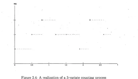
Definition 2.4.2. (Multivariate Counting processes) (10) Let Tn be a point process

defined on (D, F, P), and let

(Zn'

n ~ 1) be a sequence of 1,2,3, ... , k-valued random

variables, also defined on (D, F, P). Define for all i, 1 ::; i ::; k, and all

t

~ 0:

Nt(i)

=

L

1

(Tn ::; t)J(Zn

=

i).

(2.4.2)

[image:40.574.57.513.47.574.2]

Both the k-vector process Nt

=

(Nt(1), ... Nt(k)) and the double sequence (Tn, Zn, n ~ 1) are called k-variate counting processes.

As noted the Nt

(i)'

s have no common jumps. In general we say that two point pro-cesses N t(1) and N t (2) defined on (0, F, P) have no common jumps

if 6.

Nt (1)6.Nt(2)

=

0,

t

~ O,P-a.s.

Following examples show application of both univariate and multivariate point process to the renewal process and Markov renewal process modeling.

Example 2.4.1. (Renewal Process) Let {Tn}, n

= 0, I, 2, ...

denote a sequence of

non-negative random variables defined on (0, F) and To

=

O. We introduce Xi

= Ti -

~-1'

i = 1, 2, ... as ith independent inter-arrival times distributed identically with finite mean value E(X)

<

00. It means after each renewal the process r~starts. It is easy to see :that

the counting process Nt:

I

Nt ;= I:~=11(Tn ::; t)

as a univariate point process or renewal process counts the number of renewals in

[0,

t].

Example 2.4.2. (Markov Renewal Process) Let J_{o denote the initial state of a repair}

process; and for n ~ 1, let In be a Markov chain with transition probabilities Pij denoting

the repair state of the process following nth repair and maintenance action (transition).

So, the process I_{n, n}

= 1,2, ...

that can be called as the External Process is a Markov chain controlled by the transition probabilities Pij'

Now, let Ni(t) refer to the number of repair times at which post repair states that are at

disposition of a controller are i (i

= 1,2, ... ,

k) value over time interval (0, t]. Now, if

Z(t)

=

IN(t)

can be treated as the repair state of the process at time

t

and the set

named a Markov Renewal Process can be treated as a k-variate counting process.

The Figure 2.4 shows an evolution of the multivariate counting process given k = 3.

N(t)

o ..

+ .... + ... + .... . + ... .

I L -_ _ _ _ _ _ ~ _ _ _ _ _ _ - L _ _ _ _ _ _ ~ _ _ _ _ _ _ _ _ L _ _ _ _ _ _ _ ~ _ _ _ _ _ _ _ _

o 0.5 1.5 2.5

Figure 2.4: A realization of a 3-variate counting process

2.5

Measurability with respect to Filtration

F

Definition 2.5.1. (F-Progressive) (4) A stochastic process X is F-progressive or pro-gressively measurable, if for every

t

the mapping

(s,w)

--t

Xs(w)

on [0,

t]

x

n

is

[image:42.575.72.520.295.551.2]

B([O, t]) is the Borel O"-algebra on [O,t].

Obviously, every left-or right continuous adapted process is progressively measurable.

A more measurability restriction over the stochastic processes leads to the subsequent

definition.

Definition 2.5.2. (F-Predictable) (4) Let F be a filtration on the basic probability

space and let P(F) be the O"-algebra on

(0,00)

x

n

generated by the system of sets

(8, t]

x

A,

a

:s;

8

<

t,

A

E

Fs,

t >

o.

P(F) is called the F-predictable O"-algebra on

(0,00)

x

n.

A stochastic process X = (Xt )

is called F-predictable, if

Xo

is Fa-measurable and the mapping

(t, w)

--t

Xt(w)

on

(0, (0) x

n

into R is m~asurable with respect to P(F).

To get an impression on predictability of a stochastic process with respect to

filtra-.

.

tion, let

Then, it is said to be stochastic process Xt an F-predictable process if it is measurable

from information available just before time

t

i.e. Ft -. In other words,

Some further important terms on predictability of stochastic process are as follows:

• if the stochastic process Xt is predictable then it is measurable with respect to the

O"-algebra on [0,(0) x

n

generated by adapted left-continuous processes

• The value of a predictable process is known at the moment t if the history in the time interval [0,

t)

is known .

• Every left-continuous process adapted to F is F-predictable.

2.6

Stopping Time

Before giving a formal definition of Stopping time, let have following example concerning the risk theory. Suppose the

F

t adapted net profit rate

R

=

(R

t ), t E 1R+, which is

non-increasing in time, denotes the difference between the flow of the income resulting from a deteriorating system and the total maintenance costs up to time t. The question is when to stop processing the system (optimal operating time) so that a correct balance between rewards fforn system and the increasing maintenance costs due to repair and maintenance actions which results in the maximum revenue is derived. A reasonable candidate for optimal operating time of the system is

T = inf

{t : R

_{t :::;}

O}

which is the first time the risk process

Rt

falls below zero. The time T which in risk theory

is known the time to ruin and characterized by the information level Ft is informally

called IF-stopping time. Obviously, this time point at which the stochastic process R =

(Rt ) hits the certain level (0) is random, because its occurrence depends on evolution of

the process. Formally, such random times which are based on the information level not anticipating the future are defined as follows.

Definition 2.6.1. (Stopping Time) (4) Suppose IF =

(Ft ),

t E 1R+, is a filtration on the measurable space (D, F). A random variable T : D ~

[0,00]

is said to be a stopping

{T::;

t}

=

{W: T(W) ::;

t}

EFt

2.7

Martingale Theory

In addition to the predictable processes explained above, the other kind of stochastic processes known as Martingales (4) or a pure noise part of a stochastic process plays a fundamental and complementary role in the general theory of stochastic processes. In subsequent section under Doob Meyer Decomposition Theorem (see Bagdonavicious (5)) we see how martingales are constructed through subtracting an increasing process

At

from a stochastic process Xt known as the sub-martingale. Roughly speaking, if Xt is a

stochastic process then it can be decomposed as the sum of a drift or regression part

At

I

and an additive fluctuation described by a martingale M(

Also, in a slightly weakened version of Doob Meyer decomposition called Smooth Semi-Martingale (SSM) (see Jensen (4)), this notion is considered as unpredictable noise term with zero-mean value resulting from the subtraction of a stochastic process, and a smoothly increasing process.

Definition 2.7.1. (Martingale) (4) An integrable IF-adapted process X

=

(X_{t ),}

t

E lR+, is called a martingale if

and a sub-martingale is defined with above equality being replaced by

With taking expectation of both sides of the (in)equality it is followed

E(X

t )

=

(2':

,~)E(Xs) which state

• A martingale is 'constant' on average, and models a fair game

• Sub-martingale (Super-martingale) is increasing (decreasing) on average.

• X is a sub-martingale (super-martingale) if (-X) is a super-martingale (sub-martingale) .

Example 2.7.1. Let X be an integrable F -adapted process. Suppose that the increments

Xt , - Xs are independent of Fs for all

t

>

s, s,

t

E lR+. If Xo = 0 and the 'increments

Xt - Xs follow a poisson distribution with mean t :..- s for t

>

s, then X is a Poisson

process. Now X is a sub-martingale (or, increasing on average) because of

On the other hand we have

that means

(X

t -

t)

is a martingale Mt :

As seen the martingale term Xt -

t

is subtraction of a sub-martingale i.e. Xt and an

Theorem 2.7.2. (Doob-Meyer Decomposition) (5) Let X be a right continuous

non-negative IF sub-martingale. Then there exists a right continuous martingale M and an

non-decreasing right continuous predictable process A such that

E(At)

<

00 and

for any

t

~

o.

If

A(O)

=

0

a.s. then this decomposition is a.s. umque, z.e. if Xt

=

Mt

+

A;

for any

t

~

0

with

A*(O)

=

0,

then for any t ~

0,

The process A is called the compensator of the submartingale X.

Following a slightly weakened version of the Do.ob Meyer Decomposition T~eorem

termed as S.mooth semi-martingale (SSM) representation is introduced. SSM

representa-tion which plays

a:

key role to set up the maintenance models (see Chapter 4,5), allow the

process to be decomposed into a drift part and an additive random fluctuation described

by a martingale.

Definition 2.7.2. (Smooth Semi-Martingale) (4)

A stochastic process

Z

=

(Zt), t

E lR+, is called a smooth semi-martingale (SSM) if it

has a decomposition of the form

where

f

= (ft),t E lR+, is a progressively measurable stochastic process with

E

it

I

fs

I

ds

<

00 Vt E lR+

and

E

IZol

<

00 and

M

=

(Mt)

E

Mo

where

Mo

denotes the class of cadlag 1

martin-gales with

Mo

=

o.

Short notation:

Z

=

(f,

M).

So, because the martingale term is a mathematical model of a fair game with con-stant expectation function E(Mt) = E(Mo) = 0, the stochastic process Zt, t E lR+ can be considered as a diffusion, which varies randomly around the regression term with expected value zero.

Theorem 2.7.3. (Smooth Semi-Martingale)

(4)

Let Z

=

(Zt), t E lR+, be a stochastic

process on the probability space

(0,

F, P), adapted to the filtration F. If G1 , G2 and ~

C3 hold true, then Z is an SSM with representation Z = (f, M), where f is the limit

defined in G1 and 1111 is an IF -martingale given by

And G1 , G2 , and G3 with assumption of

are

C1 . For all t, h E lR+ versions of the conditional expectation E[Zt+hIFtl exist such that

the limit

ft = limh->o+ D(t, h)

exists P - a.s. for all t E lR+ and (ft), t E lR+, is F -progressively measurable with

E

J;

Ifsl

ds

<

00 for all t E lR+.

C2 . For all t E lR+, (hD(t, h)), h E lR+, has P-a.s. paths, which are absolutely

continu-ous.

G3 . For all t E lR+, a constant

c >

0 exists such that {D(t, h) : 0

<

h ::;

c}

is uniformly