Closed-form solution of a thermocapillary
free-film problem due to Pukhnachev
BRIAN R. DUFFY, MATTHIAS LANGER and STEPHEN K. WILSON1
Department of Mathematics and Statistics, University of Strathclyde, 26 Richmond Street, Glasgow G1 1XH, United Kingdom
Email: b.r.duffy@strath.ac.uk,m.langer@strath.ac.uk,s.k.wilson@strath.ac.uk (Received 4th July 2014; revised 18th December 2014 and 18th February 2015)
We consider the steady two-dimensional thin-film version of a problem concerning a weightless non-isothermal free fluid film subject to thermocapillarity, proposed and analysed by Pukhnachev and co-workers. Specifically, we extend and correct the paper by Karabut and Pukhnachev (J. App. Mech. Tech. Phys. 49, 568–579, 2008), in which the problem is solved numerically, and in which it is claimed that there exists a unique solution for any value of a prescribed heat-flux parameter in the model. We present a closed-form (parametric) solution of the problem, and from this show that, on the contrary, solutions exist only when the heat-flux parameter is less than a critical value found numerically by Karabut and Pukhnachev, and that when this condition is satisfied there are in fact two solutions, one of which recovers that obtained numerically by Karabut and Pukhnachev, the other being new.
Key words: free film; non-isothermal flow; thermocapillarity, Pukhnachev
1
Problem statement
In a series of papers Pukhnachev2 and co-workers (Pukhnachov [13], Pukhnachev & Du-binkina [15], Pukhnachev [14] and Karabut & Pukhnachev [8]), motivated by the behaviour of free films of fluid in foams, proposed and analysed a model of a weightless non-isothermal film of incompressible viscous fluid that spans a hollow cylinder on which a heat-flux distri-bution is prescribed, the upper and lower surfaces of the film being free. The film is subject to thermocapillarity, the surface tension of the fluid being taken to vary linearly with tem-perature (but with its density, viscosity and thermal conductivity taken to be constants). A flow is therefore generated within the film, the energy of the flow being supplied by the prescribed heat input/output at the cylindrical boundary.
In particular, Pukhnachev and co-workers considered the situation in which the film is thin, with thickness much less than a typical diameter of the cylinder, and in which the appropriate reduced Reynolds and P´eclet numbers are small, so that the lubrication approximation may be used. The cylinder, which may in general be of arbitrary cross-section, is taken to have generators in the z direction referred to Cartesian coordinates
Oxyz, and the film is taken to be symmetric about the plane z = 0, with its upper and lower free surfaces atz=±h(x, y, t), wheretdenotes time. Interestingly, as Pukhnachev [14] described, within the framework of the thin-film model (and very differently from flows of
1
Author for correspondence.
2
thin films in contact with solid substrates), the shape of the free surfaces of the film may be determined without detailed knowledge of the dependence of the fluid velocity onz.
Pukhnachev [14] showed that in the case when the upper and lower free surfaces are thermally insulated (his “Problem B”) and the flow is steady the non-dimensional problem for the thickness 2h and depth-averaged temperature T(x, y) of the film reduces to the system
∇ ·(h∇∇2h) =γ∇2T, ∇ ·(h∇T) = 0 in Ω, (1.1)
to be solved subject to the boundary conditions
∂h
∂n = 0, h
∂∇2h
∂n =γ
∂T
∂n, h
∂T
∂n =g on ∂Ω, (1.2)
the prescribed-volume condition ZZ
Ω
hdS=V, (1.3)
and a normalisation condition Z Z
Ω
TdS = 0, (1.4)
where Ω denotes the interior of the cross-section of the cylindrical boundary in the plane
z= 0,∂Ω denotes the plane curve that bounds Ω,∇denotes the two-dimensional gradient in Ω, ∂/∂n denotes differentiation in the direction of the normal to ∂Ω outward from the cylinder, V is the volume of fluid in the film, γ (> 0) is an effective Marangoni number, and g is a prescribed function which is subject to the compatibility condition
Z
∂Ω
gdℓ= 0, (1.5)
ℓ denoting arc length along ∂Ω. In (1.2)1 the contact angle of the fluid where the free
surfaces meet the cylindrical boundary has been taken to be π/2.
As Pukhnachev [14] described, in the case when the cylindrical boundary comprises the planes x = 0 andx = 1 (so that Ω is the infinite strip 0≤ x≤ 1, z = 0, and∂Ω reduces to the lines x = 0, z = 0 and x = 1, z = 0), and the function g in (1.2) is a constant heat-flux parameter −q on x= 0 and +q on x= 1, the problem becomes two-dimensional, with bothh and T independent of y, and with the fluid film occupying −h(x)≤z≤h(x) for 0≤x ≤1. Figure 1 shows a sketch of the geometry in the x,z plane in this case; it is this two-dimensional version of the problem that we consider in the present study. In that case one integration of each of the equations in (1.1) subject to (1.2) leads to
hh′′′ =γT′
, hT′
=q, x∈(0,1), (1.6)
where a prime denotes differentiation with respect to argument. Thus the free-surface profilesz=±h(x) satisfy
h2h′′′
=−b, x∈(0,1) (1.7)
h′
(0) = 0, h′
(1) = 0, (1.8)
and Z
1 0
0 1 Free surface
z=h(x)
Free surface
z=−h(x)
x z
[image:3.595.175.451.109.341.2]Fluid
Figure 1: Sketch of the steady two-dimensional version of a problem proposed and analysed by Pukhnachev and co-workers: a non-isothermal thin fluid film in 0≤x≤1,−h(x)≤z≤ h(x), whose free surfaces z=±h(x) are subject to thermocapillarity.
where the constant heat-flux parameter b, which is proportional to q, may be taken to be non-negative without loss of generality (see [14]). Equation (1.9) comes from (1.3), withV
now referring to volume per unit width in the y direction, and taken to be unity without loss of generality.
Withh(x) determined from (1.7)–(1.9) the temperature T(x) is given by
T(x) =−|q|
Z x
0
d˜x h(˜x)+|q|
Z 1
0
Z ˆx
0
d˜x
h(˜x)dˆx, (1.10)
satisfying the normalisation condition Z 1
0
T(x) dx= 0. (1.11)
an appendix we derive asymptotic expansions of certain integrals that are used to obtain our main results.
It is worth noting that the ordinary differential equation in (1.7) arises in many other contexts involving thin films, and so has been studied extensively; see, for example, the papers by Voinov [18], Tuck & Schwartz [17], Duffy & Wilson [4], Eggers [5, 6], Limat & Stone [10], Bonn et al. [2], Neogi [11], Chan, Gueudr´e & Snoeijer [3], Karpitschka & Riegler [9], Janeˇcek et al. [7] and Snoeijer & Andreotti [16]. In particular, Duffy & Wilson [4] discussed the general solution of this differential equation in some detail.
2
Solution of the two-dimensional problem (1.7)–(1.11)
When b= 0 the (unique) solution of (1.7)–(1.11) is simply
h≡1, T =|q| 12−x, (2.1)
and so from now on we take b >0, in general.
2.1 General solution
As discussed by, for example, Duffy & Wilson [4], the substitution
dx
ds =
2
b
1/3
1
z(s)2, h=
1
z(s)2, (2.2)
in terms of a parameters, reduces the differential equation (1.7) to
d ds
1
z
d2z
ds2
= 1, (2.3)
whose solution may, without loss of generality, be written as
z(s) =αAi(s) +βBi(s), (2.4)
where Ai and Bi denote the usual Airy functions (Abramowitz and Stegun [1] or the NIST Handbook of Mathematical Functions [12]), andαand β are arbitrary constants (the third integration constant having been set to zero since it leads only to a shift in the parameter
s). From (2.2) the general solution of (1.7) may be written in the parametric form
x=
2
b
1/3Z s
s0 1
z(˜s)2 d˜s, h=
1
z(s)2 , (2.5)
where the constant s0 denotes the value of s when x= 0, so that x(s0) = 0. Utilising the relations
Ai(s) Bi′
(s)−Ai′
(s) Bi(s) = 1
π,
d ds
a1Ai(s) +b1Bi(s)
aAi(s) +bBi(s)
= ab1−ba1
for any constantsa,b,a1 and b1, we may perform the quadrature in (2.5) to obtain
x=
2
b
1/3 π αβ1−βα1
α1Ai(s) +β1Bi(s)
z(s) −
α1Ai(s0) +β1Bi(s0)
z(s0)
,
h= 1
z(s)2 ,
(2.7)
where the constantsα1 and β1 are arbitrary except thatαβ1−βα16= 0 (the expression for
xin (2.7) being independent of the choice ofα1, β1). It will turn out in the present problem thatαβ6= 0, and so without loss of generality we may take α1= 0 andβ16= 0; thus finally we obtain the general solution of (1.7) in the closed (parametric) form
x=π
2
b
1/3
Ai(s0) Bi(s)−Bi(s0) Ai(s)
z(s0)z(s) , h=
1
z(s)2 , (2.8)
where z is given in (2.4). To determine the temperature T in terms of the parameter s
we integrate the second equation in (1.6) using (2.2) and then impose the normalisation condition (1.11) to obtain
T =T0−
2
b
1/3
|q|s, T0=
2
b
2/3
|q|
Z s1
s0
s
z(s)2 ds= constant, (2.9)
showing thatT is, in fact, simply linear ins(and hence that T could have been used as the independent variable, in place of the parameter s).
To complete the solution, we must now determine the constantsα,β,s0 ands1such that (1.8) and (1.9) are satisfied. For later use we note that
dh
dx =−2
b
2 1/3
1
z
dz
ds,
d2h
dx2 = 2
b
2
2/3"
dz
ds
2
−sz2
#
. (2.10)
2.2 Conditions on z(s)
Denoting bys1 the value of swhen x= 1 we have x(s1) = 1, which with (2.5) gives
Z s1
s0 1
z(s)2 ds=
b
2 1/3
, (2.11)
or equivalently with (2.8) gives
Ai(s0) Bi(s1)−Bi(s0) Ai(s1)
z(s0)z(s1) = 1
π
b
2 1/3
. (2.12)
From (1.8) and (2.10) we have
dz
ds = 0 at s=s0, s=s1, (2.13)
that is,
αAi′
(s0) +βBi′
(s0) = 0, αAi′
(s1) +βBi′
Lastly, the prescribed-volume condition (1.9) gives Z s1
s0 1
z(s)4 ds=
b
2 1/3
. (2.15)
With b (>0) prescribed, the parameters α,β, s0 and s1 are to be determined from the algebraic equations (2.11), (2.14) and (2.15), and then the complete solution for h in (2.8) and T in (2.9) is known.
The parametersα andβ may be eliminated from (2.11), (2.14) and (2.15) to give a pair of simultaneous algebraic equations fors0 and s1:
Ai′
(s0) Bi′
(s1) = Bi′
(s0) Ai′
(s1), J22 =
b
2 1/3
J4, (2.16)
where we have defined Jn=Jn(s0, s1) forn= 2 and n= 4 by
Jn(s0, s1) := Z s1
s0
ds
Bi′
(s1) Ai(s)−Ai′
(s1) Bi(s)n . (2.17)
Then, with s0 and s1 known,α and β are given by
α=
2
b
1/6
J21/2Bi′
(s1) = J
1/2 4 J21/2 Bi
′
(s1), (2.18)
β=−
2
b
1/6
J21/2Ai
′
(s1) =−J
1/2 4 J21/2Ai
′
(s1). (2.19)
We note that in the case n= 2 the quadrature in (2.17) may be performed explicitly:
J2(s0, s1) =π2 Ai(s0) Bi(s1)−Bi(s0) Ai(s1)
Ai(s0) Bi′
(s1)−Bi(s0) Ai′
(s1), (2.20)
obtained via (2.6) witha= Bi′
(s1),b=−Ai′
(s1),a1 = Bi(s1) andb1 = Bi(s1); however, in the case n= 4 there seems to be no corresponding simple expression for J4(s0, s1).
2.3 Existence of solutions
The film thickness 2h must be finite for 0 ≤ x ≤ 1, and so z(s) must not vanish for
s0≤s≤s1, that is,z(s) must remain of one sign (which without loss of generality we may take to be positive) between its stationary points at s=s0 and s= s1. If α = 0 (so that
z(s) ∝Bi(s)) or β = 0 (so that z(s) ∝ Ai(s)) then z(s) has no pairs of stationary points between which it is of one sign; therefore, as indicated earlier, we will always haveαβ6= 0. Since z(s) has stationary points at s=s0 and s=s1, it must have at least one inflection point in (s0, s1). Moreover, sincez(s) satisfiesz′′
(s) =sz(s), and since we requirez >0, an inflection point can occur only ats= 0. We deduce that z(s) has a single inflection point at s = 0, and hence that s0 <0 < s1. It therefore also follows that z has no stationary point in (s0, s1).
Since α and β are non-zero, by (2.14) we have Bi′
(s0),Bi′
(s1) 6= 0. Therefore the first equation in (2.16) is equivalent to
Ai′ (s0) Bi′
(s0) = Ai′
(s1) Bi′
0.5
−0.5
2 −2
−4
s
ˆ
[image:7.595.127.475.90.303.2]s0
Figure 2: Plot of Ai′
(s)/Bi′
(s) as a function ofs. The largest (negative) zero of this function is ats= ˆs0≃ −1.018793.
Figure 2 shows a plot of Ai′
(s)/Bi′
(s) as a function ofs; the relation
d ds
Ai′
(s) Bi′
(s)
= s
πBi′
(s)2 (2.22)
implies that Ai′
(s)/Bi′
(s) is increasing on the interval [0,∞) and decreasing on each subin-terval of (−∞,0] that lies between two neighbouring poles. Let s= ˆs0≃ −1.018793 denote the largest (negative) zero of Ai′
(s). If s1 is given, then s0 must be the largest negative solution of (2.21), i.e. s0 must be the unique solution of (2.21) in the interval (ˆs0,0), for if the solution s0 were on any “lower” branch (i.e. s0 <s0ˆ ), then the function z would have one or more stationary points in (s0, s1) (corresponding to solutions of (2.21) on “higher” branches), contradicting our earlier conclusion thatz has no such stationary point. Hence we have shown the following lemma.
Lemma 2.1. For given b > 0 the problem (1.7)–(1.9) has a solution if and only if there exist s1 >0 and s0 ∈(ˆs0,0) such that
Ai′ (s0) Bi′
(s0) = Ai′
(s1) Bi′
(s1),
b
2 1/3
=
J2(s0, s1)2
J4(s0, s1) , (2.23)
where the Jn(s0, s1) are defined in (2.17). In that case a solution is given in closed (para-metric) form by
x=π
2
b
1/3
Ai(s0) Bi(s)−Bi(s0) Ai(s)
z(s0)z(s) , h=
1
z(s)2, (2.24)
where
z(s) =
J4(s0, s1)1/2
J2(s0, s1)1/2 h
Bi′
(s1) Ai(s)−Ai′
(s1) Bi(s)i. (2.25)
2 4 6 8 s1 2
4 6 8 10
b
bc
s1c
[image:8.595.139.475.73.302.2](s1c, bc)≃(1.159888,9.316786)
Figure 3: Plot ofbas a function ofs1, indicating, in particular, that there exists a solution only when 0≤b≤bc.
Rather than prescribingband then determinings0,s1 andz from (2.23) and (2.25), it is more convenient and numerically more efficient to prescribes1 ∈(0,∞) and then determine
s0 from (2.23)1,bfrom (2.23)2 and z from (2.25).
Figure 3 shows a plot of b as a function of s1 (> 0), indicating, in particular, that there exists a critical valueb=bc≃9.316786 (see subsection 2.4 below), corresponding to
s1 =s1c≃1.159888, such that for b < bc there are two values ofs1 that lead to thisb, i.e. there are two solutions h, for b=bc there is one value of s1 and hence one solution for h, and forb > bcthere is no solution. We now prove rigorously that there is only a finite range of values forb for which there exists a solution.
Theorem 2.2. There exists a critical valuebc>0 such that for b < bc the problem (1.7)– (1.9) has at least two solutions and for b > bc it has no solution.
Proof. First note that the function bdepends continuously ons1. We consider the asymp-totic behaviour of bass1 →0+ and s1
→ ∞. When s1 →0+ we have straightforwardly
s0∼ −s1→0−
, Jn∼2πns1, b∼16s31→0 +
. (2.26)
For the behaviour as s1 → ∞ we use Lemma A.1, which implies that
b= 2J
6 2 J3 4
∼2 π
2 s−11/2
6
2 3π4s
−1/2 1
3 =
27 4 s
−3/2
1 →0
+
, s1→ ∞. (2.27)
handT. Assume that this is not the case. Then, forb < bc, there exist ˜s1> s1 and ˜s0 < s0
both of which solve (2.23) and lead to the same functionsh(x) andT(x). By (2.9) we then have
T(1)−T(0) =
2
b
1/3
|q|(s0−s1) =
2
b
1/3
|q|(˜s0−s1˜ ), (2.28)
which is a contradiction.
Figure 3 indicates that there is a fold bifurcation at the critical valuebc. In the following we call the set of solutions corresponding to s1 < s1c the “first family” of solutions and those corresponding tos1> s1c the “second family”.
2.4 Critical values of the parameters
The critical value bc was obtained numerically by solving (2.23) simultaneously with the condition thatb, regarded as a function ofs1, has a maximumb=bcat somes1=s1c(with correspondings0=s0c), namely
2J4dJ2
ds1 =J2
dJ4
ds1, (2.29)
obtained by differentiation of (2.23)2. The derivatives here may be written as
dJn ds1 =π
n+ s1
Ai′
(s0) Bi(s1)−Bi′
(s0) Ai(s1)
s0Ai(s0) Bi′
(s1)−Bi(s0) Ai′
(s1)n+1
−ns1
Z s1
s0
Bi(s1) Ai(s)−Ai(s1) Bi(s)
Bi′
(s1) Ai(s)−Ai′
(s1) Bi(s)n+1 ds
(2.30)
forn= 2 and n= 4, obtained from (2.17) via Leibniz’s rule together with the result
ds0
ds1 =− s1Ai′
(s0) Bi(s1)−Bi′
(s0) Ai(s1)
s0Ai(s0) Bi′
(s1)−Bi(s0) Ai′
(s1), (2.31)
obtained by differentiation of (2.16)1 with respect tos1. Equations (2.23)1 and (2.29) are
easily solved numerically to give s0c ≃ −0.883078 ands1c≃1.159888, and then the critical value bc ≃9.316786 is recovered from (2.23)2. The corresponding critical values of α and β are αc ≃ 2.964360 and βc ≃0.353986; also z(s0c) ≃1.634701 and z(s1c) ≃0.816886, so thath(0)≃0.374217 and h(1)≃1.498571 for the critical solution.
3
Properties of the solutions for
b
≤
b
cThe relation z′′
(s) = sz(s) implies that z′′
(s) is negative for s ∈ [s0,0) and positive for
s ∈ (0, s1]. This, together with (2.13), shows that z′
(s) < 0 for s ∈ (s0, s1). Hence z(s) decreases monotonically from its maximum at s=s0 to its minimum at s=s1. Figure 4 shows a typical plot of z as a function of s ∈ [s0, s1], in the case s1 = 2.7, for which
PSfrag
s z
5 10 15
−0.5 0.5 1.0 1.5 2.0 2.5
[image:10.595.140.465.91.292.2]s0 s1
Figure 4: Typical plot of z as a function of s ∈ [s0, s1], in the case s1 = 2.7, for which
s0≃ −1.01722.
Relations (2.10)2 and (2.13) imply that
h′′
(0) =−2
b
2 2/3
s0z(s0)2>0, h′′
(1) =−2
b
2 2/3
s1z(s1)2<0. (3.1)
Moreover, h′′′
(x) < 0 for x ∈ (0,1) by the differential equation (1.7). Hence there exists exactly one xi ∈ (0,1) such that h′′
(xi) = 0, i.e. h has exactly one inflection point. The corresponding parametersisatisfiesz′
(si)2=siz(si)2 by (2.10)
2, and thereforesi>0. Since z >0 and z′
<0 we have
z′
(si) =−√siz(si). (3.2)
This, together with (2.10)1, gives the slope at the inflection point:
h′
(xi) = 2
b
2 1/3
√
si. (3.3)
Figure 5 shows plots of free surface profilesh(x) obtained from (2.24)–(2.25) in the cases (a) b = 0, 1, 2, . . . , 8, 9 and b = bc, and corresponding to s1 ∈ [0, s1c] (i.e. belonging to the first family of solutions) and (b) b = 1, 2, . . . , 8, 9 and b = bc, and corresponding to s1 ∈ [s1c,∞) (i.e. belonging to the second family of solutions). All the solutions for
b >0 have the features discussed above: his a monotonically increasing function ofx with
h(0)>0 and with a single inflection point in (0,1); Karabut & Pukhnachev [8] demonstrated the same properties for the first family of solutions.
(a) x h
0.2 0.4 0.6 0.8 1.0 0.5
1.0 1.5
(b) x
h
0.2 0.4 0.6 0.8 1.0 0.5
[image:11.595.86.510.80.285.2]1.0 1.5
Figure 5: Plots of free surface profiles h(x) in the cases (a) b= 0 (for which h ≡1), 1, 2, . . . , 9 andb=bcbelonging to the first family of solutions (cf. Figure 1 of [8]) and (b)b= 1, 2, . . . , 9 andb=bc belonging to the second family of solutions.
4
Comparison with the results of Karabut & Pukhnachev
Karabut & Pukhnachev [8, Section 3] obtained solutions of (1.7)–(1.9) numerically for
b < b∗
≃9.316 which agree very well with our first family of solutions, cf. Figure 5(a) and [8, Figure 1]. Also our value ofbc≃9.316786 is in excellent agreement with their numerically calculated value ofb∗
, up to which they were able to solve the problem numerically.
However, at the end of their Section 2 Karabut & Pukhnachev [8] claimed to have proved that the problem (1.7)–(1.9) has a solution forall positiveb(although it should be pointed out that they could not find solutions numerically for b > b∗
). This conclusion clearly contradicts our Theorem 2.2. We believe the reason for this discrepancy is twofold. First, the signs in [8, equation (2.9)] seem to be wrong, which lead to different signs in the exponents in [8, equation (2.13)]. Secondly, the asymptotic expansion in [8, equation (2.20)] (specifically, the factor in front of the exponential function) seems to be wrong; see also the discussion at the end of this section. It is also worth pointing out that Karabut & Pukhnachev [8] did not find our second family of solutions for b < bc, either numerically or analytically.
In their discussion of the properties of solutions of the system (1.7)–(1.11), Karabut & Pukhnachev [8] first converted the problem to a pair of first order differential equations, given in their equations (2.6) and (2.7);3 in fact, these differential equations may also be
solved in closed (parametric) form. Specifically, forc >0 anda∈R,a6= 0, the initial value
3
Equations (2.6) and (2.7) of Karabut & Pukhnachev [8] correspond to the valuesa =
−1 and a= 1,
respectively, in (4.1); however, we believe that these values are erroneous, and should bea=−2 anda= 2,
(a)
x T /|q|
0.2 0.4 0.6 0.8 1.0
−0.5 0.5 1.0 1.5 2.0 2.5
(b)
x T /|q|
0.2 0.4 0.6 0.8 1.0
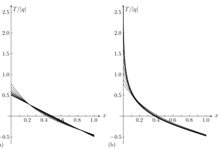
[image:12.595.88.519.81.373.2]−0.5 0.5 1.0 1.5 2.0 2.5
Figure 6: Plots of profiles of the reduced temperature T(x)/|q| in the cases (a) b= 0 (for which T(x)/|q|= 1
2 −x), 1, 2, . . . , 9 andb = bc belonging to the first family of solutions
and (b)b= 1, 2, . . . , 9 andb=bcbelonging to the second family of solutions.
problem
dw
dζ =−2 +aζ
√
w, ζ ∈(0, c),
w(c) = 0,
(4.1)
has a solution w=w(ζ) given in parametric form by
ζ =−
4 |a|
2/3 z′
(s)
z(s), w=
4 |a|
2/3 z′
(s)
z(s) 2
−s
2
, (4.2)
where
s∈[s0, si] if a >0, s∈[si, s1] if a <0, (4.3)
z is the function defined in (2.25),si is the unique positive solution of (3.2) ands1 is such that
c=
4 |a|
2/3
√si. (4.4)
It is always possible to find ans1 such that (4.4) holds since one may show that si→0 as
s1→0+ and thatsi
→ ∞ ass1→ ∞.
shows that
Iη(c) := Z c 0 2 X k=1 exp
η(−1)k Z c
ξ
ζ
p
wk(ζ) dζ
1 p
wk(ξ) dξ
=
4
a0
1/3
z(si)−4η/a0
Z s1
s0
z(s)4η/a0 ds
≍z(si)−4η/a0
sη/a0
1 exp
8η
3a0s 3/2 1
, s1 → ∞, (4.5)
where the notation f(x)≍g(x) means that f(x)/g(x) is both bounded and bounded away from 0. Integrals of the above type arose in [8] in a discussion of existence of solutions of (1.7)–(1.9); specifically, it was claimed that the function F(c) := [I1(c)]2/I2(c) satisfies F(c)∼(2πc)1/2
→ ∞ asc→ ∞. However, from (4.5) we may now assert thatF(c)≍1 as
s1 → ∞ (that is, as c → ∞), and so the claim in [8] that the equation F(c) = b1/3 has a
solution cfor any b >0 is unfounded.
5
The limit
b
→
0
+The simple solution (2.1) in the case b = 0, which is included in Figures 5(a) and 6(a), is the limit of the first family of solutions of (1.7)–(1.11) whenb →0+, since from (2.26) we
have b ∼16s3 1 →0
+ in the limit s1
→0+ and hence h(x)
→1 and T(x) → |q|(1
2 −x) for
everyx∈[0,1]. A solution for small non-zero b may be obtained as a regular expansion in
b about this solution (see Pukhnachev [14, equation (6.4)] and Karabut & Pukhnachev [8, equations (1.11), (3.1)]), and is not repeated here, for brevity.
The limit as b→0+ of the second family of solutions of (1.7)–(1.11), which corresponds
to s1→ ∞, has a more complicated structure. From (2.21), (2.27) and (A.1) we obtain
s0∼s0ˆ +π
Bi′ (ˆs0)2 2|s0ˆ | exp
−4
3s
3/2 1
, s1 → ∞, (5.1)
where ˆs0 is again the largest (negative) zero of Ai′
(s). In particular, s0 →sˆ+0 ass1 → ∞. Now Lemma A.1 and equation (A.1) yield
z(s0) = J
1/2 4 J21/2
Bi′
(s1) Ai(s0)−Ai′
(s1) Bi(s0)
∼ p
2/3π2s−1/4 1
πs−11/4 Ai(ˆs0) Bi
′ (s1)
∼ r
2π
3 Ai(ˆs0)s
1/4 1 exp
2 3s
3/2 1
. (5.2)
Hence
h(0) = 1
z(s0)2 ∼
3 2πAi(ˆs0)2s
−1/2
1 exp
−43s31/2
with b and s1 related by (2.27); thus the thickness 2h at the left endpoint x = 0 decays super-exponentially withs1. Also the curvature at this endpoint grows super-exponentially withs1 since, by (3.1)1,
h′′
(0) =−2
b
2 2/3
s0z(s0)2
∼3π|s0ˆ |Ai(ˆs0)2s−11/2exp
4 3s
3/2 1
, s1 → ∞. (5.4)
We show that, in the limitb→0+, the second family of solutions converges to the function
h0(x) = 3
2x(2−x), x∈[0,1]. (5.5)
To this end we use the substitution
s=s1−s−11/2t, 0≤t≤s31/2−s0s11/2, (5.6)
as in the proof of Lemma A.1. For fixedtwe have
z s1−s−11/2t
→
r 2
3cosht, s1→ ∞, (5.7)
by (A.2) and (A.18), which implies that
h→ 3
2 cosh2t, s1 → ∞. (5.8)
With (5.2), (5.7) and (A.17) we obtain
x=π
2
b
1/3
Ai(s0) Bi(s1−s1−1/2t)−Ai(s1−s
−1/2
1 t) Bi(s0) z(s0)z(s1−s−11/2t)
∼π2
3s
1/2 1
Ai(ˆs0)π−1/2s−1/4
1 exp
(2/3)(s1−s−11/2t)3/2
p
2π/3 Ai(ˆs0)s11/4exp
(2/3)s31/2
p
2/3 cosht
∼ cosh1 texp
2 3
(s1−s−11/2t) 3/2
−s31/2
→ e
t
cosht, s1 → ∞. (5.9)
Since
3et 2 cosht
2− e
t cosht
= 3
2 cosh2t, (5.10)
it follows from (5.8) and (5.9) that the second family of solutions of (1.7)–(1.9) converges to h0 given in (5.5) as b→0, i.e.
h(x)→ 3
2x(2−x), x∈[0,1], (5.11)
ass1 → ∞. The functionh0satisfies the differential equation (1.7), the boundary condition (1.8)2 at x = 1 and the volume condition (1.9). However, this “outer” solution does not
satisfy the boundary condition (1.8)1 at x = 0, and there is an “inner” solution in a
boundary layer near x = 0 that accommodates this boundary condition; this is in accord with the divergence ofh′′
(a)
x h
0.2 0.4 0.6 0.8 1.0 0.5
1.0 1.5
(b)
x T /|q|
0.2 0.4 0.6 0.8 1.0
[image:15.595.83.512.83.373.2]−0.5 0.5 1.0 1.5 2.0 2.5
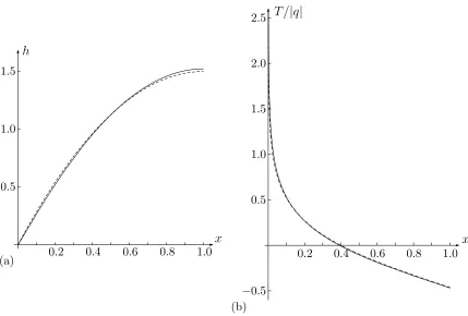
Figure 7: Plots of profiles of (a) the free surface h(x) and (b) the reduced temperature
T(x)/|q| of the second family of solutions in the case b = 1 (full curves) and the leading order outer asymptotic solutions in the limit b → 0 given by (5.11) and (5.12) (dashed curves).
In a similar way to the above one can show that the temperature converges for x∈(0,1] and diverges for x= 0:
T(x)→ |q| 3 log
2−x
4x
, x∈(0,1], (5.12)
T(0)∼ 2|q| 3 s
3/2
1 → ∞, s1→ ∞. (5.13)
Figure 7 shows comparisons between the asymptotic outer solutions forh(x) andT(x)/|q|
given in (5.11) and (5.12) and the exact solutions (2.24) and (2.9) in the caseb= 1 belonging to the second family, i.e. with s1 ≃ 3.9532 > s1c. The agreement is very good, especially since the value b= 1 is not particularly small, given that btakes values only in the interval 0≤ b≤bc ≃9.316786. Physically the solution (5.5) may be interpreted as representing a situation in which the effective Marangoni number γ is small (so that the surface tension is essentially constant) and in which the free surface has constant curvature except near
x= 0 where it distorts strongly to satisfy the contact-angle condition h′
(0) = 0. Equation (1.6)1shows that for the curvature to be non-constant near x= 0 the temperature gradient
must be large there (and so thermocapillarity is significant), and (1.6)2 shows that this is
[image:15.595.209.428.501.560.2]6
Conclusions
We have obtained a closed-form (parametric) solution of the steady two-dimensional thin-film version of a problem concerning a weightless non-isothermal free thin-film of incompressible viscous fluid subject to thermocapillarity, proposed and analysed by Pukhnachev and co-workers, and defined here in equations (1.7)–(1.11). Specifically, we extended and corrected the paper by Karabut & Pukhnachev [8] in which the problem is solved numerically, and in which it is claimed that there exists a unique solution for any value ofb. We showed that, on the contrary, solutions exist only when b≤bc≃9.316786, and that there are then two solutions, one of which recovers that obtained numerically by Karabut & Pukhnachev [8], the other being new.
The questions of why, physically, the valueb=bcis critical, and of what happens whenb > bc, remain open. It is conceivable that an unsteady evolution develops forb > bc, maintained energetically by the heat input/output at the planes x = 0 and x = 1; the equations derived by Pukhnachev & Dubinkina [15] for the unsteady situation would presumably be the starting point for an analysis of such evolutions. It is also conceivable that the steady solutions in the second family derived above are unstable; however, this is untested as yet.
We have followed Pukhnachev and co-workers in taking the film to be symmetric with respect to the plane z = 0; it would be of interest to determine whether steady non-symmetric solutions are also possible.
One advantage of having a closed-form solution is that we have been able to use it to prove that the curve in Figure 3 satisfies (a) b→0 as s1→0, (b)b has a global maximum
b = bc at s = s1c, and (c) b → 0 as s1 → ∞, and therefore that there are no “higher” branches of solutions beyond those shown in Figure 3. However, we have not been able to prove that the curve behaves monotonically on either side of its global maximum; if it does not then for some given values ofb(< bc) there will be more than two associated values of
s1, and hence there will be more than two solutions of the original problem.
The question of the possibility of the film “pinching off” when the two free surfaces come into contact is also of interest. Pukhnachev [13] showed that the solutions in the first family never approach pinch-off; this is consistent with Figure 5(a), which shows that even for the maximum valueb =bc the film is of finite thickness everywhere. We have shown that the solutions in the second family approach pinch-off only in the limit b→0, and then only at
x= 0.
A
Appendix
and their derivatives (see, e.g. [12, 9.7.5–9.7.8]):
Ai(s)∼ 1 2√πs
−1/4
exp
−23s3/2
, Ai′
(s)∼ − 1 2√πs
1/4
exp
−23s3/2
,
Bi(s)∼ √1
πs
−1/4exp
2 3s
3/2
, Bi′
(s)∼ √1
πs 1/4exp
2 3s
3/2
(A.1)
ass→ ∞. The following lemma gives the desired asymptotic behaviour of J2 and J4.
Lemma A.1. For given s1 >0 let s0 be the unique solution of (2.23)1 in (ˆs0,0). Then
J2(s0, s1)∼π2s1−1/2, J4(s0, s1)∼
2π4
3 s −1/2
1 , s1→ ∞. (A.2)
Proof. From (2.20) and (2.6) it may be shown that
J2(s0, s1) =π2Bi(s1)
Bi′ (s1) −
πBi(s0) Bi′
(s1)Bi′
(s1) Ai(s0)−Ai′
(s1) Bi(s0). (A.3)
The result forJ2 in (A.2) follows from (A.3) and (A.1), the second term in (A.3) decaying exponentially.
ForJ4 first note that
Ai(s),Bi(s),Bi′
(s)>0 and Ai′
(s)<0, s∈(ˆs0,∞). (A.4)
Using (A.4) we may estimate the integral over the negative part of the interval as follows: Z 0
s0
1
Bi′
(s1) Ai(s)−Ai′
(s1) Bi(s)4ds≤ Z 0 ˆ s0 1 Bi′
(s1) Ai(s)4 ds
= 1
Bi′ (s1)4
Z 0
ˆ
s0 1
Ai(s)4 ds≤
C s1 exp
−83s31/2
, (A.5)
which is exponentially small.
Now consider the second part of the integral. Let us define
e
J4(s1) := Z s1
0
1
Bi′
(s1) Ai(s)−Ai′
(s1) Bi(s)4 ds (A.6)
fors1>0. In this integral we make the substitutions=s1−s−11/2t, which yields
e
J4(s1) =s−11/2
Z s31/2
0
dt
h Bi′
(s1) Ai s1−s−11/2t
−Ai′
(s1) Bi s1−s−11/2t
i4 . (A.7)
We show that the integrand is uniformly bounded by an integrable function so that we may apply the Dominated Convergence Theorem. It follows from the asymptotic formulae (A.1) that there existm, M >0 such that
m(1 +s)1/4exp
2 3s
3/2
≤Bi′
(s)≤M(1 +s)1/4exp
2 3s
3/2
, (A.8)
m(1 +s)−1/4
exp
−23s3/2
≤Ai(s) ≤M(1 +s)−1/4
exp
−23s3/2
for all s∈[0,∞). Hence for 0≤t≤s31/2 we have
Bi′
(s1) Ai s1−s−11/2t
−Ai′
(s1) Bi s1−s−11/2t
≥Bi′
(s1) Ai s1−s−11/2t
≥m2(1 +s1)1/4exp
2 3s
3/2 1
1 +s1−s−11/2t
−1/4
exp
−23 s1−s−11/2t
3/2
=m2
1− t
(1 +s1)s11/2
−1/4
exp
2 3 h
s13/2− s1−s1−1/2t3/2i
≥m2exp f(s1, t), (A.10)
where use has been made of (A.4), and we have introduced the function
f(s1, t) := 2 3 h
s31/2− s1−s
−1/2
1 t
3/2i
, s1, t∈[0,∞), s1≥t2/3. (A.11)
The derivative off(s1, t) with respect to s1 is given by
∂f(s1, t)
∂s1 =s
1/2
1 − s1−s
−1/2
1 t
1/2
1 + 1 2s
−3/2
1 t
= t
2 3 +s−3/2
1 t
4s2 1
h
s11/2+ s1−s
−1/2
1 t
1/2
1 +1 2s
−3/2
1 t
i, (A.12)
showing that ∂f(s1, t)/∂s1 ≥0, which in turn implies that
f(s1, t)≥f t2/3, t= 2 3 h
t− t2/3−t−1/3
t3/2i= 2
3t for s1≥t
2/3
. (A.13)
It therefore follows from (A.10) and (A.13) that
Bi′
(s1) Ai s1−s−11/2t−Ai′
(s1) Bi s1−s−11/2t≥m2exp f(s1, t)≥m2exp
2 3t
. (A.14)
Hence the integrand in (A.7) is bounded from above by
1
m8 exp
−83t
, (A.15)
which is an integrable function. Let us consider the pointwise limit of the integrand as
s1→ ∞, i.e. for fixed t. From the asymptotic expansions in (A.1) we obtain
Bi′
(s1) Ai s1−s−11/2t
−Ai′
(s1) Bi s1−s−11/2t
∼ 21πs11/4exp
2 3s
3/2 1
s1−s−11/2t
−1/4
exp
−23 s1−s−11/2t
3/2
+ 1 2πs
1/4 1 exp
−23s31/2
s1−s−11/2t
−1/4
exp
2
3 s1−s −1/2
1 t
3/2
= 1
2π 1−s
−3/2
1 t
−1/4
exp f(s1, t)+ exp −f(s1, t)
The function f(s1, t) has the asymptotic behaviour
f(s1, t) = 2 3s
3/2 1
h
1− 1−s−13/2t
3/2i
=t+ Os−13/2
→t, s1→ ∞, (A.17)
and hence
Bi′
(s1) Ai s1−s−11/2t
−Ai′
(s1) Bi s1−s−11/2t
→ π1 cosht, s1 → ∞. (A.18)
By the Dominated Convergence Theorem we therefore obtain
lim s1→∞
Z s31/2
0
dt
h Bi′
(s1) Ai s1−s−11/2t
−Ai′
(s1) Bi s1−s−11/2t
i4 =π 4
Z ∞
0
dt
cosh4t. (A.19)
With the substitution x= e2t we have Z ∞
0
dt
cosh4t =
Z ∞
0
16e4t
1 + e2t4 dt= Z ∞
1
8x
(1 +x)4 dx=
2
3 (A.20)
and hence
lim s1→∞
Z s31/2
0
dt
h Bi′
(s1) Ai s1−s−11/2t
−Ai′
(s1) Bi s1−s−11/2t
i4 =
2π4
3 , (A.21)
which, together with (A.5) and (A.7), implies that
J4(s0, s1)∼J4e(s1)∼ 2π
4
3 s −1/2
1 , s1 → ∞. (A.22)
Acknowledgements
This work was completed while S. K. W. was a Leverhulme Trust Research Fellow (2013– 2016) supported by award RF–2013–355, “Small Particles, Big Problems: Understanding the Complex Behaviour of Nanofluids”.
References
[1] Abramowitz, M. & Stegun, I. A. (1964) Handbook of Mathematical Functions. Dover.
[2] Bonn, D., Eggers, J., Indekeu, J., Meunier, J. & Rolley, E. (2009) Wetting and spreading.Rev. Mod. Phys.81, 739–805.
[4] Duffy, B. R. & Wilson, S. K.(1997) A third-order differential equation arising in thin-film theory and relevant to Tanner’s law.Appl. Math. Lett. 10, 63–68.
[5] Eggers, J. (2004) Hydrodynamic theory of forced dewetting. Phys. Rev. Lett. 93, 094502, 4pp.
[6] Eggers, J.(2005) Existence of receding and advancing contact lines.Phys. Fluids 17, 082106, 10pp.
[7] Janeˇcek, V., Andreotti, B., Praˇz´ak, D., B´arta, T. & Nikolayev, V. S.
(2013) Moving contact line of a volatile fluid.Phys. Rev. E 88, 060404, 5pp.
[8] Karabut, E. A. & Pukhnachev, V. V. (2008) Steady-state conditions of a non-isothermal film with a heat-insulated free boundary. J. App. Mech. Tech. Phys. 49, 568–579.
[9] Karpitschka, S. & Riegler, H. (2012) Noncoalescence of sessile drops from dif-ferent but miscible liquids: hydrodynamic analysis of the twin drop contour as a self-stabilizing traveling wave.Phys. Rev. Lett. 109, 066103, 5pp.
[10] Limat, L. & Stone, H. A.(2004) Three-dimensional lubrication model of a contact line corner singularity.Europhys. Lett. 65, 365–371.
[11] Neogi, P. (2010) Bead formation near the contact line in forced spreading. Chem. Eng. Sci. 65, 4572–4578.
[12] NIST Handbook of Mathematical Functions. Edited by F. W. J. Olver, D. W. Lozier, R. F. Boisvert and C. W. Clark. U.S. Department of Commerce, National Institute of Standards and Technology, Washington, DC; Cambridge University Press, Cambridge (2010). Online version: http://dlmf.nist.gov
[13] Pukhnachov, V. V.(2002) Model of a viscous layer deformation by thermocapillary forces.European J. Appl. Math. 13, 205–224.
[14] Pukhnachev, V. V.(2007) Equilibrium of a free nonisothermal liquid film. J. App. Mech. Tech. Phys.48, 310–321.
[15] Pukhnachev, V. V. & Dubinkina, S. B. (2006) A model of film deformation and rupture under the action of thermocapillary forces.Fluid Dynamics 41, 755–771.
[16] Snoeijer, J. H. & Andreotti, B.(2013) Moving contact lines: scales, regimes, and dynamical transitions.Annu. Rev. Fluid Mech.45, 269–292
[17] Tuck, E. O. & Schwartz, L. W.(1990) A numerical and asymptotic study of some third-order ordinary differential equations relevant to draining and coating flows.SIAM Review 32, 453–469.


![Figure 4: Typical plot of zs as a function of s ∈ [s0, s1], in the case s1 = 2.7, for which0 ≃ −1.01722.](https://thumb-us.123doks.com/thumbv2/123dok_us/1585743.111227/10.595.140.465.91.292/figure-typical-plot-zs-function-s-case-which.webp)