Estimating fault numbers remaining after testing

Estimating Fault Numbers Remaining After Testing

Marc Roper

Dept. Computer and Information Sciences University of Strathclyde

Glasgow, UK [email protected]

Abstract—Testing is an essential component of the software development process, but also one which is exceptionally difficult to manage and control. For example, it is well understood that testing techniques are not guaranteed to detect all faults, but more frustrating is that after the application of a testing technique the tester has little or no knowledge of how many faults might still be left undiscovered. This paper investigates the performance of a range of capture-recapture models to determine the accuracy with which they predict the number of defects re-maining after testing. The models are evaluated with data from two empirical testing-related studies and from one larger publicly available project and the fac-tors affecting the accuracy of the models are analysed. The paper also considers how additional information (such as structural coverage data) may be used to improve the accuracy of the estimates. The results demonstrate that diverse sets of faults resulting from different testers using different techniques tend to produce the most accurate results, and also illustrate the sensitivity of the estimators to the patterns of fault data.

Keywords-Testing, Fault Estimation, Capture-Recapture

I. Introduction

Testing is an essential component of the software development process, but also one about which we have limited knowledge. The large number of theoretical in-sights do not necessarily translate into practice. A major deficiency is the lack of quantitative information about the effectiveness of testing. Having tested a piece of software, the software engineer is still uncomfortably in the dark — how effective has the process been, and how many faults are left?

This paper seeks to address the problem of test effec-tiveness by using capture-recapture techniques to make estimates of how many faults are remaining in a piece of software after it has been tested. Capture-recapture techniques are used within fields such as population ecol-ogy and essentially look at the overlap and distinctive-ness between samples to make estimates about the total population. A number of models have been developed for capture-recapture techniques, and these are evaluated using fault data drawn from two experiments to compare

different testing techniques and a larger publicly avail-able software system with a large associated pool of test suites. In this study the faults discovered in a program by two independent testers are used as input to the different estimators for the models in order to calculate the predicted total number of faults in the program. Since the total number of faults is known in all cases the accuracy of the predictions can be evaluated. This not only provides valuable information about how many faults are yet to be discovered, it also gives an indication of the effectiveness of testing. This information may then be used to make decisions regarding the need for more testing or to formulate risk assessments associated with the software under development.

II. Background and Related Work

A. Capture-Recapture Techniques

Capture-recapture techniques are used extensively by the biological community to make estimates of the population size of a particular species within an area. A number of traps are laid for an animal which are then inspected after a period of time. The number of animals trapped is counted and the animals are marked and released. The traps are then reset, and the process repeated. On the second trapping the biologist might find that some new animals are caught along with those which were captured previously. Several iterations of this process of trapping and releasing might occur, and at the end the biologist has information about numbers of animals and how many times they have been trapped. In a given area, some animals might be trapped several times whilst others might never be trapped. This data is then used as input to capture-recaptur models to make predictions about the total population in the area.

B. Capture-Recapture Models

Capture-recapture models make various assumptions about the environment from which their data is drawn. These are:

1) The population is closed. That is, no animals enter or leave the area, or are born or die during the time that trapping occurs.

3) All marks are correctly noted and recorded. 4) Each animal has a constant and equal probability

of capture on each trapping occasion.

This final assumption might seem prohibitively strict, and in practice is not met in most studies. The relaxation of this assumption leads to the three possible sources of variation in capture probability outlined below (where M stands for Model):

Mt Probability varies with time, or trapping

occa-sion. This might occur due to such influences as weather conditions (which effects the animals’ behaviour) or the use of different capture meth-ods.

Mb The probability of capture varies according to

behavioural responses. That is, an animal’s be-haviour becomes altered after its initial capture (e.g. it becomes trap happy or shy).

Mh The probability of capture varies according to

the individual animal (i.e. heterogeneity of the population). This might be due to different animal behaviour, social status etc.

It is also possible to consider combinations of the above models. For example, Mtb represents the model where

both time and behaviour effect the probability of cap-ture. There is also the Null case (M0) where assumption 4 above is met. For more details on the fundamental ideas the reader is guided towards the work of Otis et al. [1] or Chao and Lee [2].

C. Applications in Software Engineering

Capture-recapture techniques have been applied to software engineering problems for many years. Whilst the exact adaptation of the concepts outlined above varies with the application area, some generalisations are possible: an animal equates to a defect or fault of some sort, the population size is the total number of defects, and the trapping method is the means by which the defect is detected. The precise adaptation of the models to this study is explained in section III-C.

The use of capture-recapture techniques to predict numbers of missing defects after testing was originally made by Mills [3]. Pseudo defects were seeded into a program which was then tested. The tester reported the number of defects found and these would include pseudo defects and real defects. These two sets of defects were then used as input to the Lincoln-Petersen estimator (see section III-C). In a study similar to this, Basin [4] also used the Lincoln-Petersen estimator but drew defects from two testers. Since these studies were carried out a number of new estimators have been developed and the work reported here evaluates these new estimators and also considers the impact of using different testing techniques.

Stringfellow et al. [5] explored the use of capture-recapture techniques in testing to make predictions about the likelihood of components being faulty after release even if they did not appear faulty when tested. The focus here is slightly different as the goal is not to make estimates about total fault numbers but to identify the numbers of faulty components in a system given the numbers that exhibited failures in the testing phase. The application of the technique is explored via a case study using data from varying numbers of sites.

Yang and Chao [6] investigated the use of “recapture debugging” which looks at the overlap between root causes of failures to make decisions about when to stop testing. This, and other models, were evaluated using simulated scenarios derived from real data. Again the focus is not to determine precise numbers of faults.

Scott and Wohlin [7] employed an industrial case study to explore the viability of using capture-recapture techniques to predict numbers of failures after unit testing. The study was fairly small-scale, with four de-velopers, a total of five observed failures and just one model evaluated using the range of developer combina-tions. However, the approach was deemed to be both cost-efficient and appropriate, and generated estimates that were comparable with the subjective ones of the participants.

Capture-recapture techniques have been widely ex-plored in the software inspection domain, again to pre-dict fault content after reviews have been carried out (see, for example the work of Eick et al. [8], Vander Weil and Votta [9], Wohlin et al. [10] or Briand et al. [11]). The application here is quite natural as inspectors auto-matically carry out an independent review of a document as part of the process, and the faults found by these individual reviewers may then be fed into the models to make predictions about the total number of faults in the document or piece of software under review. The large number (relatively speaking) of reviewers involved allows for more accurate estimates to be made. Both Briand et al. [12] and Petersson et. al [13] provide very comprehensive reviews of the application of capture-recapture techniques within the inspection domain and the results of evaluating various models.

III. Background to the Models

A. Mapping to Testing Domain

One of the primary concerns here is what constitutes a trapping occasion, and how many trapping occasions should be considered (the necessity for recapture obvi-ously implies that this should be more than one!). A trapping occasion is the application of a testing tech-nique to a program by an individual. Any subsequent trapping occasions have to be carried out by a different tester (to repeat the process with the same tester, even using a different technique, would be flawed – the tester simply has too much knowledge of some of the faults in the program).

B. How Many Testers?

Studies in the inspections and reviews domain often consider between 2 and 6 reviewers. Reviews are known to be expensive, but their benefits are well understood and so the idea of employing multiple people to perform the same task is not unreasonable in this context. The cost-benefits of testing are less well understood. A previ-ous study [14] showed that an individual using a testing technique finds on average around 56% of all faults. Creating hypothetical pairings of testers raises this figure to around 73%. Employing three testers would raise this again to around 79%. From this it would appear that the cost of employing two testers is not unreasonable considering the benefits of improved fault detection cou-pled with the opportunity to predict how many faults remain undetected. The argument for employing three testers is less convincing, so for this reason the studies in the paper are restricted to two trapping occasions (i.e. two independent testers).

C. Models Selected and Estimators

When applying capture-recapture techniques to a field such as testing the first thing to consider is which assumptions are met and to identify the sources of varia-tion in probability, as it is these factors which determine the applicability of the models.

Considering the four assumptions in section II-B, the first assumption is met if the code is not altered whilst under test (i.e. faults are neither removed nor introduced). The second and third assumptions are met if faults discovered are carefully recorded. The fourth assumption is unlikely to be true. Many empirical studies have shown that faults are not evenly distributed in the sense that they have an equal probability of capture, and everyday experience bears this out. This last fact rules out the application of modelM0.

There are a number of sources of variation in prob-ability of capture. The fact that the process involves two different testers is one source of variation. The application of a testing technique is dependent on the person doing the testing – different people choose differ-ent data. Furthermore, the use of a differdiffer-ent technique

(i.e. functional or structural) is also a source of variation. In fact it is difficult to separate out these two sources of variation as the test data produced is a combination of tester and technique. The second source of variation is that already discussed in the previous paragraph - the heterogeneity of faults.

For these reasons it was decided to investigate three models:

Mt This assumes that the probability of fault

de-tection differs between techniques/testers. Mh This assumes that the probability of fault

de-tection differs between faults.

Mth Which combines the above so that both

the faults and the techniques/testers become sources of variation.

It was decided that the application of any models which took into account behaviour were inappropriate. Faults do not have behaviour patterns per se, and whilst their capture might effect the probability of other faults being captured (a bug has been found and the tester might modify their strategy), it does not alter the prob-ability of their “subsequent” capture (i.e. their discovery by an independent tester). For this reason, noMbmodels

were considered.

For each of the above models a number of estimators have been developed (and continue to be developed) for calculatingN - the total population. These are outlined below along with the formula. It must be noted that the formula here are for the cases wheret= 2 (i.e. there are two trapping occasions - or samples - or testers) for the reasons outlined in section III-A. The more general forms of the estimators may be found in papers describing the principles of the approaches such as Otis et al. [1] or Chao and Lee [2] or in the appendix of the study of Stringfellow et al. [5].

1) Estimators forMt: The simplest estimator for this

model is known as the Lincoln-Petersen estimator [1] and is defined as

ˆ

N= n1n2 m1

where n1 is the number caught in the first sample, n2 is the number caught in the second sample, and m1 is the number caught in both (i.e. the overlap between the samples).

Lee and Chao [2] define an estimator for this model as

ˆ

N =D/Cˆ

whereDis the number of distinct animals (faults) caught in the two samples, and

ˆ

C= 1−_Ptf1

k=1kfk

times int samples (so in this case the number of faults that were detected exactly once or twice are considered). 2) Estimators for Mh: Burnham and Overton [15]

proposed the Jackknife estimator for this model. For the special case oft= 2 considered here this can be defined as

ˆ N =D+

_t−1

t

f1

whereD, tand f1 are as defined above.

Chao [16] proposed an estimator for this model which attempts to address a reported deficiency of the Jack-knife model (Chao suggests that it does not perform well when the data is skewed and captured animals are mostly caught once or twice). The definition of this is

ˆ

N=D+f₁2/2f2

Lee and Chao [2] also define an estimator for this model but it is essentially the same as the estimator for Mth discussed next.

3) Estimators for Mth: The only estimator used for

this model is again proposed by Chao and defined in Lee and Chao [2] as

ˆ N =D

ˆ C +

A ˆ Cγ

2

where A = f1 and γ2 _{represents an estimator for the} coefficient of variation of the capture probabilities and is defined as

γ2=max{D/CˆX

k

k(k−1)fk/[2 X

j<k X

njnk]−1,0}

IV. Experimental Evaluation of the Models

This study aimed to explore the accuracy of the various estimators for predicting the total numbers of faults in a piece of software and also set out to identify the various strengths and weaknesses of the models in order to gauge their practical applicability.

A. Data Sets

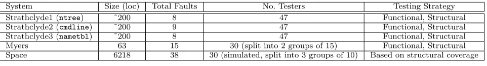
The models were evaluated using three sets of data: two were drawn from available data from testing ex-periments where faults found by participants in the studies were recorded and could then be used to create hypothetical pairings of individual independent testers, and one from publicly available system with a very large pool of test suites with associated fault revealing capabilities, which again could be used to create hypo-thetical pairings. These are described in detail below and summarised in Table I.

1) The Strathclyde Data: One set of data for this study is drawn from a previous experimental study carried out with the Department of Computer Science at Strathclyde which compared different defect detection techniques in terms of their effectiveness (percentages of failures observed and faults isolated). Further details of the original experiment may be found in Wood et al. [17]. The programs used in the experiment were taken from a replication package produced by Kamsties and Lott [18]. The programs were written in C and were approximately 200 lines long (excluding blank lines and comments). The first program,ntree, implemented an abstract data type, namely a tree with unbounded branching. The second program, cmdline, basically displayed the result of parsing a command line. The third program,nametbl, implemented another abstract data type, namely a sim-ple symbol table.

The faults within the programs were those provided with the replication package. These faults were mostly seeded by Kamsties and Lott, although it is understood that a few original developer faults are included. The faults were chosen so that programs fail on some inputs only, where a failure may result in no output at all, incorrect output, or a minor problem such as misspelling. There were 8 faults in total in thentreeprogram, 9 in thecmdline program, and 8 in thenametblprogram.

The fault detection techniques were applied in a two stage process. Firstly, failures were observed, that is the subject looked for observable differences between the program and the specification. Secondly, faults were isolated, that is the subject attempted to identify the exact location of the cause of failure in the program code.

The three defect detection techniques used were:

• Code Reading: This used the technique of stepwise abstraction [19], but the results are not used within the context of this study.

• Functional Testing: This was based on the standard techniques of equivalence partitioning and bound-ary value analysis [20]. Subjects were initially pro-vided with an on-line executable version of the program code and a program specification. Tests cases were derived from the specification, run using the executable, and failures observed in terms of unexpected results.

System Size (loc) Total Faults No. Testers Testing Strategy

Strathclyde1 (ntree) ˜200 8 47 Functional, Structural

Strathclyde2 (cmdline) ˜200 9 47 Functional, Structural

Strathclyde3 (nametbl) ˜200 8 47 Functional, Structural

Myers 63 15 30 (split into 2 groups of 15) Functional, Structural

Space 6218 38 30 (simulated, split into 3 groups of 10) Based on structural coverage

Table I

Summary of data sets used in evaluation of the models

Each subject applied each technique to three pro-grams. The design was balanced so that subjects never used the same program twice and each technique was applied with approximately equal frequency to each program. The 47 subjects were honours students enrolled in a practical software engineering class at the University of Strathclyde. The subjects had all completed two years of programming classes (including classes in C programming). Prior to the experiments the students were given lectures on each of the fault finding tech-niques together with three 2-hour, supervised training sessions to practice applying each of the techniques. The dependent variables examined in the study were the number of failures observed, the number of faults detected, the time taken to observe failures and the time taken to isolate faults. In the context of this study, it is the data concerning the faults detected that is used.

2) The Myers Data: Myers [21] ran an experiment to compare team-based code “walkthroughs/ inspec-tions” with individuals using variations of structural and functional testing. Myers’ experiment used 59 pro-fessional programmers (averaging 11 years experience) split into three groups, each group using one technique. The experiment was based on one PL/I program - the renowned Naur ‘text formatter’ - containing 15 defects. The techniques are basically similar to those carried out at Strathclyde (the walkthrough data was also ignored) except that those employing structural testing made use of the specification as well as the code (in the Strathclyde study, structural testers were givenonlythe code initially). The Myers data is contained within the original paper.

3) The Space Data: Space is one of the systems con-tained within the Software-artifact Infrastructure Repos-itory (SIR) [22] which acts as as an interpreter for an array definition language and consists of 9564 (6218 executable) lines of C. Within the SIR is the original version of the program containing 38 naturally occurring faults along with 13,585 test cases and a fault matrix which identifies which of the 38 faults are revealed by each of the test cases. In addition, the test cases have been collected into pools of 1000 test suites, where the suites in each pool have been established to achieve a particular level of coverage of the entire program: the

ones employed in this study are “minimum-statement”, “statement” ( “minimum-statement” but augmented with additional tests), and “random”. The suites in each pool are unique but not entirely independent (i.e. some test cases appear in more than one suite) and contain varying numbers of test cases (between 62 and 76 for “minimum-statement”, 79 to 105 for “statement” and 140 to 170 for “random”). By treating each test suite as the product of an individual tester, this set-up provides the opportunity to explore the effectiveness of the estimators on a larger system. Subsets of ten suites were randomly chosen from each of the pools (theSpaceprogram also contains a list of random numbers for selecting test suites).

B. Method

The five estimators for the three models outlined above were evaluated using the fault data revealed by each of the tests (either real or simulated). For each program every possible pairwise combination of testers was considered for both an individual technique (i.e. just combining the results from structural testing or func-tional testing) and combined techniques (i.e. combining a functional and a structural tester) where possible. This created hypothetical pairings of individual, independent testers, and the faults discovered by each of these pairs was fed into the models. As mentioned earlier only combinations of two testers are explored initially, unlike studies in reviews and inspections which often explore using the data from up to five or six individuals.

V. Results and Analysis

a relatively small spread of values. The boxplots are labelled to indicate which model is being applied with which testing technique to which program. The model estimator names prefix the labels and are defined as:

LP Lincoln-Peterson estimator for Mt

JK Jackknife estimator forMh

CMT Chao estimator for Mt

CMH Chao estimator for Mh

CMTHChao estimator for Mth

Included in the names are the testing technique identi-fiers (again, if relevant) which are:

FT Functional testing ST Structural testing

BT Both techniques, i.e. functional and structural testing combined.

The final part of the label is the program identifier (where applicable).

The results for the Strathclyde data and the Myers data are presented together because they have strong parallels since both involved real testers employing a range of testing techniques. The Space results are dif-ferent as they involve simulations based upon pools of test suites and are presented separately.

A. The Strathclyde and Myers Results

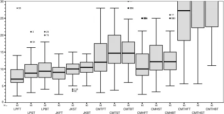
The Strathclyde results are summarised in the three sets of boxplots shown in Figures 1, 2 and 3 (one for each program). The result from the Myers data is shown in Figure 4.

80 80 80 80 80 80 80 80 80 80 80 80 80 80 80 N = CMTHBTP1 CMTHSTP1 CMTHFTP1 CMHBTP1 CMHSTP1 CMHFTP1 CMTBTP1 CMTSTP1 CMTFTP1 JKBTP1 JKSTP1 JKFTP1 LPBTP1 LPSTP1 LPFTP1 20 18 16 14 12 10 8 6 4 2 0 2 76 103 7 24 69 66 29 33 32 28 38 2 37 30 18 63 65 39 36 15 35 69 66 2 29 32 28 33 38 37 30 18 65 63 39 36 15 35 33 28 38 2 32 29 39 36 15 35 29 76 12 103 72 63 28 65 29 33 2 38 32 18 39 36 35 15

Figure 1. Values of Estimators for Program1 (N=8)

In some of the boxplots the full spread of data is not visible. This is because the data goes off the scale of the plot, and represents an estimate which is highly inaccu-rate. Rather than adjust the plot to accommodate the full range of data it was decided to focus on those plots which were closer to the desired outcome (remember that the actual values ofN are 8, 9 and 8 for the three Strathclyde programs respectively, and 15 for the Myers program). 91 91 91 91 91 91 91 91 91 91 91 91 91 91 91 N = CMTHBTP2 CMTHSTP2 CMTHFTP2 CMHBTP2 CMHSTP2 CMHFTP2 CMTBTP2 CMTSTP2 CMTFTP2 JKBTP2 JKSTP2 JKFTP2 LPBTP2 LPSTP2 LPFTP2 20 18 16 14 12 10 8 6 4 2 0 29 62 48 65 36 40 56 62 58 62 29 48 56 62 58 64 50 54 68 51 34 20 58 62 56 45 17 51 79 2 34 20 30 74 8 5 28 63 47 59 38 60 62 58 56 88

Figure 2. Values of Estimators for Program2 (N=9)

118 118 118 118 118 118 118 118 118 118 118 118 118 118 118 N = CMTHBTP3 CMTHSTP3 CMTHFTP3 CMHBTP3 CMHSTP3 CMHFTP3 CMTBTP3 CMTSTP3 CMTFTP3 JKBTP3 JKSTP3 JKFTP3 LPBTP3 LPSTP3 LPFTP3 20 18 16 14 12 10 8 6 4 2 0 23 38 64 41 20 105 57 37 101 47 44 65 58 99 45 18 31 75 66 77 55 61 4 60 63 64 56 59 62 63 108 13 103 27 36 23 64 20 105 57 41 38 77 66 55 63 60 4 62 61 56 64 59 13 63 108 36 103 27 8 39 55 5 25 23 56 6 80 85 8 116 89 117 69 86 84 104 24 118 36 52 100 71 7 119 87 55 39 23 20 64 105 41 101 37 38 57 5 25 54 35 17 67 16 18 22 32 29 42 30 19 31 68 47 44 43 65 58 34 46 75 99 92 55 85 80 81 79 83 82 6 78 20 76 33 45 77 66 57 108 27 36 63 103 13

Figure 3. Values of Estimators for Program3 (N=8)

As can be seen from the boxplots, the Chao estima-tor for Mth has a tendency to both overestimate and

generate a large spread of data (i.e. the predictions are also likely to be inaccurate). In fact, this spread is also a feature of the Chao estimators for modelsMtandMh,

but not quite so pronounced. The reason for this is that all these estimators are susceptible to large differences between the values of f1 and f2 (i.e. when there is a small amount of overlap) relative to the total number of distinct defects. For the Mt estimator, an overlap of

less than about 25% of D(the number of distinct faults

95 95 95 95 95 95 95 95 95 95 95 95 95 95 95 N = CMTHBT CMTHST CMTHFT CMHBT CMHST CMHFT CMTBT CMTST CMTFT JKBT JKST JKFT LPBT LPST LPFT 30 25 20 15 10 5 0 110 33 77 114 71 25 106 81 110 33 77 118 82 70 20 54 3 55

found) results in a predicted value forN of many times D. A similar pattern occurs for the Mh estimator at

around the 20% level. The Mth estimator is effectively

theMtestimator with an additive factor, and so displays

similar, but more exaggerated behaviour, to Mt. This

small overlap might occur when two testers are employ-ing very disparate techniques which tend to discover very different faults, or when they have very different abilities. This overestimation is most pronounced in the results for the Strathclyde data using programs 1 and 2. It is less apparent in program 3 because there is a greater overlap between the samples. With regard to the Myers data, this overestimation is far less pronounced, and the most accurate estimates are from the ChaoMtestimator using

both techniques (i.e. one functional tester and one struc-tural tester). This is a reflection of the different processes operating in the Myers and Strathclyde experiments. As noted previously, Myers provided his structural testers with a copy of the specification in addition to the code (the Strathclyde subjects only had the code). Given that both the functional testers and the structural testers were both using the specification (albeit in different ways), there is bound to be some duplication in the defects found by the two groups. This duplication then translates into an overlap between defects.

The Lincoln-Peterson estimators produce less of a spread of data but have a tendency to underestimate (anything other than the smallest overlap tends to quickly drive down the value of the estimate). Whilst the model is tolerant to a low overlap between samples and does not tend to overestimate, a relatively large overlap between samples leads to underestimation. This would suggest that it is not suitable for cases where similar faults are found by different testers. This tendency is evident in both the Strathclyde and the Myers data.

The Jackknife estimator tends to underestimate slightly when there is a small number of faults found with a high overlap. Although a little on the conservative side (the value of the estimator varies linearly betweenD and 1.5×D), the most consistently accurate estimator for all three programs in the Strathclyde study is the Jackknife estimator using two different techniques (i.e. one tester uses structural testing and the other uses functional testing). With the Myers data this estimator tends to underestimate greatly - again this is a function of the different process employed which results in both a relatively high overlap between faults coupled with a fairly low defect rate — the version of structural testing employed found between 2 and 9 faults (average 5.4) and functional testing found between 1 and 7 faults (average 4.5).

B. The Space Results

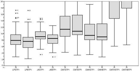
The randomly selected of test suites were treated in the same way as the efforts of individual testers and estimator values were calculated for each pairwise combination within the suite for each different coverage level suite (min-statement, statement, and random). The results for theSpacesystem are shown in Figure 5. These are grouped by estimator and labelled with one of the following suffixes indicating from which pools the test suites were drawn:

MS Min-statement

S Statement

R Random

Figure 5. Values of Estimators for Space for different test suites

The similarity between the results for the estimators for the three different test suites is noticeable — all estimators tend to underestimate, exhibit a small range of values, and tend to follow the same relative pattern with the best estimates (by a small margin) coming from the test suites with the highest level of coverage (statement), followed by those derived from the min-statement test suites and then by the those from the random test suites (even though these contained by far the largest numbers of test cases). Both the Jackknife estimator and the ChaoMt estimator are very similar.

The Lincoln-Peterson and ChaoMh estimators are also

similar and generate the largest underestimates. Only the Chao Mth estimator demonstrates an appreciable

in random. These two factors combined result in a high overlap between the suites and serves to explain both the small range of values and the persistent underestimation.

VI. The Impact of Test Coverage Data

A common measure used to determine the amount of testing done (or to direct the testing in some way) is structural coverage. There are a large number of coverage measures in use, based on criteria such as the structure of the program or the way it manipulates its data. The proportion of coverage assiciated with a pro-gram is obviously going to have an impact on the defects found within the program (by the simple argument that if a defect lies in an untested part of the code, then it is unlikely to be revealed by testing). However, the relationship is not simple and the counter-argument does not hold - a piece of code containing a defect may be executed, but the defect will not necessarily be revealed. For all the Stratchlyde sets of data, the level of branch coverage achieved was available. This data was used to make a simple modification to the estimate by increasing it in proportion to the amount of coverage achieved (e.g. an estimate based on 50% coverage was doubled). This is a very simplistic scaling factor and assumes that all defects are uniformly distributed. The modified results from the estimators are shown in Figures 6, 7 and 8

98 98 98 98 98 98 98 98 98 98 N = CMTHBTP1 CMTHSTP1 CMHBTP1 CMHSTP1 CMTBTP1 CMTSTP1 JKBTP1 JKSTP1 LPBTP1 LPSTP1 20 18 16 14 12 10 8 6 4 2 0 117 14 12 72 44 29 7 103 76 12

Figure 6. Values of Estimators for Program1 Using Coverage

Information

The results of this modification tend to increase the value of the median (and hence the accuracy of the results, since most estimators tended to underestimate) and slightly increase the spread of data. The reason for this is partly to do with the complicated relationship between coverage and fault detection. In all programs the majority of subjects achieved between about 80% and 95% branch coverage, but the number of faults found varied between 1 and 7, and there was not a strong correlation between coverage and fault detection. This approach could be a reasonable way of improving estimate accuracy, but also one which requires more

91 91 91 91 91 91 91 91 91 91 N = CMTHBTP2 CMTHSTP2 CMHBTP2 CMHSTP2 CMTBTP2 CMTSTP2 JKBTP2 JKSTP2 LPBTP2 LPSTP2 20 18 16 14 12 10 8 6 4 2 0 48 62 56 62 58 58 20 34 28 47 59 58 56 29 40 34 20 30 47 28 59 58 56

Figure 7. Values of Estimators for Program2 Using Coverage

Information 118 118 118 118 118 118 118 118 118 118 N = CMTHBTP3 CMTHSTP3 CMHBTP3 CMHSTP3 CMTBTP3 CMTSTP3 JKBTP3 JKSTP3 LPBTP3 LPSTP3 20 18 16 14 12 10 8 6 4 2 0 85 69 117 23 38 64 20 57 105 41 44 85 66 18 31 77 55 59 64 56 4 60 62 61 63 23 38 64 20 41 105 57 66 18 31 77 55 25 5 62 63 61 57 38 64 20 41 105 57 101 37 5 25 58 44 65 77 57

Figure 8. Values of Estimators for Program3 Using Coverage

Information

knowledge about the nature of faults and the effect of coverage than is currently available.

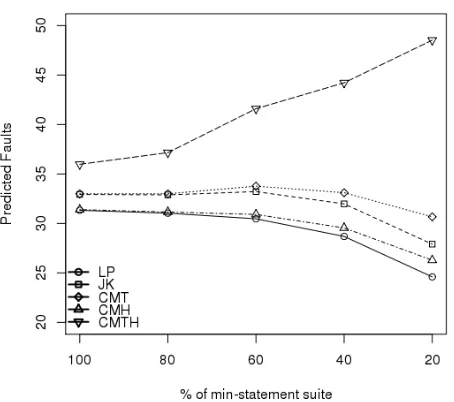
Since coverage levels for the Space system where already at 100% (statement coverage) it was decided to explore the impact of reducing levels of coverage. Most industrial systems typically don’t achieve a level of anywhere near 100% statement coverage so exploring the accuracy of the various estimators at lower levels of coverage can provide valuable insights into the practical application of these techniques. This was achieved by randomly pruning test cases from the min-statement pool of 10 suites to leave just 80% of the test cases (approximating to 80% coverage). This process was re-peated to yield suites containing 60%, 40% and 20% of the original test cases. The value of the estimators were then calculated in the same way as for the original estimates (by investigating all pair-wise combinations), and the results are illustrated in Figure 9 and shown in more detail in Table II (in which the row labelled ‘Fault range and mean’ indicates the range of faults detected for each proportion of the dataset followed by the mean number of faults detected).

Proportion of original data suite (%)

100 80 60 40 20

Fault range and mean [28-32] (30) [28-32] (29.3) [25-31] (27.5) [23-29] (24.7) [17-22] (18.9)

LP 31.33 (0.85) 31.04 (0.9) 30.47 (1.3) 28.69 (2.17) 24.6 (2.42)

JK 32.93 (1.39) 32.89 (1.35) 33.22 (1.74) 31.98 (2.67) 27.91 (2.95)

CMT 33.0 (1.52) 33.0 (1.52) 33.77 (2.14) 33.11 (3.34) 30.67 (4.3)

CMH 35.98 (3.42) 37.16 (3.39) 41.6 (5.86) 44.22 (7.65) 48.53 (11.25)

CMTH 31.4 (0.96) 31.16 (1.02) 30.91 (1.35) 29.55 (2.39) 26.29 (3.1)

Table II

Mean(SD) estimator values for decreasing proportions of the SPACE min-statement suite

Figure 9. Plot of mean values of estimator values for decreasing

proportions of the min-statement suite

sizes of test suites — the Chao Mt estimator in

partic-ular. It is also noticeable how the Chao Mth estimator

veers out of control in a different direction to all the others, quickly generating overestimates along with a disproportionately large standard deviation. This is in line with the findings from the earlier studies and is caused by the steadily falling overlap between faults as the size of the test suite drops. However, it is clear that the Space results for different coverage level can not be scaled in the same na¨ıve way as was explored with the Strathclyde data as this would lead to gross over-estimation for the lower levels of coverage.

VII. Study Limitations

This study naturally contains a number of threats to validity, particularly concerning the generalisation of the results. The findings provide some useful insights into the application of the technique but more studies

are required to explore this further and provide further evidence. The programs used in the tester-related studies were relatively small (around 200 lines of C in the Strathclyde study and 63 lines of PL/I in the Myers study) and contained quite disproportionate numbers of faults - the Myers program being far more densely populated than the Strathclyde one. Furthermore the participants in the Strathclyde study were students.

It is also worth mentioning that the Space data may well not be representative. There are clearly a substantial proportion of the faults (around 50%) that are easily caught by a small proportion of tests. This amount of “low-hanging fruit” may well not be typical of all pro-grams. There are also 5 faults which are never detected, leaving the remainder to be susceptible to differing levels of coverage.

Another factor in the study is that only subsets of 10 test suites were chosen for Space. This could easily be expanded since for each of the levels of coverage there are a thousand test suites. However, from an initial investigation they all tend to yield similar numbers of faults to those (randomly) selected for the study, so the value of extending this study to incorporate more test suites is questionable.

VIII. Conclusions and Further Work

This study has evaluated a number of capture-recapture models using fault data to predict the number of faults remaining in a program after module testing. The findings from the various studies illustrate that while capture-recapture techniques can be applied to make reasonably accurate estimates of remaining faults, the performance of the models tends to vary between datasets.

For the Strathclyde data the Jackknife estimator using data from testers using different techniques produces the best results. For the Myers data the Chao Mt

estima-tor has the best median value (using both techniques again) but a larger variance. For the Space data the Chao Mth estimator on the structural test suites again

slight underestimator, has a similar median to the Chao Mt estimator but a smaller variance.

These findings illustrate the estimators’ susceptibility to the data being used – in particular the pattern of over-lap and distinctiveness between faults. In practical terms this translates into careful application of the process used to generate the fault-revealing test data. The results from the studies suggest that the diversity generated by different testers using different testing approaches are likely to generate the most accurate results. However, too muchdiversity with respect to the overlap amongst faults may also lead to inaccurate estimates.

Results from the reviews and inspections domain are similar with the Jackknife typically producing the most accurate estimates. However, Briand et al. [11] argue that the models should not be used with less than four inspectors as the results tend to become highly variable. Whilst this is a reasonable stance to take with inspec-tions (which are in many cases a group activity, and also a process which has been economically justified), it is not one which is likely to be cost effective in the testing domain. Given that the number of testers cannot be reasonably increased above two, alternative means have to be found for increasing the accuracy of the estimates. One possibility is to augment the test data created by testers with randomly generated or evolved data and using this to take the place of additional testers. This is something to be explored in future work.

References

[1] D. L. Otis, K. P. Burnham, G. C. White, and D. R. Anderson, “Statistical inference from capture data on closed animal populations,”Wildlife Mongraphs, vol. 62, 1978.

[2] A. Chao and S. Lee, “Estimating population size via sample coverage for closed capture-recapture models,”

Biometrics, vol. 50, 1990.

[3] H. Mills, “On the statistical validation of computer programs,” IBM Federal Systems Division, Tech. Rep. Technical Report FSC-72-6015, 1972.

[4] S. L. Basin, “Estimation of software error rates via capture-recapture sampling,” Science Applications Inc., Tech. Rep., 1973.

[5] C. Stringfellow, A. A. Andrews, C. Wohlin, and H. Pe-tersson, “Estimating the number of components with defects post-release that showed no defects in testing,”

Softw. Test., Verif. Reliab., pp. 93–122, 2002.

[6] M. Yang and A. Chao, “Reliability-estimation and stopping-rules for software testing, based on repeated appearances of bugs,”Reliability, IEEE Transactions on, vol. 44, no. 2, pp. 315 –321, jun 1995.

[7] H. Scott and C. Wohlin, “Capture-recapture in software unit testing: a case study,” inProceedings of the Second ACM-IEEE international symposium on Empirical software engineering and measurement, ser. ESEM ’08.

New York, NY, USA: ACM, 2008, pp. 32–40. [Online]. Available: http://doi.acm.org/10.1145/1414004.1414012 [8] S. G. Eick, C. R. Loader, M. D. Long, L. G. Votta, and S. V. Weil, “Estimating software fault content before codeing,” inProceedings of the 14th International Con-ference on Software Engineering, May 1992, pp. 59–65. [9] S. V. Weil and L. Votta, “Assessing software designs

using capture-recapture methods,” IEEE Transactions on Software Engineering, vol. 19, no. 11, pp. 1045–1054, November 1993.

[10] C. Wohlin, P. Runeson, and J. Brantestam, “An exper-imental evaluation of capture-recapture in software in-spections,”Software Testing, Verification and Reliability, vol. 5, pp. 213–232, 1995.

[11] L. Briand, K. E. Emam, B. Freimut, and O. Laiten-berger, “Quantitative evaluation of capture-recapture models to control software inspections,” in Proc. 8th International Symposium on Software Reliability, 1997, pp. 234–244.

[12] ——, “A comprehensive evaluation of capture-recapture models for estimating software defect content,” Fraun-hofer Institute for Experimental Software Engineering, Tech. Rep. International Software Engineering Network Technical Report ISERN-98-31, 1998.

[13] H. Petersson, T. Thelin, P. Runeson, and C. Wohlin, “Capture-recapture in software inspections after 10 years research–theory, evaluation and application,”Journal of Systems and Software, pp. 249–264, 2004.

[14] M. Roper, M. Wood, and J. Miller, “An empirical eval-uation of defect detection techniques,”Information and Software Technology, vol. 39, pp. 763–775, 1997. [15] K. Burnham and W. Overton, “Estimation of the size

of a closed population when capture probabilities vary among animals,”Biometrika, vol. 65, 1978.

[16] A. Chao, “Estimating the population size for capture-recapture data with unequal catchability,”Biometrics, vol. 45, 1987.

[17] M. Wood, M. Roper, A. Brooks, and J. Miller, “Com-paring and combining software defect detection tech-niques:a replicated empirical study,” in Proceedings of The Sixth European Software Engineering Conference, H. S. Mehdi Jazayeri, Ed., vol. 1301. Lecture Notes in Computer Science, September 1997, pp. 262–277. [18] E. Kamsties and C. Lott, “An empirical evaluation of

three defect detection techniques,” Dept. Computer Sci-ence, University of Kaiserslautern, Tech. Rep. ISERN 95-02, May 1995.

[19] R. C. Linger, H. D. Mills, and B. Witt, Structured Programming: Theory and Practice. Addison-Wesley, 1979.

[20] R. S. Pressman,Software Engineering - A Practitioners Approach. McGraw-Hill, 1994.

[21] G. J. Myers, “A controlled experiment in program test-ing and code walkthroug hs/inspections,” Communica-tions of the ACM, vol. 21, no. 9, pp. 760–768, September 1978.