Rochester Institute of Technology
RIT Scholar Works
Theses
Thesis/Dissertation Collections
2011
An Analysis of the Million Module March
algorithm applied to the ATRON robotic platform
James Phipps
Follow this and additional works at:
http://scholarworks.rit.edu/theses
This Thesis is brought to you for free and open access by the Thesis/Dissertation Collections at RIT Scholar Works. It has been accepted for inclusion in Theses by an authorized administrator of RIT Scholar Works. For more information, please [email protected].
Recommended Citation
AN ANALYSIS OF THE MILLION MODULE MARCH ALGORITHM APPLIED TO THE ATRON ROBOTIC PLATFORM
A Thesis Presented to The Academic Faculty
by
James Phipps
In Partial Fulfillment of the Requirements for the Degree
Master of Science in the Department of Computer Science
B. Thomas Golisano College of Computing and Information Sciences
AN ANALYSIS OF THE MILLION MODULE MARCH ALGORITHM APPLIED TO THE ATRON ROBOTIC PLATFORM
Approved by:
Dr. Zack Butler, Advisor
Department of Computer Science
Rochester Institute of Technology
Dr. Richard Zanibbi
Department of Computer Science
Rochester Institute of Technology
Dr. Matthew Fluet
Department of Computer Science
Rochester Institute of Technology
An Analysis of the Million Module March Algorithm Applied to the ATRON Robotic Platform
James Phipps
51 Pages
Directed by Dr. Zack Butler
The Million Module March algorithm is a locomotion planning algorithm for self-reconfiguring
robotic systems. It was first introduced by Robert Fitch and Zack Butler. It has already been
proven to successfully plan movement for a kinematic abstraction whose traits are very different
from the kinematic traits of the ATRON system. In this work we further examine this algorithm,
and an adaptation of it to the ATRON robotic system.
We examine a two dimensional proof of the reachability of connected configurations of sliding
squares, and expand the proof to the three dimensional SlidingCube model of a self-reconfiguring
robot. Using this proof, we explore in greater detail the theoretical basis of the Million Module
March algorithm.
We then modify the simulator used in the original Million Module March works to simulate the
ATRON platform, and run a series of experiments. Ultimately, it is determined that the algorithm
does not consistently perform as desired on the ATRON platform. We demonstrate that this
performance is due to the inability of ATRON’s kinematics to guarantee reachability of connected
configurations, and that therefore no similar algorithm of sublinear complexity can be guaranteed
TABLE OF CONTENTS
LIST OF TABLES . . . v
LIST OF FIGURES . . . vi
I BACKGROUND . . . 1
1.1 Self-Reconfiguring Robots . . . 1
1.2 This Work . . . 3
1.3 Other Planning Algorithms . . . 5
1.4 Markov Decision Process . . . 6
1.5 Partially-Observable Markov Decision Process . . . 7
1.6 Million Module March . . . 11
1.7 ATRON . . . 14
II WORK PERFORMED . . . 15
2.1 Formulating SlidingCube as a MDP . . . 15
2.1.1 Sliding Square Reachability Algorithm . . . 16
2.1.2 Three Dimensional Algorithm . . . 17
2.1.3 Implications . . . 19
2.2 Differences Between ATRON and SlidingCube . . . 19
2.3 ATRON Implementation . . . 21
2.4 Simulator Codebase . . . 23
2.4.1 Codebase Architecture . . . 23
2.4.2 Codebase Changes . . . 24
2.5 ATRON Starting States . . . 25
III RESULTS . . . 28
3.1 Failure States . . . 28
3.1.1 Kinematic Orphaning . . . 29
3.1.2 Thrashing . . . 31
3.2 Experimental Overview . . . 31
3.3 Analysis of Results . . . 32
3.4 Complexity of Calculation . . . 34
IV CONCLUSION . . . 35
APPENDIX A — INDIVIDUAL SIMULATION RESULTS . . . 36
LIST OF TABLES
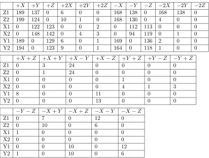
1 Number of configurations able to maneuver into the goal space. Row label indicates
the crystal build pattern. Column label indicates the goal translation. Additional detail and results available in the appendix. . . 33
LIST OF FIGURES
1 The Crystal robotic system(left) and Molecule robotic system(right). Photo from:
http://groups.csail.mit.edu/drl . . . 2
2 The superbot robotic system. Photo from: http://www.isi.edu/robots/superbot.htm 2
3 A view of a portion of the QSAT reduction . . . 9
4 Visual representation of some possible sliding cube moves [1]. . . 11
5 ATRON makeup and motion [2]. . . 13
6 A sequence of images demonstrating ATRON moves. The first frame shows both the
starting and ending positions of the module [3]. . . 13
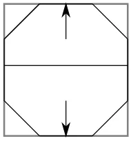
7 A side view of an ATRON module inset inside a cube representation. The arrows
indicate the polar axis, and the center line indicates the “equator”. . . 20
8 Overview of key classes in the simulator . . . 23
9 A sample starting configuration from the new ATRON simulator. . . 26
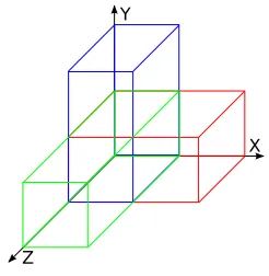
10 A representation of ATRON starting states aligned along the X (red), Y (blue), and
Z (green) axes. . . 26
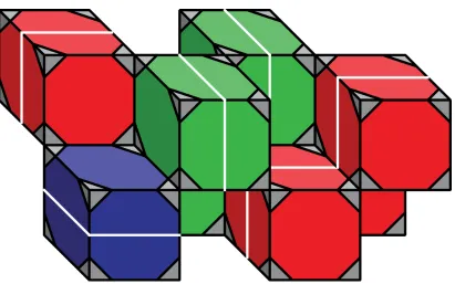
11 An ATRON starting state showing the ATRON traits projected onto the cubes used
in the simulator . . . 27
12 A neighborhood of modules. The arrows indicate the “rotational pole” of the module.
CHAPTER 1
Background
1.1
Self-Reconfiguring Robots
Robots can be found in a very wide variety of shapes and forms. Robotic aircraft provide intelligence
to our soldiers in the field, while robotic sweepers clean our floors. We have designed robots to
explore other planets, and designed experimental robotic systems in a number of different forms.
The vast majority of these robotic forms are static in nature. They cannot change their forms
or capabilities to adapt to new tasks or situations. While a robotic arm might be able to wield
different tools, it would be ineffective at climbing walls. A long legged walking robot would likewise
be a poor choice of tool to navigate a narrow tunnel.
To provide that level of flexibility, a new type of robotic system called a dynamically
reconfig-urable robot [4] or a self-reconfiguring robot has been proposed. In this system, a robot is made up
of a number of smaller robots who function as a team. The shape of the resulting system is highly
variable, allowing the system to configure itself in the fashion best suited to the task and situation
at hand. Systems of this type allow for very complex behavior to be achieved using relatively simple
component structures, much as biological systems derive complex functions from relatively simple
cells. Several different implementations of this general concept have been proposed. Examples
in-clude the SUPERBOT system [5], the ATRON system [6], the Molecule system [7], and the Crystal
Figure 1: The Crystal robotic system(left) and Molecule robotic system(right). Photo from: http://groups.csail.mit.edu/drl
Figure 2: The superbot robotic system. Photo from: http://www.isi.edu/robots/superbot.htm
system [8].
These systems a generally divided into two broad categories: chain-based and lattice-based.
A chain-based system is one in which the individual modules form a whole via connected linear
structures. The kinematics of such a system are necessarily complicated, and they are particularly
suited to particular types of non-reconfiguring locomotion, such as wheels, leaping, crawling, etc.
A lattice-based system is one in which the modules occupy connected locations in a lattice-like
structure. Such systems, including all of the systems above, are very well suited to reconfiguration
in a wide variety of ways. Systems of this type can be either two or three dimensional in their
kinematics.
Self-reconfiguring robots have by definition the ability to reorganize their components to reflect
different shapes or movement characteristics. In systems where modules differ in construct from one
[image:10.612.230.384.252.366.2]poses a series of new computational challenges, however. A simple high-level command such as
“move north” must result in an algorithm determining action (if any) for all the component modules,
instead of simply applying power to the motive system. Of particular interest in this work is an
efficient algorithm for motion planning for the system. In order to move the system, paths must be
determined for all modules composing the system (through an ever-changing environment composed
of their peers). In theory, these systems could be composed of thousands or millions of modules, so
sublinear space and time requirements are extremely desirable algorithm traits for this application.
A further desirable trait of this algorithm is that it should be able to function within
reason-able parameters regardless of the specific kinematic nature of the underlying hardware platform.
As noted above, many different hardware implementations, each with different kinematic natures
already exist. As this technology matures, it is likely that many more platforms will be created.
An algorithm capable of path planning regardless of the hardware specifics would be an extremely
valuable tool for working with this class of equipment. Ideally, such an algorithm could simply be
provided with a goal location or final configuration and would determine the individual module
moves required to achieve it.
1.2
This Work
This work examines the application of Fitch and Butler’s Million Module March algorithm [9] to
the ATRON hardware platform, with implications for the set of all self-reconfiguring robots. The
somewhat chain-like kinematics of the ATRON platform make it very distinct from the SlidingCube
platform, and ATRON has so far resisted attempts to reduce it (via meta-modules) to a SlidingCube
abstraction. Were the Million Module March algorithm to work on the ATRON platform, it would
likely cover a significant portion of the set of all self-reconfiguring robotic kinematics, and it might
be possible to show that it would cover all of them. Unfortunately, in this work we will establish
that this is not the case as the algorithm does not, and cannot, work on with ATRON’s kinematics.
We further establish that any algorithm of sublinear runtime cannot successfully plan ATRON’s
kinematics.
In section 1, we provide background information necessary for this work. We introduce the
concept of Self-Reconfiguring Robots, discuss planning algorithms designed for these systems,
in-troduce the Million Module March algorithm, and inin-troduce the ATRON hardware platform. We
also introduce the concept of a Markov Decision Process, and a Partially-Observable Markov
De-cision Process, and establish a proof demonstrating that a Partially-Observable Markov DeDe-cision
Process is hard for P-Space.
In section 2, we introduce a prior proof of reachability for a two-dimensional system of sliding
squares, and then use this to prove the reachability of a three-dimensional system of SlidingCubes.
We also discuss how this proof provides the theoretical basis for the functioning of the already
proven Million Module March algorithm. We then discuss the differences between the ATRON and
SlidingCube kinematics, and demonstrate how ATRON violates the necessary requirements for the
reachability proof. This violation establishes that ATRON motion planning cannot be phrased as
a local MDP over space, but must return to the default POMDP over the robot (partial as we
restrict ourselves to local knowledge). We also discuss the changes made to the simulator codebase
to perform simulations for the ATRON kinematics.
In section 3, we discuss in greater detail the failure states observed during simulation, and how
ATRON’s reduced mobility affects the convergence of reward values. We discuss how, based on the
increased mobility and reachability guarantees previously discussed, SlidingCube cannot suffer these
failure states. The failure states particularly illustrate the fundamental failure is the insufficiency
of local knowledge to plan ATRON system movement, as opposed to simple state representation
failures or some other implementation detail. Two main failure states were observed, which we
term kinematic orphaning and thrashing. Kinematic orphaning is a result of a module being left
with no meaningful moves to make, and is previously proven to be an impossible occurrance for
SlidingCube. Thrashing results due to the way the algorithm converges reward values, such that
the module in question is surrounded by space for which reward values have not been converged,
which is also an impossibility with SlidingCube’s kinematics. We present the aggregated results of
of the algorithm to plan for the ATRON kinematic platform. We discuss the necessary complexity
of any algorithm capable of correct planning for the ATRON kinematic platform.
1.3
Other Planning Algorithms
The problem of motion planning is essentially the problem of moving a robotic system from its
intial configuration into another space. It is generally considered to be distinct from the problem
of configuration planning, in which a self-reconfiguring robotic system moves from an initial
con-figuration to a final concon-figuration in which individual modules have a defined final position. The
distinction for motion planning is that the goal is generally less tightly defined, the final position
of an individual module generally isn’t considered so long as the system is “over there”.
Butler and Fitch’s proposal of the Million Module March algorithm, on which this work is based,
is discussed at length in the next section. That work was preceded by Butler’s work with Kotay,
Rus and Tomita [10], which laid the groundwork for generic self-reconfiguring robotic systems. In
this work, a generic set of local movement rules for lattice-based robots capable of particular set of
moves is proven. Butler and Rus also proposed a similar algorithm, referred to as Pac-Man [11].
Pac-Man is a parallel algorithm, which runs on a compressible cube kinematic, which is similar
to the SlidingCube abstraction, but unlike Million Module March it plans complete paths to a
completely specified final configuration, giving it linear space and runtime characteristics. This
work, like Fitch and Butler’s previous work, uses only a simple bounding box for the goal space.
Christensen proposed a distributed algorithm for ATRON reconfiguration using meta-modules
[2]. A meta-module is a small collection of modules, which may be treated as a single module
with kinematic traits which make planning easier. Planning for modules within a meta-module
often consist of simple motion rules for how to achieve the desired available motion of the
meta-module. Brandt and Christensen proposed an ATRON meta-module that satisfies the SlidingCube
abstraction in two dimensions, and demonstrated the Million Module March algorithm with it [3].
So far as we are aware, no three dimensional ATRON meta-module satisfying the SlidingCube
abstraction has been proposed. Meta-modules are not examined in this work, so the applicability
of the Million Module March algorithm to ATRON via meta-modules remains an open question.
Stoy and Nagpal proposed a lattice based algorithm that uses multiple bounding boxes to
represent the goal configuration, allowing for configuration specification while still requiring less
space than the size of the robot [12]. Their work uses simple motion rules to guide module motions,
and does not compensate for obstacles.
Varshavskaya, Kaelbling and Rus proposed a reinforcement learning algorithm to distill motion
rules [13]. The algorithm uses an MDP formulation to process learning experiences, and is capable
of being run in a distributed fashion. However, as this system is designed to distill motion rules, it
is not designed to handle changing terrain or unusual obstacles.
Pamecha et al. proposed a method of calculating the distance between two configurations,
and an algorithm for motion planning based on those calculations [14]. This distance calculation
proceeds on the assumption that the kinematically optimal path will correspond to the cartesian
distance between portions of the starting and goal configurations. Further, the algorithm’s runtime
is a polynomial of the number of modules.
1.4
Markov Decision Process
The problem of motion planning for a robotic system has a trait, called the Markov property,
which makes it particularly well suited to being solved with a reinforcement learning technique.
Formally, having the Markov property means that the conditional probability for transition between
states depends only on the current state, not on any previous state. In essence, this means that
the problem can be framed in such a way that the results of future actions can be reasonably
predicted from current state data. Said another way, the only knowledge required to determine the
appropriate action to take is knowledge of the current state, as opposed to historical state data.
This assertion of the Markov property is significant for two reasons. Firstly, by asserting that
all information necessary to determine action is present in the current state, we vastly simplify the
amount of data that must be considered at each time step. Secondly, we can formulate a Markov
An MDP is essentially formulated of a four-tuple,hS, A, T, Ri. S represents the set of all
pos-sible states, A is the set of available actions, T represents the transition function mapping the
combination of starting state and action to resulting state, and R is a reward function. With these
established, formulae have been established to maximize the reward values at a given timestep for
the four-tuple. The existence of these general formulas, which have been proven in the general case
for Markov systems, additionally simplifies the problem of creating an algorithm for this particular
application.
1.5
Partially-Observable Markov Decision Process
By definition, a Markov Decision Process requires that the agent have complete knowledge of the
state of the system (S in the four-tuple). However in some problems this complete knowledge may
be unavailable. In this case the problem becomes a Partially Observable Markov Decision Process,
or POMDP.
A POMDP is, formally, quite similar to an MDP, and utilizes the same four-tuple. However S
and T in the four-tuple represent stochastic distributions across the range of possible states based
on the limited observation of the agent. It has been shown that solving a POMDP is hard for
PSPACE [15]. This represents a significant increase in difficulty over a basic MDP, and indicates
that it is likely infeasible to calculate for large problems, including the motion planning problem
under discussion.
What follows is a proof of the claim that solving a POMDP is hard for PSPACE. Much of this
discussion is taken from [15].
The Quantified Satisfiability problem, or QSAT, is the question of whether a boolean formula
can be true. A quantified boolean formula is of the form ∃x1∀x2∃x3...∀xnF(x1, ..., xn) whereF is
a formula in conjunctive normal form with three literals per clause. The question is whether there
is a set of values that can be assigned to the existential variables, such that regardless of the value
of the universal variables the formula is true. This problem has been shown to be complete for
PSPACE, and it will be demonstrated that solving a POMDP is hard for PSPACE by reducing
QSAT to a POMDP.
In formally phrasing the POMDP, an extra trait will be noted representing the uncertainty in
state signal. States will be grouped into sets, such that the solver is able to determine what set
it is in with certainty, but cannot know which state within the set it is in. Actions are phrased
relative to sets, transitions relative to states. This has the effect of limiting the complexity of the
POMDP, however it is obvious that the full POMDP cannot be less complex than this limitation.
In QSAT there are∃x1∀x2∃x3...∀xnF(x1, ...xn) withnvariables (both existential and universal),
and mclauses C1, ...Cm. In the following notation, variables will be associated with j, and clauses
withi.
S in the POMDP contains s0, which is the initial state, and e0 which is the ending state. S
also contains six states Aij, A0ij, Tij, Tij0, Fij, Fij0 for each clause Ci and variable xj. There are also
2m states Ai,n+1, Ai,n0 +1. The initial state s0 and e0 are each in their own set. For every variable
j, the states Aij, i= 1, ..., m form the set called Aj. Similarly, the states A0ij, i= 1, ..., m form
the set A0j, the states Tij, i= 1, ..., m form the set Tj, the states Tij0, i= 1, ..., m form the set Tj0,
the states Fij, i= 1, ..., m form the set Fj, the states Fij0, i= 1, ..., m form the set Fj0, the states
Ai,n+1, i= 1, ..., mform the setAn+1, and the states A0i,n+1, i= 1, ..., mform the set A0n+1.
Informally, the problem structure is somewhat easier to summarize. The problem space begins
with the first transition from the starting state to the states A0i1. Once this transition has been
made to a particular value of i, the process is locked in states subscripted by i until termination.
Therefore, on any given pass, only a single clause of the original formula is being examined (and
all transitions operate based on a particular clause). Since which clause has been ’selected’ in this
way is hidden, any solution for the POMDP must function for all such clauses. Once the initial
transition has been made, and therefore a clause chosen, there are two groups of states,Ai andA0i.
The goal is to transition into the statesAi prior to termination, because once in that set of states
the only transition out is to the end state, and the only transition to the end state with zero cost
is from that set. We start, as mentioned earlier, in the setA0i. The set of statesT and F represent
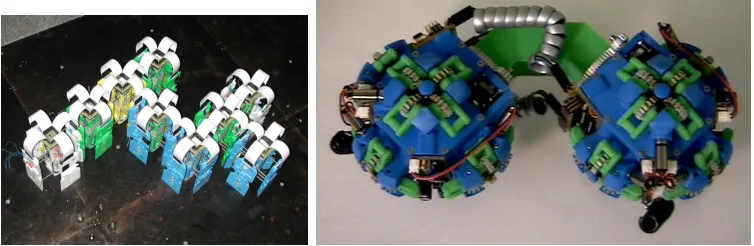
[image:17.612.84.529.69.659.2]
Figure 3: A view of the state space, connections, and rewards of a portion of the QSAT reduction. This shows the connections between the sets of states of a single subscripti, which would be chosen at random transitioning froms0
is via a truth assignment (T or F) which would result in the clause being true. This trick relies
on the equation being expressed in Conjunctive Normal Form, so that any variable may cause the
clause to be true, and once a variable has done so, no further variable assignments may reverse it.
Returning to the formal description, A and T in the POMDP are highly related and so will
be described together. s0 has only one action, which transitions with equal probability to the
states A0i1. If xj is an existential variable, there are two actions in the set Aj, which transition
with certainty from Aij to Tij orFij. In the same case there are two actions in the setA0j, which
transition with certainty fromA0ij toTij0 orFij0 . Ifxj is a universal variable, there is one action in
the setAj which transitions with equal probability fromAij toTij andFij. In this case there is also
one action in the set A0j which transitions with equal probability fromA0ij toTij0 and Fij0. The sets
Tj and Fj each have one action, which transitions with certainty from Tij or Fij (respectively) to
Ai,j+1. Ifxj is positive inCi, then there is one action in the setTj0 which transitions with certainty
fromTij0 toAi,j+1, and one action in the setFj0 which transitions with certainty from Fij0 toA0i,j+1.
If xj is negated in Ci, then there is one action in the set Tj0 which transitions with certainty from
Tij0 toA0i,j+1, and one action in the set Fj0 which transitions with certainty fromFij0 toAi,j+1. The
setsAn+1 and A0n+1 each have one action, which transitions from Ai,n+1 and A0i,n+1, respectively,
toe0 with certainty.
The reward function, R, for this POMDP is quite straightforward. The reward for all transitions
is zero, save the transition fromA0i,n+1 toe0 which has a reward of -1.
It is claimed that a policy with an expected cost of zero exists for the POMDP iff there is an
assignment of variables that results in the formula being true. Suppose the existence of such a
policy. The transition from the initial state can be to any stateA0i1. Once the process has entered
the set A01, it remains in states subscripted by that value of i until the process terminates. The
policy must guarantee that the process proceeds through Ai,n+1, or else the expected cost will be
at least 2−n/m. In order to wind up in Ai,n+1, the process must make decisions for existential
variables corresponding to values which will make the clause Ci true. Since all clauses must be
(a) (b)
Fig. 3. Action space with respect to a given face for a SlidingCube module. The wireframe box is the state (lattice position) in question, grey boxes are adjacent modules. In (a), there are four possible sliding transitions, indicated by arrows, with respect to the bottom face. Rear arrow not shown. Similar convex transition actions are shown in (b). Cases are symmetrical for remaining five faces.
Fig. 4. Graphical representation of a policy in our MDP formulation, with the robot shown in cross-section. Each square represents a state, grey squares are occupied by modules, and the dashed-line box is the goal. Arrows indicate the optimal action to be taken by a module in that state. Straight arrows are sliding transitions, and right-angle arrows are convex transitions. Any module taking the indicated actions follows a shortest path to the goal.
(MDP) and solve it using dynamic programming (DP). This MDP will be stored in a distributed fashion; state updates are computed by adjacent module pairs. Because the DP updates (Bellman backups) execute in parallel, the policy converges in sublinear time in the size of the robot. As modules move, the underlying MDP also changes and we update the policy. Iterating this process, all modules reach the goal region. In practice, this process converges rapidly. The resulting policy yields a path from all open positions in the current configuration to a position in the goal region. It is important to note that the policy does not map modules to actions, or local neighborhood configurations to actions. Instead, the policy maps lattice positions, which are points in space, to actions. A given module may follow a path to the goal by following the optimal action associated with each lattice position it traverses, as depicted in Fig. 4.
A. MDP Formulation
To be more precise, an MDP is a4−tuple < S, A, T, R >, where S is the set of states, A is the set of actions, T is the transition function, andRis the reward function. In our MDP formulation, a states∈S is a lattice position, and an actiona∈Ais a primitive module actuation. The transition function T maps each (s, a) pair to the resulting lattice position s!. T is deterministic and known by all modules.
State-action pairs that result in collision with an obstacle or another module transition to a state with a large negative reward. Otherwise, a reward of -1 is given for each action that does not transition into the goal region. For s! in the goal region, the reward is 0 plus a small negative value determined by the height of the lattice position above the ground, decreasing from 0 towards -1. This reward function results in modules moving first into the goal region and then towards the ground as far as possible. This represents a goal ordering that avoids creating unreachable holes in the goal configuration.
The state space S is essentially that of the gridworld common in the reinforcement learning literature, but in three dimensions. These are world-centered coordinates – as the robot locomotes, its modules move through this state space. At the beginning of a locomotion task, a coordinate frame is attached arbitrarily to the robot. Since they know the transition function, modules can easily maintain their coordinates in this frame subsequently. Although the set of all lattice positions is infinite, the MDP only considers a small finite portion of it: lattice positions occupied by or adjacent to modules in the robot.
The action spaceAis determined by the primitive actions available to a module in a particular state. The total number of actions for a SlidingCube module disregarding symmetry is 48. With respect to a certain neighbor, the possible moves are sliding or convex in each of the four cardinal directions, as seen in Fig. 3. The other faces are symmetric. Therefore we have 8 × 6 = 48 possible actions. Many of these transition to the same destination however, and only a subset are available at any given state. In particular, sliding and convex transition moves are mutually exclusive for a given neighbor and direction. This is determined by what modules are in the local neighborhood. Therefore we may reduce the action space to four actions per neighbor, or equivalently, per face. It is also possible to make no move at all, so the null action is always valid. Our set of actions then is
{fiaj|0< i≤6,0< j≤4} ∪ {do nothing}.
The MDP is formulated as if there were a single module, or agent. We know that in reality we have multiple agents, but a flat representation of their collective state grows exponentially in the number of agents. To overcome this problem, we use a multi-agent abstraction where all agents share the same policy and are assumed to be independent. Of course, agents are in fact dependent on each other in avoiding collisions and preserving global connectivity. We use a separate process to deal with this issue, described in the next section. Furthermore, as modules move, the structure of the MDP changes. This corresponds to barriers changing location in gridworld terms. This is why DP updates are processed continuously in response to module movements. B. MDP Implementation
Since the action-value function is defined over lattice positions, considering only those adjacent to module faces, it is natural to store it within the modules and propagate value updates in a parallel distributed fashion. The policy therefore
ThB7.4
2250
Figure 4: Visual representation of some possible sliding cube moves [1].
In the other direction, if the formula is true, then there must be a policy for setting the existential
variables, based on the values of the universal ones, such that all clauses are satisfied. This is also
a policy for choosing the corresponding decisions at the sets corresponding to existential variables
so that any clauseCi is satisfied, and the state Ai,n+1 is reached. This completes the proof of the
reduction.
1.6
Million Module March
Fitch and Butler proposed an algorithm for locomotion planning for self-reconfiguring robots that
has sublinear time and space requirements [9]. The algorithm uses dynamic programming
tech-niques to solve a Markov Decision Problem formulation of the motion problem. The fully observable
nature of the problem will be discussed in following sections. Exact goal configuration would
obvi-ously require memory linear to the number of modules, so the goal state is simplified by representing
it as a bounding box. This allows the goal to be represented with constant storage, regardless of
the number of modules.
The algorithm was proven to successfully generate navigation, theoretically and experimentally,
for the SlidingCube abstraction. These cubes are capable of moving, without assistance from
neighboring modules, in the direction of any face of the cube. It is also capable of making convex
moves around neighboring modules, as seen in figure 4 (b). This allows each module to plan its
motions independently of the others. It is worth noting that concurrency issues, such as collision
avoidance, are not handled by the planning component of the algorithm expressly, but rather by
simple locking routines at the time of motion. Maintaining connectivity is maintained similarly.
Additionally, it has been shown that this abstraction fits a number of different potential and actual
hardware systems [10].
The algorithm treats the issue of locomotion planning as a Markov Decision Problem (MDP).
S in this MDP is simply the module’s location in space. A is the set of actions available to the
module, and is the set of actions kinematically possible for a SlidingCube given its neighbors. The
reward for a given state is set to -1 for all positions outside the goal area, and a smaller negative
value dependent on height, designed to drive modules to the bottom of the goal. This MDP is
then solved using a dynamic programming technique. Modules each plan reward for adjacent space
based on the reward values that can be reached from those spaces. Spaces that are unreachable due
to the presence of an obstacle or that would cause disconnection from the group are artificially given
a reward of negative infinity, which ensures that any valid move is taken prior to this move. The
algorithm traverses space beginning with the goal space, and traverses the surface of the robotic
system. This approach makes the assumption that any mobile module is capable of maneuvering
across the surface of the robot, which we will demonstrate is true later in this work.
The algorithm is designed such that every module may plan its motion independently of the
others in the robot. Collisions during concurrent motion are avoided by means of announcing a
“lock” on a space when the move is initiated, which causes any module that wished to move to
this position to instead take no move. Moves are planned with only minimal regard to neighbors,
checking to ensure that no disconnections will take place, as the algorithm assumes that each
module’s motions are independent of those of its neighbors. However, the simulator is designed to
run in a single-threaded fashion, so module planning is done one module at a time. State information
is stored in a hashtable, which means that storage space is is only allocated for states that are used
at some point during motion. This also means that the simulator does not explicitly simulate
distributed storage or message passing amongst the modules. However, the implementation of
these aspects would be very closely tied to the hardware capabilities of a specific platform, and do
surrounding. Based on this modules decide when to emerge a meta-module, how it should move and when to stops. The part of the modules’ controller that makes these decisions are three small artificial neural networks (ANN). The ANN’s takes input calculated from the subset of the reachable space of the meta-module. As outputs one ANN gives a decision on whether to emerge. A second ANN gives as output whether to stop. The third ANN assigns a fitness value to every state in the known subset of the reachable space graph. The meta-module will move towards the fittest state. We evolve the weights of the ANN controller by letting the system shape-change and measure its performance as a fitness value.
The combination of ATRON modules, meta-modules, attraction-points and evolved artificial neural network control gives rise to a robot which can change its shape and self-repair in a large range of scenarios. This slightly complex control strategy is the best known solution to the complex problem of shape-changing and self-repairing large structures of ATRON modules.
II. Related Work
Besides the ATRON module, hardware prototypes of modules able to self-reconfigure in 3D include the MTRAN [14], 3D-Unit [13], Molecule [10] and I-Cubes [22]. One main difference between ATRON and these systems is the complexity of the individual module in term of degree of freedom. The ATRON module’s single degree of freedom may make it simple to manufacture but hard to control.
Most prior work, on shape-change of self-reconfigurable robots, focus is on achieving a particular target shape. This is problematic to achieve for systems such as the MTRAN and ATRON, because of difficult motion constraints on the modules. Inspired by Bojinov et al. [3] we avoid this problem by trying to achieve a particular functionality instead of a particular target shape.
Controlling shape-change of large groups of modules makes direct search strategies infeasible because of the computational complexity involved. Planning strategies are often possible on smaller groups of modules, to solve a sub-problem or using heuristic search [10], [21], [24]. Distributed control [4], [5], [11], [16] strategies are indepen-dent of the global properties of the structure of modules. This helps to ensure robustness, but distributed control may be harder to design than centralized control.
In [1], [6], [12], [17], [18], [21], [23] groups of modules are used as meta-modules to handle the base modules’ motion constraints. A negative characteristic of meta-modules is that they increase the granularity of the system. Also the increase in cost and complexity of a single meta-module, compared to a single module, might be difficult to justify with the improved mobility.
Prior work on self-repair in self-reconfigurable robots generally involves the detection of module failure, decisions on how to remove a defect module and how to replace it with a spare module [7], [20]. Alternatively, as in this work,
Fig. 2. Photographs of: (a) A single ATRON module, on the top hemisphere the two male connectors are extended on the bottom hemisphere they are contracted. (b) A structure of seven ATRON modules connected in the surface-centered cubic lattice structure.
self-repair can emerge as a side effect of the control instead of having a specialized self-repairing part of the controller [19].
Artificial evolution has previously been used on self-reconfigurable robots to automate the design of control. Østergaard et al. [15] evolved with limited success dis-tributed state-machine based controllers for small struc-tures of 12 to 20 ATRON modules. Similarly evolution was used on small groups of MTRAN modules to automatically generate locomotion patterns [9]. For the 2D metamorphic system genetic programming was used to generate con-trollers for movement of 8 modules to solve tasks such as moving through a narrow passage [2].
III. The ATRON Self-Reconfigurable Robot The ATRON module, has a single rotational degree of freedom and is able to self-reconfigure in 3D, see figure 2(a). It has a spherical appearance composed of two hemispheres, which the module can actively rotate relative to each other. The modules connect to neighbour modules using its four actuated male and four passive female connectors. The connectors are positioned in 90 degrees intervals on each hemisphere. Using infrared channels the module is able to communicate with neighbour modules and sense distance to nearby obstacles or modules. Two ”Atmel ATmega128” microcontrollers, one on each hemi-sphere, controls the module. A module weighs 0.850kg and has a diameter of 110mm. 100 hardware prototypes of the ATRON modules exist. A more extensive description of the ATRON hardware can be found in [8]. In this work the modules are always connected in a surface-centred cubic lattice structure, see figure 2(b).
Motion constraints on the modules affect their ability to self-reconfigure. The single rotational degree of freedom of a module makes its ability to move very limited, in fact the module morphology does not allow it to move by itself. One module may move another module by rotating it while
[image:21.612.249.365.75.184.2]2540
Figure 5: ATRON makeup and motion [2].
Figure 6: A sequence of images demonstrating ATRON moves. The first frame shows both the starting and ending positions of the module [3].
The independent planning capability of the algorithm is the second key to its sublinear running
time. MDPs have been shown to be complete for P [15]. This means that were the state of the
robot as a whole to be needed to converge a path for a single module, the algorithm would not be
able to even approach the desired space and time bounds. However in this case the runtime of the
MDP for a module is a function of the distance between the module and the goalspace.
This algorithm has been experimentally confirmed to operate using the SRSim simulator. [1]
This software simulates a robot composed of sliding cubes.
The simulation experiments not only confirmed the algorithm’s sublinear running time, which
allows it to serve as a control mechanism for a robot composed of a previously unfeasible number
of modules, but also showed the algorithm’s capability to deal with terrain obstacles in an efficient
manner.
1.7
ATRON
ATRON is a homogeneous, modular self-reconfiguring robotic system developed at the University
of Southern Denmark [6]. The design goals of this system were inspired by two existing
self-reconfiguring robotic platforms, CONRO and M-TRAN. Both of these systems reconfigure modules
relative to neighbors based on rotational motion, as does ATRON.
An ATRON module 5 consists of two identical hemispheres, joined together with an innovative
slip ring. This construct allows the hemispheres to rotate infinitely relative to each other, while
still permitting power and communication to flow between them. Each hemisphere also has four
mechanical mating surfaces, which can be used to connect to neighbor modules. Two of these
surfaces are “male”, two “female”. The modules are designed to permit communication along
these mounting surfaces, which allows for the use of distributed algorithms such as the one under
CHAPTER 2
Work Performed
2.1
Formulating SlidingCube as a MDP
Based on the descriptions provided in section 1.5, it would appear at first glance that framing the
SlidingCube motion planning problem based on its Markov property would result in a
Partially-Observable Markov Decision Problem. The complete state of the robot and environmental obstacles
are occluded to individual modules, and therefore cannot be taken into account in the MDP
eval-uation. Additionally, an MDP operating over the state of the entire robot cannot have a sublinear
runtime relative to the size of the robot. However, it turns out that the kinematics of a SlidingCube
module allow the MDP to be formulated in a very different way, which greatly reduces the problem
scope.
In this discussion, a sliding square is a two dimensional module that has the kinematic
capabil-ities of a SlidingCube in two dimensions. Dumitrescu and Pach demonstrated that the kinematics
of sliding squares in two dimensions have the property that any two connected configurations
hav-ing the same number of modules are guaranteed to be able to reconfigure into each other, in the
absence of obstacles [16]. The proof of this consists of an algorithm proving that any arbitrary
configuration may be reconfigured into a straight horizontal line of modules located at the highest
X-axis value; the obvious corollary is that the straight line of modules may be reconfigured into
any arbitrary configuration by reversing the steps of the algorithm. An overview of the algorithm
follows, and the reader is directed to [16] for a complete proof of this trait.
2.1.1 Sliding Square Reachability Algorithm
Consider an arbitrary connected arrangement of sliding squares. The arrangement will have an
outer border, and the interior will contain zero or more holes (entirely contained spaces). The
borders of these holes will be referred to as inner borders. The entire configuration may be
rep-resented as a connected graph with modules as the vertices, and connections between modules as
edges. This model provides a convenient vocabulary for describing the steps that follow. The set
of modules that have already joined the horizontal line (and will thus no longer need to move) is
referred to as Z.
Step 1: If there is a vertex of degree one which is not part of Z, perform this step. Otherwise,
proceed to Step 2.
Step 1A: If there is a vertex of degree one in the outer border, it may be moved without
disconnection to the next open position in the horizontal line, thus joining Z. Following this, return
to the beginning.
Step 1B: If there is a vertex of degree one which is not on the inner border, it may be moved
without disconnection to a position where it is of degree at least two. This is guaranteed by its
position as being an inner border (there must exist a “corner”). Following this, return to the
beginnning.
Step 2: In reaching this step, we are assured that all squares not in Z are of degree of at least
two. In this case, we are assured that there is a maximal cycle with a single connector (see [16] for
the full proof of this statement). The selected vertex should be part of one of the vertical edges
of the cycle which does not contain the singular connector. Since the selected module is not the
connector of the cycle, it may be removed without disconnecting the graph.
Step 2A: If the selected vertex is part of the outer border, it may be moved to the next open
Step 2B: If the selected vertex is not part of the outer border, then move it within its space
such that it is no longer part of the cycle. This obviously does not disconnect the configuration.
2.1.2 Three Dimensional Algorithm
The reachability principal proven in two dimensions also carries into three dimensional figures. We
will now demonstrate an algorithm which will convert an arbitrary three dimensional connected
configuration of SlidingCubes into a fixed configuration, namely a straight line extending along the
direction of the X axis. It can be seen that proving this algorithm is sufficient to prove any two
arbitrary configurations of the same number of modules may be converted into each other.
For convenience, we will refer to the set of modules that are already in the final configuration
as D. A space which is completely bounded by modules is referred to as a hole. A space which is
partially bounded by modules is not given a particular name. It is noted that when such a space is
contiguous with the space outside of the configuration, the bordering modules are part of the outer
border of the configuration. For the purposes of this discussion two modules are considered to be
neighbors if they share a face, but not if they only share an edge or a corner. A module (or space)
is considered bounded if all six faces have neighbors. The presence or absence of modules on the
corners or edges does not impact on the bounding.
Step 1: Select the module with the highest X-coordinate. If multiple modules have the same
maximal X-coordinate, then one of these may be selected at random. The selected module will be
referred to as m. We will utilize a tree to represent the configuration. To create the tree, we will
utilize a queue, initially populated withm. So long as the queue is not empty, we will remove the
first item from the queue, insert any connected modules that are not already present in the tree into
the tree as its children, and insert those same modules into the queue. Modulem is then declared
to be in its position in D, without moving. An important trait of the tree we have created is that
all leaves on the tree are mobile, which is to say that they may be moved without disconnecting
the configuration. In this context, mobile does not imply that the module is kinematically capable
of moving, it may be blocked in place by other modules. Another important trait of the tree as
we have constructed it results from m having been selected as having a maximal X-coordinate.
This means that of its neighbors, only one can possibly not be on the outer border, which further
means that there can only be a single chain from leaf to root that does not contain a module on
the outer border. Such a chain, if it exists, can only exist so long as there are other chains, which
by definition must contain modules along the outer border.
Step 2: If there is a leaf which is on the outer border, then move it to the next position in D and
remove it from the tree. By definition such a module is mobile, and kinematically free to move. It
may be observed that the SlidingCube kinematics are sufficient for a module to traverse the outer
border to any other position on that border. If after completing this step there is another leaf on
the outer border, repeat this step. If there is no such leaf, proceed to step 3.
Step 3: Select a leaf at random. If none of the leaf’s ancestors (except the root) is on the outer
border, select another leaf. Note that the tree traits guarantee that there must exist a leaf with an
ancestor (other than the root) which is on the outer border. The ancestor which is on the outer
border will be referred to as n. If any child of nis on the outer border, select it as n. Select a leaf
child of n, which we will refer to as o. Since o is not part of the outer border, o has access to at
least six other modules. Ifois free to move then it has access (by moving) to a greater number of
modules. This means that ohas at least five other modules that it may select as ancestors. If ois
free to move, then it will have more modules that it may move and select as ancestors (in this case,
oin in an inner hole). If any of the available modules is not a child of n, then shiftoto be a child
of that module. Repeat with a new oso long as nhas children. When nhas no more children, it
is a leaf, and may be moved into Q. Note that because n was on the outer border, and shared a
connection with its children, at least one of its children is now on the outer border. Return to Step
2.
By following these three steps, the arbitrary configuration is decomposed to a defined
2.1.3 Implications
The guarantee of reachability for the SlidingCube has several sequential implications for the use
of an MDP to solve SlidingCube module motion planning problem. The first implication is that
so long as the goal space touches the starting configuration, and is sufficiently large to admit all
modules in the robot, the existence of a sequence of moves which will maneuver the modules into
the goal space is guaranteed. This removes the need for any sort of validation step.
The second implication is that there is no move that can be made which will prevent the modules
from being able to be maneuvered into the goalspace, so long as the robot remains connected.
Since preventing disconnection can be accomplished with a computationally simple local search,
this caveat does not increase the size of the problem space. Since optimality is not guaranteed with
the Million Module March algorithm, this means we may safely calculate for only a single timestep.
Optimizing the path behavior would significantly increase the problem scope since time would need
to be considered, as moves could be made that deviate from the set of optimal moves.
The third implication is that every module may be safely planned independently of the others.
Since as long as the robot remains connected, there is no neighbor move that may be made which
will prevent the robot from entering the goalspace, we may safely plan every module considering
our neighbors to be obstacles. Framed this way, the MDP is framed not over the configuration of
the robot, but over the space between the module planning its move and the goalspace. It should
be noted that although the MDP is being converged over space, the space examined is being guided
by the shape of the robot, which further reduces the complexity of the problem. This advantage
would also disappear if the algorithm were to attempt to determine the set of optimal moves.
2.2
Differences Between ATRON and SlidingCube
As previously mentioned, ATRON is a modular self-reconfiguring robot system [6]. Like the sliding
cubes in the SRSim simulator, the modules in the ATRON system form lattice based structures.
However, the design of the ATRON module means that the kinematics and lattice structure differ
Figure 7: A side view of an ATRON module inset inside a cube representation. The arrows indicate the polar axis, and the center line indicates the “equator”.
significantly from the sliding cube abstraction.
The ATRON module can be visualized as two truncated cones joined together at their bases.
The actual shape of ATRONs hemispheres is closer to a four sided pyramid, terminated about
halfway up. ATRON has a connector on each of the pyramid faces, and is capable of rotating
round its main equator. As a result, a single ATRON module is incapable of changing position in
the lattice without external assistance.
The difference in connector locations (and number) from the sliding cube module dictates a
change in lattice structure. If an ATRON module was visualized as a cube, then it would connect
along its upper and lower edges, rather than its faces. The resulting lattice is therefore less tightly
packed than a cubic lattice, as there would be empty spaces adjacent to each “face”. A two
dimensional view of this can be seen in Figure 7. Note that the diagonal edges of the ATRON
module, which are its mating surfaces, occur at corners of the square, which would correspond to
edges in a three dimensional figure.
Similarly, the locomotion kinematics for the ATRON module differ from the sliding cube
kine-matics. ATRON modules must be moved by a rotation from a connected neighbor. If the modules
are visualized as cubes, as before, then the target cube may only move to an adjacent edge on a
selected neighbor. Although a given module is dependent on its neighbors to actually generate
mo-tion, path planning may still be performed by individual modules, although if two modules require
use of the same neighbor this creates an additional planning conflict in need of resolution. This is
the motion.
However, this dependence on neighbor motion is a critical difference from the kinematics of the
Sliding Cube. The biggest fundamental difference is that the guaranteed reachability (see 2.1.2)
between configurations is untrue. The counter proof is quite simple. Given that ATRON modules
cannot generate their own motion, a robot composed only of modules with poles oriented along the
Z axis will only be able to move modules along the X and Y axes, and will not be able to translate
its configuration along the Z axis. Although not within the bounds of our problem, it is also true
that since no move is possible which will change the orientation of any module in that scenario,
it will be unable to assume any configuration calling for a module to be oriented along an X or Y
axis.
2.3
ATRON Implementation
The simulation work builds upon the SRSim program previously created by Fitch and Butler and
used to experiment their algorithm. As previously mentioned, this simulator is built to simulate
a robot consisting of sliding cubes. Therefore, the simulator needed to be adjusted to reflect the
lattice and kinematics of the ATRON system. The nature of these changes was discussed in the
previous section.
In a formal description, the MDP formulation is highly similar to the formulation used in the
original works. It remains a four-tuple hS, A, T, Ri, where S is the state space, A is the set of
actions, T is the transition function, and R the reward function. The individual values within the
tuple have been changed, however. The state space has been modified as discussed above. The
action space is actually restricted from the original work, as for any state and neighbor, only two
actions are possible, as opposed to four in the original work. The transition function is adapted
slightly to accommodate the changed state space, and similarly the reward function is adapted to
reflect a different priority within the goal space.
In the original work, state for the MDP was simply a location. The transition function accounts
for collisions with obstacles or other modules by assigning extremely large negative rewards to these
kinds of moves.
ATRON modules, however, have additional state information and movement constraints over
sliding cubes. Because ATRON modules rely on their neighbors for motion, state must include
connections to neighboring modules. In addition to the previously mentioned situations, high
negative rewards must be assigned to state transitions that are impossible (rotating in nonexistent
ways, for example), and transitions that require use of a neighbor that is already performing another
transition.
Formally, in the original work S was a grid location (x,y,z). In dealing with ATRON, S has
additional variables, becoming (x,y,z,a,s) where a is an axis of orientation for the module, and s is
one (or possibly more) variables representing the state of neighboring modules. In the original work,
the only constraint on T for a given state was whether or not the result was occupied (disconnection
was not handled by the MDP code). In ATRON, T depends heavily on what neighbors are present,
and what their orientations are, so additional neighbor data must be present at some point during
the convergence. Said more simply, having two states (x,y,z,a) is insufficient information to answer
the question of whether there is a transition from one to the other.
While the actual moves available to a SlidingCube do depend on its environment (for example, a
convex move on top of an object requires an object to move on top of), this dependence is different
from ATRON’s dependence. In SlidingCube, a convex move is available regardless of whether
space is occupied by a neighboring module, or simply an environmental obstacle (such as a rock).
ATRON requires actual neighboring modules (obstacles merely prevent motion into the space that
they occupy), and the moves available depend not only on the neighboring modules available, but
also the state (orientation) of those neighbors.
These additional constraints necessarily complicate motion planning for the group, and create
subtle changes in how the algorithm will move the group. Changes to the reward function for
non-goal states necessitated removing a shortcut that stopped converging reward values for a space
if reward values in a connected state did not change. This was not a change to the theoretical base,
needlessly reconverging values that cannot change, but those values can change based on neighbor
movements with ATRON’s kinematics.
2.4
Simulator Codebase
2.4.1 Codebase Architecture
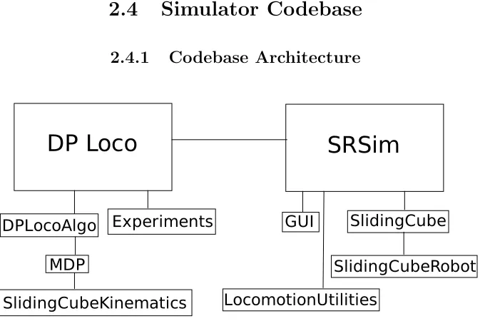
[image:31.612.141.481.139.364.2]
Figure 8: Overview of key classes in the simulator
The SlidingCube simulator, created to perform the Million Module March algorithm, was
writ-ten in Java. The classes of the program are organized into two packages: DPLoco and SRSim.
SRSim primarily contains GUI classes and DPLoco primarily contains the simulator algorithms,
however there are some unusual bindings and divisions of labor between these packages.
In addition to the GUI menus, controls, and displaying the system, the SRSim package contains
the code for the “universe” functions. This includes tracking object location, detecting collisions,
and performing module moves (as distinct from planning). The class “LocomotionUtilities” contains
the methods which perform module moves, and other related utility methods. The package also
contains the classes which are used to represent individual modules and the robotic system (both
in state representation as well as display).
The DPLoco package contains the initial entry point. The “Experiments” class sets up the
specifics of the simulation, any obstacles present, the initial robot size, and how the goal space
moves or changes size. For some simulation cases, the goal may be moved multiple times, with
robot moves in between. The Experiments class therefore also invokes, steps, and/or pauses the
motion planner. The “DPLocoAlgo” class contains the main motion planning algorithm. It does
not contain the actual MDP code which is in the MDP class, but it contains the setup and final move
selection code. The “SlidingCubeKinematics” class contains additional kinematic utility methods
used in motion planning and reward convergence. The MDP and DPLocoAlgo classes also rely
on some utilities found in the LocomotionUtilities class, as well as data stored in the SlidingCube
objects themselves.
2.4.2 Codebase Changes
In order to conduct simulation experiments with the ATRON kinematics, it was necessary to
make significant changes to the simulator codebase. The first changes made were to the section
of code which handled reward values and motion in the goal space. In the original simulator, this
section of code was based around the tendency of the simulator to favor entering the goalspace
from the positive Y direction, and contained a hack to stop motion inside the goalspace. This was
replaced with code which operates in a more general fashion. The revisions were tested against
the SlidingCube kinematics to ensure that it continued to operate in a fashion consistent with the
original works.
Significant changes were also made to the sections of code representing a robot module (both
in data and in display), initializing the overall environment, the kinematic utility functions, and
the MDP code itself. The changes to the robot module and environment code are conceptually
quite straightforward, as they change the initial starting states to reflect ATRON’s axial nature,
and add the data concept of an axial alignment to the module, as well as a display representation
of it. The kinematic utility functions were likewise updated to reflect ATRON’s move types and
neighbor relationships (with axial dependencies). The decision was made for simplicity to continue
displaying individual modules as cube shapes. Kinematically, however, neighbor relationships occur
on edges as opposed to faces, and which edges may be neighbors depend on the axial alignment
changing assumptions, as the original codebase cycled through a static number of faces for each
module, and converged values assuming both a translation and convex move possibility for each
face.
One notable change which was not made to the MDP was the adjustment to explicitly include
axis in the stored reward values. This means that the reward calculated by the code is not for
a true state, but rather the set of states sharing the same X, Y, and Z coordinates. This was
an intentional omission, as the original intent was to develop a kinematically agnostic codebase,
which would be capable of planning a robotic system knowing very minimal information about
the kinematic capabilities of the actual hardware. However, even simulations for ATRON-like
kinematics (for example, a kinematic system where neighbor relations occur on edges, but without
axial alignments) failed to successfully enter the goalspace. Although it is theoretically possible that
the combination of states could result in a planning misstep, none of the failure states examined in
detail exhibited this trait.
In addition to the kinematic and systemic changes required to accommodate simulation of the
ATRON hardware, new features were added to the simulator to allow more interactive investigation
of the model’s convergence, and automate the running of experiments. A new utility was created
which calculated every possible configuration of a given size of ATRON robotic system (assuming a
rectangular prism as a starting shape) and would perform a given experiment on them.
Function-ality was also added to the simulation environment to allow moving forward only a single timestep,
and to report the available moves and associated rewards for a given module (with highlighting in
the display to provide a visual cue for the module being investigated).
2.5
ATRON Starting States
For simplicity, the graphics from the original simulator were largely unchanged. Space occupied by
an ATRON module was represented as a cube, as it had been before. Different colors were used to
represent the different ATRON module orientations, to provide an easier visual representation of
the actual robotic construct being simulated.
Figure 9: A sample starting configuration from the new ATRON simulator.
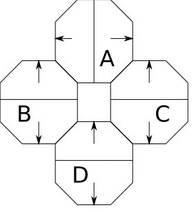
Figure 10: A representation of ATRON starting states aligned along the X (red), Y (blue), and Z (green) axes.
Unlike the sliding cubes, the cubic ATRON representation does not have connections on cube
faces, instead it connects along cube edges. This means that the space occupied will necessarily be
less dense for ATRON when compared to the SlidingCube, since the modules must be offset from
one another in order to actually be connected. For simplicity, crystal structures were composed
of the same number of modules as a SlidingCube cubic crystal, although the resulting ATRON
crystal is actually a rectangular prism. There are three axes which may form the long edge of the
prism (X, Y, and Z). In these prisms, individual layers along the long axis are one of two different
repeating forms. Each form has a void in the location of a module of the other, and a module in
the location of a void of the other, much like the squares of a checkerboard. This means that there
are two different ways to form the prism, depending on which form pattern is the first at the edge
of the prism. There are a total of six total prisms that may be formed for the ATRON module. In
later tables and figures, these prisms are denoted by a letter indicating the axis of the long edge
[image:34.612.244.367.219.345.2]Figure 11: An ATRON starting state showing the ATRON traits projected onto the cubes used in the simulator
arbitrarily assigned, the notation is consistent in form.
CHAPTER 3
Results
3.1
Failure States
The original experimental plan had been to repeat the experiments conducted in the Million Module
March paper [9, 1]. Unfortunately, failure states became apparent that were not addressable by
tweaking constants within the algorithm, such as the default reward values or the learning constant
for the dynamic programming formula. These failure states led to a change in the experimental plan
and data recording, which are discussed in further detail in the next section. It should be noted that
the results here and in the next section are the results of motion planning by the Million Module
March algorithm, and not necessarily reflective of the actual kinematic capabilities of the ATRON
platform. It seems likely that adding some additional complexity to the planning state-space (such
as the axis trait, discussed above) would likely yield more satisfactory results. Other, even more
complex algorithms may be able to successfully navigate all ATRON configurations kinematically
capable of entering the space; however such algorithms are beyond the scope of this work.
The failure modes discussed in this section are a result of some of the fundamental kinematic
differences between the SlidingCube and the ATRON platforms. As discussed in 2.1.3, SlidingCube
has a kinematic reachability guaranteeing that any two connected states consisting of the same
that for SlidingCube, kinematic and physical connectivity are equivalent. In other words, if two
SlidingCube modules are connected physically (either directly or by some number of intermediate
modules), then there exists a series of kinematic transformations, possibly involving other modules,
which will allow them to become neighbors. The ATRON platform lacks this trait, does not have
a reachability guarantee, and therefore kinematic and physical connectivity are different concepts.
This is important because physical connectivity is straightforward to ensure, generally requiring
only an examination of the local neighborhood, and requiring a brute force search in the worst case.
Kinematic connectivity on the ATRON platform is fairly difficult to determine, since a physical
move may have implications for modules far away from the local neighborhood. This difference
between kinematic and physical connectivity gives rise to the two failure modes observed in this
work.
3.1.1 Kinematic Orphaning
The first failure mode is kinematic orphaning. This failure mode can have two different
appear-ances, the first of which is a module chain. This situation occurs when, during transit, a module
cannot move to a position where it would have another neighbor. The chain appearance forms by
maintaining connectivity with the “orphaned” module. This situation arises because the MDP does
not involve path locking, nor does it consider utilizing modules to “help” other modules achieve
the common goal. A fundamental assumption of the algorithm is that if a module is connected
to the main robot, then a path exists for it to move along the main robot surface. The ATRON
kinematics violate this assumption, which leads to the possibility of this failure state. If a module
winds up in a situation where it is connected to only one other module, and no rotation available to
it will bring it into contact with another neighbor, that module is stuck. The algorithm will ensure
that the robot does not become disconnected, but in the process it will leave a chain of modules
from the main robot body to the stuck module. The entire chain, once created, will be unable to
collapse back into the main body using only locally planned motions.
A related failure mode is a module orbiting a finite space, in which it may move to new neighbors,
but only in a kinematically closed loop. Although this does not have the chain’s shape, it is caused
by the same algorithmic traits, and arises from the same kinematic assumptions.
This situation cannot arise with the SlidingCube
![Fig. 3. Action space with respect to a given face for a SlidingCube module.configuration.Figure 4: Visual representation of some possible sliding cube moves [1].The wireframe box is the state (lattice position) in question, grey boxesare adjacent modules](https://thumb-us.123doks.com/thumbv2/123dok_us/51695.4720/19.612.207.407.76.187/slidingcube-conguration-representation-possible-wireframe-question-boxesare-adjacent.webp)
![Figure 5:Fig. 2. ATRON makeup and motion [2].](https://thumb-us.123doks.com/thumbv2/123dok_us/51695.4720/21.612.249.365.75.184/figure-fig-atron-makeup-and-motion.webp)