Verifiable Control of a Swarm of Unmanned Aerial
Vehicles
D. J. Bennet and C. R. McInnes Department of Mechanical Engineering
University of Strathclyde
Glasgow, UK
ABSTRACT
This paper considers the distributed control of a swarm of unmanned aerial
vehicles investigating autonomous pattern formation and reconfigurability. A
behaviour-based approach to formation control is considered with a velocity
field control algorithm developed through bifurcating potential fields. This new
approach extends previous research into pattern formation using potential field
theory by considering the use of bifurcation theory as a means of reconfiguring
a swarm pattern through a free parameter change. The advantage of this kind
of system is that it is extremely robust to individual failures, is scalable and also
flexible. The potential field consists of a steering and repulsive term with the
bifurcation of the steering potential resulting in a change of the swarm pattern.
The repulsive potential ensures collision avoidance and an equally spaced final
formation. The stability of the system is demonstrated to ensure that desired
behaviours always occur, assuming that at large separation distances the
repul-sive potential can be neglected through a scale separation that exists between
the steering and repulsive potential. The control laws developed are applied
to a formation of 10 unmanned aerial vehicles using a velocity field tracking
approach, where it is shown numerically that desired patterns can be formed
NOMENCLATURE
N number of UAVs in formation
U artificial potential field
US steering potential
UR repulsive potential
µ bifurcation parameter
Cr,Lr repulsive potential amplitude and length scale x UAV position vector
v UAV velocity vector
α amplitude of dissipative term
J Jacobian
L Lyapunov function
V UAV speed (m/s) ˙
V UAV acceleration (m/s2)
ψ UAV heading angle (radians) ˙
ψ UAV turn rate (radians/s)
λv, λψ speed and heading angle inverse time constants
Zr repulsive potential sensing radius
g gravitational constant, 9.81ms−2
uc desired cruise speed of UAV, 2.7ms−1
t time (s)
1
INTRODUCTION
Interest in unmanned aerial vehicles (UAVs) has grown in recent years, with a
variety of civil and military applications such as scientific data gathering,
mili-tary reconnaissance and convoy protection [1, 2, 3, 4, 5, 6]. In addition to the
UAVs flying in formation will allow for applications, such as interferometric
imaging, that could not be achieved through single UAVs [7]. As the number of
UAVs increase, controlling the system in a centralised way becomes unrealistic,
so that decentralised control methods have been developed to overcome this
problem.
In the area of distributed multi-vehicle systems some work is motivated by the
emergent and self-organised behaviour that is seen in nature. Through simple
local interactions a school of fish or flock of birds, for example, will aggregate
to-gether to form global emergent behaviour [7]. Brooks [8] introduced the concept
of a behavioural control architecture taking inspiration from natural behaviours.
By having this form of control we can have a system that, although controlled
through relatively simple laws, will achieve a desired behaviour and have the
advantages of being a scalable, robust and flexible system [9].
Artificial potential fields are an example of behavioural control architecture
[7, 10, 11] and were first introduced by Khatib [12] in the area of obstacle
avoid-ance for manipulators. More recently they have been applied successfully in
the area of autonomous robot motion planning [13, 14] and in space
applica-tions [15, 16, 17]. The basic idea behind artificial potential fields is to create a
workspace where each UAV is attracted towards a goal state with a repulsive
potential ensuring collide avoidance [14]. As the UAV swarm may be required
to achieve different tasks, a desirable property of the system would be
reconfig-urability. In order to minimise computational expense bifurcation theory can
be used to reconfigure the formation through a simple free parameter change.
Other approaches to the control of UAVs include Reynolds flocking theory [?]
that takes a set of rules and applies them to all the vehicles in the group.
agents and several authors have since extended his theory and applied it
specif-ically to control a swarm of UAVs [18, 19]. Another approach to UAV control
is graph theory that represents the local interactions and spatial distribution of
a swarm of UAVs in a directed graph [20]. The virtual structure approach is
also used that treats each UAV as a particle that attempts to maintain a fixed
geometric relationship [7, 21].
The purpose of this paper is to investigate the distributed control of pattern
formation and reconfigurability in a swarm of UAVs. A behavioural control
architecture is developed through the artificial potential field method and
bifur-cation theory that allows for the creation of autonomous swarm patterns that
can be altered through manipulation of the free parameters of the potential field.
This new approach consists of a steering and repulsive potential field with the
bifurcation of the steering potential resulting in the formation of different
pat-terns. The repulsive potential ensures collision avoidance and an equally spaced
final formation. The advantages of this system are that it is robust, scalable
and flexible. In addition, for real safety critical applications it is essential that
the stability of the system is ensured. As opposed to algorithm validation this
paper mathematically proves the stability of the system. It is shown that there
exists a scale separation between the steering and repulsive potential so that
UAV system moves under the influence of a far field steering potential but with
short range collisions. It can then be proven analytically that the desired
be-haviours always occur. The model is then applied to a velocity field tracking
approach that generates a set of commands to control the UAV heading and
speed.
The paper proceeds as follows. Insection 2 we describe the model used and
explain the artificial potential field method and bifurcation theory. We also
shows the numerical results of simulations demonstrating pattern formations
and reconfigurability. Insection 4 we consider a swarm of 10 UAVs desired to
form a double ring pattern and then bifurcate into two different ring patterns,
traveling at constant speed and ensuring collision avoidance throughout the
simulation.
2
FORMATION MODEL
2.1
ModelWe consider a swarm of homogeneous UAVs (1≤i≤N) described through a second-order dynamical system as shown in Eq. 1 and 2. The negative gradient
of an artificial potential function, U, describes a virtual force acting on each UAV with mass,m, position,xi, and velocity,vi;
dxi
dt =vi (1)
dvi
dt =−∇iU
S(xi)
− ∇iUR(xij)−σvi (2) It can be seen from Eq. 2 that the virtual force experienced by each UAV is
dependent upon two artificial potential functions and a dissipative term, where
σcontrols the amplitude of this dissipation. The first term in Eq. 2 is defined as thesteering potential, US, and is used to command each UAV to a desired position with the repulsive potential, UR, ensuring collision avoidance and an equally spaced formation.
Therepulsive potential is a simple pairwise exponential function that is based
on a generalized Morse potential [22] as shown in Eq. 3;
UijR=
X
j,j6=i
whereCrandLrrepresent the amplitude and length-scale of repulsive potential respectively and|xij|=|xi−xj|.
The total repulsive force on theith UAV is dependent upon the position of all the other (N−1) UAVs in the formation. The repulsive potential is therefore used to ensure that as the UAVs are steered towards the goal state they do not
collide with each other. Once all the UAVs have been driven to the desired
equi-librium state the repulsive potential also ensures that they are equally spaced
for symmetric formations.
2.2
Artificial Potential Function Scale Separation
As noted in the previous section the dynamics of each UAV is dependent upon
the gradient of two different artificial potential functions. The steering and
repulsive potential are a function of position only with length scaleR andLr respectively as shown in Eq. 4 and 5;
US = f(X, R) (4)
UR=Crexp−X/Lr (5) For illustration we consider a simple 1-dimensional system with position
coor-dinateX.
Defining an outer region dependent upon the steering potential only and an
in-ner region dependent upon the repulsive potential only we can show that these
two regions are separated so that each UAV moves under the influence of the
to determine the non-linear stability properties of the system considering the
steering potential only.
For 1D motion of a UAV of massmand damping constantσwe have;
mdV
dt = − dUR
∂X − dUS
dX −σV (6)
so that,
mV dV dX =
Cr
Lr
exp−X/Lr−dU
S
dX −σV (7)
ScalingX such thatS=X/Rthen;
1
RmV dV dS =
Cr
Lr exp
−R
Lr
S
−R1 dU S
dS −σV (8)
Now defineε= Lr
R <<1 so that;
mVdV dS =
Cr
ε exp
−S
ε −dU
S
dS −σRV (9)
Let ε → 0 in order to consider ‘far field’ dynamics which forms a singularly perturbed system;
lim ε→0 1
εexp
(−S/ε)= 0 (10)
Therefore at large separation distances the repulsive potential vanishes and we
can consider the steering potential only when considering the stability of
anal-ysis of the system.
Conversely if we defineS =S
ε we find that the ‘near field’ dynamics are defined
mVdV
dS = Crexp
−S−εR
1
Lr
dUS
dS +σV
(11)
and lettingε→0;
mVdV
dS =Crexp
−S (12)
Thus, at small separations the steering potential vanishes. If we then consider
the 2nd order system and assume that m/σ << 1 so that the dynamics are overdamped, we obtain a velocity field defined as shown in Eq. 15.
m σV
dV dS =−
1
σ∇iU
S(X)
−1σ∇iUR(X)−V (13) assuming thatm/σ <<1 so that the system is overdamped we find that,
−σ1∇iUS(X)−σ1∇iUR(X)−V = 0 (14) thus,
dX dt =−
1
σ∇iU
S(X)
−σ1∇iUR(X) (15) Each UAV therefore acts under the influence of a long range steering potential
but with short range collisions, allowing us to treat the collisions separate in
the subsequent stability analysis. We can also now use the first-order velocity
field to control the formation of UAVs as shown in Eq. 16;
dxi
dt =−∇iU
S(xi)
− ∇iUR(xij) (16) By assuming that the second-order system is overdamped the UAVs will closely
2.3
Steering Potential - 1 parameter static bifurcation
Referring to Eq. 16 we can base thesteering potentialon asupercritical pitchfork
bifurcation [23] as shown in the first two terms of Eq. 17. This potential drives
each UAV to a goal distance,r, from the origin in thex−y plane with the last term in Eq. 17 ensuring that the formation is created in thex−yplane, where
αcontrols the amplitude of this quadratic potential;
US(xi;µ, α) = −12µ(ρi−r)2+ 1
4(ρi−r) 4
+αzi2 (17) where cylindrical polar coordinates, xi = (ρi, zi)T, are used, neglecting the θ term as the potential field is rotationally symmetric.
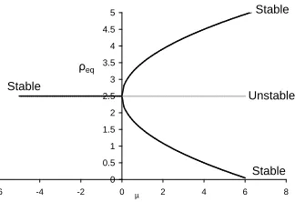
Depending upon the sign ofµ, the steering potential can have two distinct forms. Figure 1 shows the shape of the potential and the corresponding velocity field
whenµ <0 andµ >0. Figure 2 shows the bifurcation diagram for the steering potential indicating a bifurcation from a single local minimum into two local
0 5 10 15 20 0
500 1000 1500 2000 2500 3000
ρ
U
0 5 10 15 20
−500 0 500 1000 1500 2000
ρ
U
(i) (ii)
0 5 10 15 20 0
5 10 15 20
x
y
0 5 10 15 20 0
5 10 15 20
x
y
[image:10.612.141.463.92.396.2](iii) (iv)
Figure 1: Potential and velocity fields (i) potentialµ < 0 (ii) potentialµ > 0 (iii) velocity fieldµ <0 (iv) velocity fieldµ >0
0 0.5 1 1.5 2 2.5 3 3.5 4 4.5 5
-6 -4 -2 0 2 4 6 8
ρeq
µ
Stable
Unstable Stable
Stable
[image:10.612.226.388.478.589.2]The equilibrium states of the potential occur whenever∂U/∂ρi= 0 and∂U/∂zi= 0 . Therefore;
∂U ∂ρi
=−µ(ρi−r) + (ρi−r)3 (18)
∂U ∂zi
=αzi (19)
If µ ≤ 0 equilibrium occurs when ρi = r. If µ > 0 equilibrium occurs when
ρi =r,r±√µ. Therefore, a single ring will bifurcate to a double ring usingµ as a control parameter.
For a function consisting of two variables the stability of the system is
deter-mined from the sign of the determinant of the Hessian matrix [?], D, given in Eq. 20;
D=∂ 2U
∂ρ2 i
∂2U
∂z2 i
−
∂2U
∂ρi∂zi
2
(20)
The conditions for stability are as follows;
(i)D >0,∂2U/∂ρ2
i >0 =⇒equilibrium point is a stable minimum. (ii)D >0,∂2U/∂ρ2
i <0 =⇒equilibrium point is a unstable maximum. (iii)D <0 =⇒equilibrium point is a saddle.
The second derivative of the potential is shown in Eq. 21, 22 and 23;
∂2U
∂ρ2 i
=−µ+ 3(ρi−r)2 (21)
∂2U
∂z2 i
=α (22)
∂2U ∂ρi∂zi
From Eq. 22 asα is positive, ∂2U/∂z2
i >0. From Eq. 21 it can be seen that
∂2U/∂ρ2
[image:12.612.165.445.159.283.2]i ≷ 0 depending on the values of µ. Therefore, the properties of the equilibrium stateρeq are shown in Table 1;
Table 1: Stability of equilibrium states
Bifurcation Equilibrium ∂2U/∂ρ2
i Stability parameter,µ position,ρeq
<0 r >0 stable minimum
>0 r <0 unstable maximum
r+õ >0 stable minimum
r−√µ >0 stable minimum
2.3.1 Linear stability: 1-parameter static bifurcation
In order to determine the linear stability of a system of UAVs subject to such a
1-parameter static bifurcation steering potential we perform an eigenvalue analysis
on the linearized equations of motion assuming that at large separation distances
the repulsive potential can be neglected through scale separation as explained
inSection 2.2. The linear stability analysis will be used to determine the local
behaviour of the system by calculating its eigenvalue spectrum. Therefore, the
equations of motion for the model are re-cast as;
˙
ρi ˙
zi
=
−∂dU S
∂ρi −∂dU S
∂zi
=
f(ρi, zi)
g(ρi, zi)
(24)
f(ρo, zo) = 0 (25)
g(ρo, zo) = 0 (26)
Thus,∇US = 0 at equilibrium. This occurs whenρ
o=rifµ <0,ρo=r, r±√µ ifµ >0 andzo= 0. Defining δρi=ρi−ρo andδzi=zi−zo and Taylor Series expanding about the fixed points to linear order the eigenvalues of system can
be found using;
δρ˙i
δz˙i
=J
δρi δzi (27) where, J= ∂
∂ρi(f(ρi, zi))
∂
∂zi(f(ρi, zi))
∂
∂ρi(g(ρi, zi))
∂
∂zi(g(ρi, zi))
ρo,zo
(28)
The Jacobian,J, is then a 2x2 matrix given by;
J=
−∂2U
∂ρ2
i 0
0 −∂2U
∂z2 i
ρo,zo
(29)
Substituting a trial exponential solution into Eq. 27 we find that;
δρ˙i
δz˙i
= δρo δzo e λt (30)
Therefore, the eigenvalues,λ, of the system are found fromdet(J−λI) = 0.
As shown previously, ifµ <0 equilibrium of the system occurs whenxo= (r,0). Evaluating the Jacobian matrix given in Eq. 29 we find that;
J=
µ 0 0 −α
The corresponding eigenvalue spectrum is therefore;
λ1,2= −α, µ (32)
Asα >0 andµ <0 the eigenvalues are always negative real and the equilibrium position can therefore be considered as linearly stable.
Ifµ >0 equilibrium of the system occurs whenxo1= (r,0), xo2= (r+√µ,0) and xo3 = (r−√µ,0). The Jacobian matrix evaluated at the three different equilibrium positions is given by Eq. 33, 34 and 35 respectively as;
J1=
µ 0 0 −α
(33)
J2=
−2µ 0 0 −α
(34)
J3=
−2µ 0 0 −α
(35)
The eigenvalues forJ1 are;
λ1,2= −α, µ (36)
Considering the pair of eigenvalues in Eq. 36, asα >0 andµ >0 we have one positive eigenvalue so that the equilibrium position is therefore always linearly
unstable.
The eigenvalues forJ2 andJ3 are;
stable.
Figure 3 confirms the linearised stability results showing the phase plane plot
forµ <0 andµ >0.
0 2 4 6 8 10
−10 −5 0 5 10
ρi
zi
0 2 4 6 8 10
−10 −5 0 5 10
ρi
zi
[image:15.612.145.461.181.326.2](i) (ii)
Figure 3: Phase diagram (i)µ <0,r= 5 (ii)µ >0,r= 5
From Fig. 3(i) it can be seen that whenµ <0 we have one stable equilibrium position when xo = (r,0) as indicated by the eigenvalues given in Eq. 31. If the system then bifurcates so that µ > 0, the stable position atxo1 = (r,0) becomes unstable and positions xo2 = (r+√µ,0) and xo3 = (r−√µ,0) are stable agreeing well with eigenvalues given forJ2 andJ3.
2.3.2 Non-linear stability: 1-parameter static bifurcation
To determine the non-linear stability of the dynamical system we consider the
use of Lyapunov methods [24]. We can use this theorem to guarantee the global
stability of the system with convergence to the desired final state. The aim of
thesteering potential is to drive each UAV to the desired equilibrium position
that corresponds to the minimum potential. Therefore, if Lyapunov’s method
mini-mum energy state.
The Lyapunov function,L, for the system is defined in Eq. 38, where US(xi) is given in Eq. 17;
L(xi) =
X
i
US(xi) (38)
In order to ensure the global stability of the system the potential is defined such
[image:16.612.248.359.264.328.2]that the conditions given in Table 2 hold true.
Table 2: Lyapunov’s Second Theorem stability conditions
xi6=xo xi=xo
L(xi)>0 L(xo) = 0 ˙
L(xi)<0 L˙(xo) = 0
The rate of change of the Lyapunov function can be expressed as;
dL dt =
X
i
∂L ∂xi
˙ xi
(39)
Then, substituting Eq. 24 into Eq. 52 it can be seen that;
dL dt =−
X
i
∇Us(xi)2≤0 (40) From Table 2 ifLis a positive definite function and ˙Lis a negative definite the system will be uniformly stable. A problem arises in the use of superimposed
artificial potential functions as ˙L ≤ 0. This implies that ˙L could vanish in a position other than the goal minimum suggesting that the system may become
trapped in a local minimum. In order to ensure that our system is
asymptot-ically stable at the desired goal state the LaSalle principle [25] can be used.
{xi|L˙ = 0}only occurs whenxi=xo, then the goal state is asymptotically sta-ble. Therefore, for the quadratic potential considered in this paper the LaSalle
principle is valid. As we have a smooth well defined symmetric potential field,
equilibrium only occurs at the goal states so the local minima problem can be
avoided and the system will relax into the desired goal position.
2.4
Hopf bifurcation - 1 parameter dynamic bifurcation
In certain engineering applications, a formation of UAVs may be desired to form
a circling surveillance pattern [2]. Frew et al. have shown how this could be
achieved through the use of a Lyapunov guidance vector field approach that
produces a stable convergence to a circling limit cycle behaviour for a system of
UAVs [3] [26]. In bifurcation theory the Hopf bifurcation is a local bifurcation
about a fixed point of a dynamical system that generates a limit cycle as the
bifurcation parameterµchanges sign.
An example of such a Hopf bifurcation is given in Eq. 41 and 42 with Fig. 4
showing an example of the velocity field created whenµ >0. When the bifur-cation parameterµ >0 a pair of complex eigenvalues cross the imaginary axis and the limit cycle behaviour is induced. Asµincreases the size of limit cycle also increases so that we can have a varying size of limit cycle and therefore
surveillance region.
We define the Hopf bifurcation as;
˙
xi=µxi+yi−xi(x2i +yi2) (41) ˙
yi=−xi+µyi−yi(x2i +yi2) (42) The first order control model is shown in Eq. 43 with the repulsive potential
−3 −2 −1 0 1 2 3 −3 −2 −1 0 1 2 3 x y
Figure 4: Hopf Bifurcation: µ >0
˙ xi ˙ yi ˙ zi =
µxi+yi−xi(x2i +y2i)−
∂UR
∂xi −xi+µyi−yi(x2i +y2i)−
∂UR
∂yi −αzi−
∂UR ∂zi (43)
2.4.1 Linear stability: 1-parameter dynamic bifurcation
Similar to the analysis performed insection2.3.1 the velocity field described by
Eq. 43 is recast to determine the linear stability of the system assuming at large
separation distances the repulsive potential function can be ignored. Therefore,
˙ xi ˙ yi ˙ zi =
µxi+yi−xi(x2i +yi2) −xi+µyi−yi(x2i +y2i)
−αzi
=
m(xi)
n(xi)
p(xi)
(44)
Similarly, lettingxo denote fixed points with ˙xi= ˙yi= ˙zi= 0 so that;
n(xo, yo, zo) = 0 (46)
p(xo, yo, zo) = 0 (47) The Jacobian,J, is then a 3x3 matrix given by;
J= ∂
∂xi(m(xi))
∂
∂yi(m(xi))
∂
∂zi(m(xi))
∂
∂xi(n(xi))
∂
∂yi(n(xi))
∂
∂zi(n(xi))
∂
∂xi(p(xi))
∂
∂yi(p(xi))
∂
∂zi(p(xi))
xo,yo,zo
(48)
Thus, it can be shown that;
J=
µ 1 0 −1 µ 0 0 0 −α
(49)
The corresponding eigenvalue spectrum is therefore;
λ1,2,3= −α, µ±i (50) From the eigenvalue spectrum given in Eq. 50 it can be seen that sinceµ < 0 andα > 0 the equilibrium position is linearly stable indicating a stable spiral to that position. Alternatively, if we bifurcate the system and makeµ >0, the eigenvalues are now either positive real or positive real with complex conjugate.
Therefore, as the complex eigenvalues cross the imaginary axis atµ= 0 we have a bifurcation of the system from a stable spiral into the oscillatory limit cycle
motion.
2.4.2 Non-linear stability: 1-parameter dynamic bifurcation
We can again use Lyapunov’s Second Theorem to determine the non-linear
L= 1 2
X
i
x2i (51)
Therefore,
dL dt =
X
i
∂L ∂xi ˙
xi+ ∂L
∂yi ˙
yi+∂L
∂zi ˙
zi
(52)
dL dt =
X
i
ρ2
i(µ−ρ2i)−αz2i
(53)
For µ < 0 and α > 0, ˙L ≤ 0 so that ρi is always decreasing until L = 0 so each UAV would be attracted to the equilibrium position located at the origin
(xi= 0, yi = 0, zi= 0). Alternatively, if µ >0 andα >0, ˙L >0 if ρ2i < µand ˙
L <0 if ρ2
i > µso the system is attracted to a limit cycle of radius,ρi=µ, in thex−y plane withzi= 0.
3
NUMERICAL RESULTS
3.1
Static Bifurcation Formation Patterns
Before considering the UAV application in detail it is useful to demonstrate
numerically the reconfigurable patterns and advantages of the control model
developed by considering a system ofagents. Depending upon the choice of the
free parameters in Eq. 17 (µ, r, α, Cr and Lr) we can achieve three different formations; cluster, ring and double ring. Figure 5 shows the results for a swarm
of 30 agents given random initial conditions with free parameters summarised
−2 −1 0 1 2 −2
−1 0 1 2
x
y
(i)
−5 −3 −1 1 3 5
−5 −3 −1 1 3 5
x
y
−5 −3 −1 1 3 5
−5 −3 −1 1 3 5
y
x
[image:21.612.144.463.171.475.2](ii) (iii)
Figure 5: Formation patterns: (i) cluster formation (ii) ring formation (iii)
Table 3: 1 parameter static bifurcation free parameters
Free Parameter Cluster Ring Double Ring
µ -4 -4 1.5
r 0 3 3
α 50 50 50
zgoal 0 0 0
Cr 1 1 1
Lr 0.5 0.2 0.5
From the results it can be seen that the first formation corresponds to the case
whenµ <0 andr= 0. Theagents in the system are driven towards the origin with the repulsive potential ultimately causing a uniform cluster to form. The
second formation consists of a ring with radius equal to the magnitude that
the pitchfork bifurcation equation is moved on the along the axis (r = 3). In the final formationµ > 0 and the stable equilibrium in the second formation becomes unstable and the system bifurcates into the double rig formation.
3.2
Static Bifurcation Results
-4 -2 0 2 4 -5
0 5 0 50 100 150
x y
ti
m
e
Two Rings: µ = 2, r = 2
[image:23.612.221.391.72.247.2]Ring: µ = -2, r = 2 Cluster: µ = -2, r = 0 Ring: µ = -2, r = 2
Figure 6: Transition between different formations
As it can be seen, the system bifurcates from a ring to two rings to a cluster
then back to a ring. This is achieved through a simple parameter change and is
one of the advantages of using the pitchfork bifurcation equation as a basis for
the artificial potential function. Rather than controlling each UAV individually
the global pattern of the formation can be manipulated viaµ.
3.3
Hopf Bifurcation Results
Figure 7 shows the results for a system of 15 agents interacting through the
hopf bifurcation field as discussed insection 2.3. Theagents in the system are
given random initial conditions and required to fall onto a limit cycle behaviour
−10 0
10
−10 0 100
5 10 15
x y
time (s)
−6 −4 −2 0 2 4 6 −6
−4 −2 0 2 4 6
x
y
[image:24.612.137.465.96.272.2](i) (ii)
Figure 7: Hopf bifurcation results (Cr = 1, Lr = 2, α = 10, zgoal = 0 and
µ= 25) (i) time evolution (ii) final formation
As can be seen from Fig. 7 the 15agentsfall onto the desired limit cycle rotation
and relaxes into constant separation formation.
3.4
Robustness of the Model
As one of the desirable characteristics of the model developed is that the system
−20 −10 0 10 20 −20
−10 0 10 20
x
y
−20 −10 0 10 20
−20 −10 0 10 20
x
y
(i) (ii)
−20 −10 0 10 20
−20 −10 0 10 20
x
y
−20 −10 0 10 20
−20 −10 0 10 20
x
y
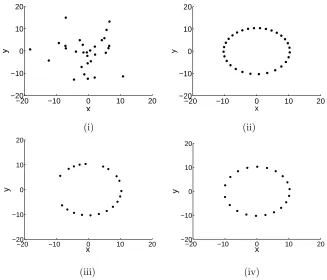
[image:25.612.136.463.73.353.2](iii) (iv)
Figure 8: Robustness of the Model (i) random initial conditions for 30agents
(ii) ring formation (µ=−2,r= 10,Cr= 3 andLr= 5 (iii) failure of 10agents (iv) autonomous reconfiguration of the formation
As can be seen from the results a system of 30agents fall into a ring formation
with radius 10. Figure 8 (iii) shows the random failure of 10 agents with the
assumption that once they fail they are completely removed from the system.
The system will then autonomously reconfigure to a new ring configuration as
shown in Fig. 8(iv).
3.5
Scalable Formation
Another advantage of the model developed is that the systems scales very well
−2 −1 0 1 2 −2
−1 0 1 2
x
y
−2 −1 0 1 2
−2 −1 0 1 2
x
y
(i) (ii)
−2 −1 0 1 2
−2 −1 0 1 2
x
y
−2 −1 0 1 2
−2 −1 0 1 2
x
y
[image:26.612.138.456.76.350.2](iii) (iv)
Figure 9: Scalable formation (i) random initial conditions for 30 agents (ii)
cluster formation (µ = −2, r = 0, Cr = 1 and Lr = 0.5 (iii) addition of 20
agents (iv) autonomous reconfiguration of the cluster formation
Therefore, as shown in the results the system can autonomously reconfigure
3.6
Flexible Formations
The final advantage of the model is that system is flexible to obstacles and can
also alter its pattern through a simple parameter change. By adding in several
circular obstacles it can be shown that we can have a system of 30agents that
will create a cluster formation, autonomously manoeuver to avoid the obstacles,
reconfigure into the cluster pattern and then finally bifurcate into a ring
forma-tion.
A problem with the superimposed artificial potential field method is that the
system may get trapped in a local minimum as noted in section 2.3.2. To
overcome this problem we consider the use of a Gaussian potential function
that creates a spherical potential obstacle with no local minima as defined in
Eq. 54 [27];
Uobs=Coexp−|xi−xobs|/Lo (54) where,xobsrepresents the obstacle position vector andCo,Loare the amplitude and length scale of the obstacle potential respectively.
The coordinate system is altered so that it is translating at constant speed and
from the results shown in Fig. 10 it can be seen that formation ofagents
success-fully falls into the cluster formation, manoeuvres around the obstacles reforming
the cluster formation and then bifurcates into the desired ring formation. The
model can therefore be considered as flexible as the formations have the ability
0
2
4
6
8
10
12
14
16
−2
0
2
x
y
(i)
0
2
4
6
8
10
12
14
16
−2
0
2
x
y
(ii)
0
2
4
6
8
10
12
14
16
−2
0
2
x
y
(iii)
0
2
4
6
8
10
12
14
16
−2
0
2
x
y
(iv)
0
2
4
6
8
10
12
14
16
−2
0
2
x
y
[image:28.612.139.453.73.603.2](v)
Figure 10: Flexible formation (i) random initial conditions (ii) cluster (8s) (iii)
4
UAV APPLICATION
In order to test the model developed we consider a swarm of 10 commercially
available Dragonfly UAV helicopters [28] that are required to fall onto a double
ring formation and then bifurcate into two different ring formations in thex−y
plane, traveling at a final constant speed of 2.7ms−1 whilst ensuring collision avoidance and an equally spaced final formation.
The Dragonfly X6 UAV helicopters have a cruise speed of 2.7ms−1 and maxi-mum turning rate defined as ˙ψmax= 90os−1. It is assumed that the maximum speed and acceleration areVmax = 3ms−1 and ˙vmax = 0.1g respectively. It is also assumed that the position of the UAVs can be determined precisely and
the dynamic control laws developed can accurately control the UAV state.
Although the artificial potential function method is theoretically elegant, Sigurd
[29] points out that the assumption that all UAVs have information on the
position of all other UAVs in the system is unrealistic as the number of UAVs
increase. Each UAV will now have a sensing region that will ensure collision
avoidance and an equally spaced final formation as shown in Eq. 55 and Fig.
11, whereZr is the radius of repulsive zone of influence;
UijR =
X
j,j6=i
Crexp−|xij|/Lr if |xij| ≤Zr 0 if |xij|> Zr
(55)
The control model used is based on a simple first order velocity field tracking
approach that has been used by several authors as a basic way of
transform-ing a desired velocity field into a set of commands that control the speed and
turn rate of each UAV [1, 26, 30]. The desired velocity field explained in
Zr
UAV
[image:30.612.221.390.77.199.2]sensing region
Figure 11: UAV repulsive potential sensing region
(ψi) and speed (Vi) command, assuming the formation is flying at fixed altitude.
Therefore, considering the pitchfork bifurcation described by Eq. 16 the desired
velocity vectors are described by Eq. 56 and 57;
˙
xdesired=µ
xn
ρn
(ρn−r)−
xn
ρn
(ρn−r)3+
X
j,j6=i
Cr
Lr
xij |xij|
exp−|xij|/Lr+u
c (56)
˙
ydesired =µyi
ρn
(ρn−r)− yi
ρn
(ρn−r)3+
X
j,j6=i
Cr
Lr
yij |xij|
exp−|xij|/Lr (57)
where, as the UAVs are desired to move at a constant forward speed equal touc we replacexi with xn =xi−uctand ρi with ρn = (x2n+y2i)0.5 in the steering potential terms.
The desired command speed (Vdesired) and heading angle (ψdesired) are there-fore;
Vdesired = ( ˙x2desired+ ˙y2desired)0.5 (58)
ψdesired= arctan
y˙
desired ˙
xdesired
(59)
x1 x2 x3 x4 = Vi ψi xi yi (60)
A system of first order equations of motion are then solved resulting in a
com-manded speed and heading angle that can be used to control the UAV as shown
in Eq. 61, where the constantsλvandλψare inverse time constants determining the response of each UAV;
˙ x1 ˙ x2 ˙ x3 ˙ x4 =
−λv(Vi−Vdesired) if |v˙i| ≤v˙max −λψ(ψi−ψdesired) if |ψ˙i| ≤ψ˙max
Vicos(ψi)
Visin(ψi)
(61)
In addition as there is a bound on the maximum turning rate and speed there
is turning circle associated with each UAV. The radius of the turning circle is
defined in Eq. 62 so that if the maximum speed and turning rate are 3ms−1 and 90os−1respectively, then the maximum turning radius,R
turning, is
approx-imately 1.9m.
Rturning =
Vmax ˙
ψmax
(62)
In order to estimate that size of the repulsive free parameters,Cr andLr, we can consider the case of 2 UAVs interacting through the repulsive potential
only. Considering a simple 1-dimensional system with position coordinate, X, we know that for X >> 0, dX
dt ≈ Vmax. Therefore, assuming that at close
separation distances the repulsive potential only acts on the UAVs we have;
dX
dt =Vmax− Cr
Lr exp
−X
The minimum separation distance,Xmin, will therefore be estimated by setting
dX
dt = 0 so that,
Xmin=Lrln
Cr
VmaxLr
(64)
In order to ensure collision avoidance, the minimum separation distance between
[image:32.612.167.441.301.383.2]the UAVs in the formation must be 2×Rturning = 3.8m. The repulsive po-tential constants,Crand Lr, are therefore chosen to ensure that the minimum separation,Xmin, is greater than this value. Each UAV is given random initial conditions in thex−y plane with initial speed of 2.7ms−1 and random initial heading angles. The free parameter values are summarised in Table 4.
Table 4: 1 parameter static bifurcation free parameters
f ormation time (s) µ r Cr Lr λv λψ ZR double ring 0-200 100 30 73 20 1 1 45
ring 200-400 -1 40 73 10 1 1 45
ring 400-600 -1 50 73 10 1 1 45
From the results shown in Fig. 12, 13 and 14 it can be seen that the formation
successfully creates the desired equally spaced double ring formation and
bifur-cates into the two ring formations. Figure 12 shows the final formation, whereas
Fig. 13 shows the time evolution for each formation. It can also be seen from
Fig. 14 that the formation relaxes into a constant separation distance for each
460 480 500 520 540 560 580 600 620 −80 −60 −40 −20 0 20 40 60 80 x (m) y (m)
100010201040106010801100112011401160 −80 −60 −40 −20 0 20 40 60 80 x (m) y (m)
[image:33.612.144.471.76.161.2]154015601580160016201640166016801700 −80 −60 −40 −20 0 20 40 60 80 x (m) y (m)
Figure 12: UAV formations in final state (i) double ring (ii) ring (radius = 40m
(iii) ring (radius = 50m)
0 200 400 600 800 1000 1200 1400 1600 1800
−100 0 100 x (m) y (m) (i)
0 200 400 600 800 1000 1200 1400 1600 1800
−100 0 100 x (m) y (m) (ii)
0 200 400 600 800 1000 1200 1400 1600 1800
−100 0 100 x (m) y (m) (iii)
0 200 400 600 800 1000 1200 1400 1600 1800 −100 0 100 x (m) y(m) (iv)
Figure 13: UAV results (i) random initial conditions (ii) formation after 200s
[image:33.612.141.472.204.559.2]0 100 200 300 400 500 600 700 800 0
50 100 150
time (s)
|X
ij
|
[image:34.612.206.401.78.215.2]|X min|
Figure 14: UAV separation: indicating an equally spaced final formation with
collision avoidance
Therefore, through the use of a velocity field tracking approach we are able to
generate a real set of commands that can control a swarm of UAVs, allowing a
reconfigurable equally spaced formation with collision avoidance assured.
5
CONCLUSION
It has been shown how a behavioural based control method can be used to
create various patterns for a formation of UAVs and has the advantages of being
robust, scalable and flexible. Dynamical systems theory is used as the basis of
the control method with the new approach of bifurcating potential fields used
for pattern formation and reconfigurability. A first order velocity field is used to
command each UAV based on a steering and repulsive potential field. It is shown
that there exists a scale separation between the steering and repulsive potential
so that each UAV moves under the influence of a long range steering potential
but with short range collision avoidance. Using this the stability of the system
was demonstrated analytically to ensure that desired behaviours always occur.
To demonstrate the algorithm developed we consider the control of 10 UAVs
bifurcate into two different ring formations traveling at constant speed whilst
also ensuring collision avoidance. A simple 1st order velocity field tracking
approach is used to track the desired velocity field and generate a set a real
commands that control the aerodynamic surfaces of the UAV. We consider the
use of 10 commercially available UAV helicopters that have maximum turning
rate of 90os−1. The numerical results successfully show the formation of an equally spaced double ring of UAVs that then bifurcates into two different ring
formations, traveling at constant speed with collision avoidance ensured.
References
[1] C. R. McInnes. Velocity field path-planning for single and multiple
un-manned aerial vehicles. The Aeronautical Journal, 107(1073):419–426,
2003.
[2] R. Beard, D. Kingston, M. Quigley, D. Snyder, R. Christiansen, W.
John-son, T. McLain, and M. Goodrich. Autonomous vehicle technologies for
small fixed wing UAVs. In2nd AIAA Unmanned Unlimited Systems,
Tech-nologies, and Operations, San Diego, California, 15 - 18 September 2003.
[3] E. Frew, D.A. Lawrence, and S. Morris. Coordinated standoff tracking of
moving targets using lyapunov guidance vector fields.Journal of Guidance,
Control and Dynamics, 31(2):290–306, March-April 2008.
[4] R. Teo, J.S Jang, and C.J. Tomlin. Automated multiple UAV flight - the
stanford dragonfly UAV program. In 43rd IEEE Conference on Decision
and Control, Atlantis, Paradise Island, Bahamas, 14 - 17 December 2004.
[5] M. Quigley, M.A. Goodrich, S. Griffiths, A. Eldredge, and R.W. Beard.
Target acquisition, localization, and surveillance using a fixed-wing
mini-UAV and gimbaled camera. InIEEE International Conference on Robotics
[6] A. Ollero and L. Merino. Control and perception techniques for aerial
robotics. Annual Reviews in Control, 28(2):167–178, October 2004.
[7] O. Ilaya, C. Bil, and M. Evans. Control design for unmanned aerial
ve-hicle swarming. Proc. of the Institution of Mechanical Engineers, Part G:
Journal Aerospace Engineering, 222(4):549–567, 2008.
[8] R. A. Brooks. A robust layered control system for a mobile robot. IEEE
Journal Of Robotics And Automation, 2(1):14–23, 1986.
[9] T. Balch and R.C. Arkin. Behavior-based formation control for multi-robot
teams. IEEE Transaction on Robotics and Automation, 14(6):926–939,
December 1998.
[10] J.H. Reif and H. Wang. Social potential fields: A distributed
behav-ioral control for autonomous robots. Robots and Autonomous Systems,
27(3):171–194, 1999.
[11] K. Han, J. Lee, and Y. Kim. Unmanned aerial vehicle swarming control
using potential functions and sliding mode control. Proc. of the
Insti-tution of Mechanical Engineers, Part G: Journal Aerospace Engineering,
222(6):721–730, 2008.
[12] O. Khatib. Real-time obstacle avoidance for manipulators and mobile
robots. The International Journal of Robotics Research, 5(1):90–98, 1986.
[13] A Badawy and C.R. McInnes. Robot motion planning using hyperboloid
potential functions. InWorld Congress on Engineering, London, UK, July
2-4 2007.
[14] S.S. Ge and Y.J Cui. Dynamic motion planning for mobile robots using
po-tential field method. Autonomous Robots, 13(3):207–222, November 2002.
[15] D.J. Bennet and C.R. McInnes. Pattern transition in spacecraft formation
International Symposium on Formation Flying, Missions and Technologies,
Noordwijk, The Netherlands, April 23-25, 2008.
[16] A. Badawy and C.R. McInnes. On-orbit assembly using superquadric
po-tential fields. Journal of Guidance, Control, and Dynamics, 31(1):30–43,
2008.
[17] D. Izzo and L. Pettazi. Autonomous and distributed motion planning for
satellite swarm. Journal of Guidance, Control, and Dynamics, 30(2):449–
459, 2007.
[18] W.J. Crowther. Rule-based guidance for flight vehicle flocking. Proc. of
the Institution of Mechanical Engineers, Part G: Journal Aerospace
Engi-neering, 218(2):111–124, April 2004.
[19] P. Basu, J. Redi, and V. Shurbanov. Coordinated flocking of UAVs for
improved connectivity of mobile ground nodes. InIEEE Military
Commu-nications Conference, volume 3, 31 Oct - 3rd Nov 2004.
[20] R. Olfati-Saber. Flocking of multi-agent dynamic systems: Algorithms and
theory. IEEE Transactions of Automation Control, 51(3):401–420, March
2006.
[21] K.H. Tan and M.A. Lewis. Virtual structures for high precision cooperative
mobile robotic control. In IEEE/RSJ International Conference Intelligent
Robots and Systems, volume 1, pages 132–139, Osaka, Japan, 4-8 November
1996.
[22] M. R D’Orsogna, Y. L Chuang, A. L Bertozzi, and S. Chayes. Self-propelled
particles with soft-core interactions: patterns, stability and collapse.
Phys-ical Review Letters, 96(10):14302–1 – 14302–4, March 2006.
[23] D.W. Jordon and P. Smith.Nonlinear Ordinary Differential Equations: An
[24] R. E. Kalman and R. E. Bertram. Control system analysis and design via
the second method of lyapunov: (i) continuous-time systems (ii) discrete
time systems. Transactions ASME Journal Basic Engineering, 82:371–393,
June 1960.
[25] J.P. LaSalle. An invariance principle in the theory of stability.International
Symposium on Differential Equations and Dynamical Systems, pages 277–
286, 1967. Ed. New York: Academic Press.
[26] D.A. Lawrence, E. Frew, and J. Pisano. Lyapunov vector fields for
au-tonomous unmanned aircraft flight control. Journal of Guidance, Control
and Dynamics, 31(5):1220–1229, September-October 2008.
[27] F. McQuade. Autonomous control for on-orbit assembly using artificial
potential functions. PhD thesis, University of Glasgow, 1997.
[28] Dragonfly X6 UAV RC Helicopter.
http://www.draganfly.com/uav-helicopter/draganflyer-x6/, 18th December 2008.
[29] K. Sigurd and How. J. UAV trajectory design using total field collision
avoidance. InAIAA Guidance, Navigation and Control Conference, August
2003.
[30] G. Gowtham and K. S. Kumar. Simulation of multi UAV flight formation.
In24th Digital Avionics Systems Conference, volume 2, 30th October - 3rd