Forward looking versus myopic regional computable general equilibrium models : how significant is the distinction?

S

TRATHCLYDE

D

P

E

D

E

U

S

G

FORWARD LOOKING AND MYOPIC REGIONAL

COMPUTABLE GENERAL EQUILIBRIUM MODELS. HOW

SIGNIFICANT IS THE DISTINCTION?

B

PATRIZIO LECCA, PETER McGREGOR AND

KIM SWALES

1

Forward Looking and Myopic Regional Computable General

Equilibrium Models. How Significant is the Distinction?

Patrizio Leccaa,*

Peter G. McGregora,b

and

J. Kim Swalesa

a _{Department of Economics, University of Strathclyde, United Kingdom.} b

Fraser of Allander Institute and Department of Economics, University of Strathclyde, United Kingdom.

*_{Corresponding author: Department of Economics, University of Strathclyde, Rm. 4.27, Sir William Duncan}

Building 130 Rottenrow, Glasgow G4 0GE. Tel: 44(0)1415483962 E-mail:[email protected].

2

Abstract

We present a stylized intertemporal forward-looking model able that accommodates key regional economic features, an area where the literature is not well developed. The main difference, from the standard applications, is the role of saving and its implication for the balance of payments. Though maintaining dynamic forward-looking behaviour for agents, the rate of private saving is exogenously determined and so no neoclassical financial adjustment is needed. Also, we focus on the similarities and the differences between myopic and forward-looking models, highlighting the divergences among the main adjustment equations and the resulting simulation outcomes.

JEL classification: C68; D58; D91; R10

3

1. Introduction

Regional Computable General Equilibrium (CGE) models solve complex optimization

problems within individual time periods in order to determine a complete allocation of a

region’s resources between alternative uses. However, such models often lack

forward-looking expectations and this has been presented as a weakness (Partridge and Rickman,

1998; 2010). In this paper we attempt to identify how significant the lack of forward looking

expectations is in this setting. In particular, we build a stylized forward-looking CGE model

applicable in a regional context. Results from simulations using this model are then compared

to those from a similar model where the adjustment processes between periods have a myopic,

backward-looking, recursive-dynamic structure.

In this comparison of results we find the simulation differences are small. The long-run

equilibria are identical. Furthermore, the adjustment paths generated by the two models are

not radically different. We suggest two possible reasons why the importance of incorporating

forward-looking expectations into regional CGE models might have been overstated. First, in

previous comparisons using national models, the fully dynamic forward-looking model has

often been compared to either a static model or one with passive investment. Second, the

usual mechanism and closures that are applied in national inter-temporal CGE models

misrepresent the adjustment mechanisms that typically occur within an individual region.

The structure of the remainder of the paper is as follows. In Section 2 we provide a

background discussion of the theoretical issues. In Section 3 we outline the model structure.

In Section 4 we deal with the calibration method. In Section 5 we present the simulation

4

2. Background

The theoretical structure of many intertemporal forward-looking CGE models is that

described in Abel and Blanchard (1983). Such a model can be solved as a decentralized

economy where consumption decisions are made by intertemporal optimizing households,

with savings and investment decisions separated. Financial balance equilibrium is maintained

through adjustment of either foreign borrowing, the interest rate, or by means of fiscal policy

that, in turn, affects the financial wealth of households. Firms’ forward-looking behaviour

influences their investment decisions which depend on the tax-adjusted Tobin’s q.

Furthermore, in their stylized form, such models usually make households fully liable for the

financial needs of the system. Hence, household savings would cover not only the needs of

domestic investment, but also, ultimately, trade and Government deficits. Accordingly,

households have to save as much as is required to clear the financial sector which, in turn,

implies the imposition of a balance of payments constraint.

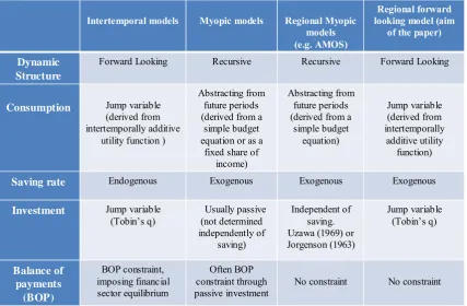
In fact, forward-looking models are frequently calibrated on national data and their

specification is nowadays becoming standardized. Their key characteristics are summarized in

the first column of Table 1. However, the application of model specifications that imply a

zero balance of payments and a savings rate obtained endogenously through financial balance

equilibrium, may be inappropriate in a regional context since regions are likely to differ from

the country as a whole in a number of significant respects.

It is widely recognised that regions are more open than nations and that regional economies

typically do not have the full range of macroeconomic policy levers (and many regions have

5

national Government so that policy instruments and some macroeconomic adjustment

mechanisms, whose incorporation is uncontroversial in a national model, cannot routinely be

assumed to apply to the case of a region1. Furthermore, regions, unlike nations, do not face a

binding balance of payments constraint. There are at least two reasons for this. Firstly, the

balance of payments is not required as a policy target since regions usually belong to a

common currency area and to a nationally integrated financial system. As a result, fiscal and

monetary policies cannot be used to produce balance of payments adjustments through control

variables such as exchange rates, reserve assets and interest rates. Secondly, the subvention

that regions receive from higher level authorities, such as centralized Government and the EU,

may cause some distortionary effects so that a rigorous theory of the composition of the

balance of payments is not really a regional issue. As pointed out by McGregor et al (1995),

such subventions are key determinants of the regional trade deficits. As long as national

governments are credibly committed to the maintenance of the monetary union, regions do

not face binding balance of payments constraints. In the UK context, for example, it is

well-known that Northern Ireland has over many years maintained a balance of payments (and

public sector) deficit that would be unsustainable for a national economy. But the UK

government is committed to the union and essentially underwrites this position.2

The point is that forward-looking models impose balance of payments equilibrium in order to

maintain financial sector sustainability, but regions are not obliged to undergo this form of

financial adjustment. For instance, if a region faces an unsustainable position in which a net

foreign debt is accompanied by a persistent trade deficit, it is not required to adopt rigorous

adjustment in order to produce a trade surplus to cover interest payments because there is no

1_{Even though some nations are likely to behave as regions (European countries for example).} 2

6

superior authority to impose it. A superior institution such as central Government, may reduce

the subvention to reduce its level of debt and, in turn, the region’s implicit (unobservable)

debt. However, this is a process that occurs outside the region. It implies that any adjustment

is imposed exogenously, from outside the region; it does not operate as an automatic,

endogenous adjustment mechanism. This also means that the Ricardian implication of the

fiscal deficit which is usually embedded in consumers’ optimal decisions might be unrealistic;

typically a regional (i.e. sub-national) Government which has no significant devolution of tax

or borrowing powers, cannot finance its expenditure by levying taxes or issuing bonds. In this

context regional policy is exogenous to the region, reflecting the subvention received from

outside the region.

Of course, given widespread movement towards greater devolution within the EU, more

regions will be given the responsibility, and be equipped with the corresponding instruments,

to deal with the reduction in subventions, thereby introducing specific sustainable targets that

might bring about a partial endogenous financial adjustment operating within the region.

However, only when regions start to behave like countries belonging to a common currency

area, e.g. the European countries, does the balance of payments begin to be a matter at the

regional level, and any adjustment in internal and foreign assets ceases to be exogenously

determined. However, this does not necessarily imply that the traditional approach to the

balance of payments becomes appropriate. Even in this case, and for such regions, it may be

inappropriate to impose full interregional and international payments constraints.

Our view is that in a regional intertemporal model, the treatment of internal and external debt

should differ from the usual application in a corresponding national model. Thus, in a stylized

7

deficit flows, should not be involved in the process that determines financial adjustment

within the region. This also means that the role of savings should differ from that played in

standard applications. In a region, the household savings decisions are independent of the

regional financial system. In fact, such decisions are more likely to be affected by national

adjustment which is, of course, exogenous in a single small, open regional economy model.

The intertemporal model developed in this paper maintains forward-looking behaviour for

both households and firms, and investment and saving decisions are kept separate. However,

unlike standard applications, in our formulation savings follow the Solow-Swan assumption

so that the rate of savings is exogenous. This does not prevent the absolute level of savings

from varying through time. The key characteristics of this model are summarised in the final

column of Table 1.

We compare simulation results from myopic and forward-looking models. Under particular

circumstances, we find that both models produce the same long-run steady state equilibrium.

This outcome differs from those reported in the existing literature (e.g., Go, 1994; Devarajan

and Go, 1998 ) where the long-run impact differs in both models. Major concern over

incorporating forward-looking expectations has arisen when the policy to be evaluated has

intrinsic long-run effects (as in trade liberalization policy, for example). Go (1994) and

Devarajan and Go (1998) argue that myopic models fail to capture dynamic policy gains and,

consequently, produce both inaccurate and incorrect results. For example, Devarajan and Go

(1998) claim to demonstrate that the welfare gains of eliminating trade tariffs are greater in

forward-looking models than in static models3.

8

However, the underlying reason for these results is related, as we explain later, to the

asymmetric model specifications incorporated in both models. Indeed, it would seem that the

intertemporal forward-looking model has generally been compared to the simple static case

that lacks any optimal capital adjustment rule, so that investment is either crudely assumed

fixed to the base year level or is passive. The characteristics of this model are summarised in

column 2 of Table 1. Consequently, myopic and forward-looking models have produced

results that differ even in the long-run. In our approach we find the same long-run equilibrium

for comparable myopic and the forward-looking models, although the transitional paths differ.

Independently of the dynamic structure, forward-looking and myopic regional models should

incorporate a separate investment function and the investment decision must be determined

independently of the savings decision.

The myopic model used in this example, which follows the usual AMOS closures (McGregor

et al 1995, 1996), allows investment to respond to the current rate of return to capital (column

3 of Table 1). In addition the analysis is enriched by assuming labour supply adjustment

through migration, and by investigating the role of different labour market closures. CGE

models based on myopic expectations have been criticised by the supporters of

forward-looking models because of the intertemporal inconsistency involved in assuming

backward-looking expectations. The models solve complex optimization problems within periods in

order to determine the best allocation of resources. However, between periods they remain

myopic, with consumption, saving and investment decisions abstracting from future periods

(Devarajan and Go, 1998). We argue in this paper that such differences are the result of the

different adjustment mechanisms incorporated into these models and not, in fact, the

9

We proceed by specifying illustrative regional intertemporal (column 4) and myopic (column

3) models, calibrating them to a common database, and subjecting them to an identical

disturbance. This allows us to conduct a systematic comparison of their simulation properties,

and thereby isolate the significance of the distinction between myopic and forward looking

regional models.

Furthermore, in order to clarify the significance of our particular assumptions about the nature

of regional adjustment processes, we also develop both forward looking and myopic regional

models that share key characteristics of the national models identified in Table 1. In

particular, we impose a regional balance of payments constraint and saving behaviour that

makes regional households responsible for financial equilibrium. By calibrating these models

to the same database and subjecting them to the same disturbance as our preferred

specifications for regional models, we can reveal the true source of key model properties. This

allows us to identify the significance of alternative assumptions about macroeconomic

processes, as well as alternative assumptions about expectations formation, for the properties

of models of regional economies.

3. Model Description

A single-region dynamic CGE model is presented in this section. The complete mathematical

representation is provided in Appendix A (A.1 - A.77).

Parameterisation is implemented through the well-known calibration method using a Social

10

prices at which excess demand is zero is the result of an optimization process where market

clearing prices equal marginal costs in each sector.

Three economic activities or sectors are considered: Primary, Manufacturing and Services. No

distinction is made between traded and non-traded sectors. Sardinia is a very small open

economy and almost all sectors compete in interregional and international markets. Even

health care services, traditionally a sheltered sector, are now inter-regionally traded.

Production inputs include primary factors and intermediate purchases. The model includes

three domestic institutional sectors: Firms, Households and Government. External institutions

are split into the Rest of Italy (ROI) and Rest of the World (ROW). We adopt assumptions

typically used for a small open economy. The region is too small to affect prices in

international and interregional markets and, as a consequence, the ROI and ROW prices are

taken to be exogenous. The behaviour of Households and Firms is based on intertemporal

optimization with perfect foresight. Government is a consolidated sector merging central and

local Government levels whose expenditure can be either the result of an optimization

process, where Government is simply treated as a new consumer maximizing utility subject to

the budget constraints, or it is held constant in real terms.

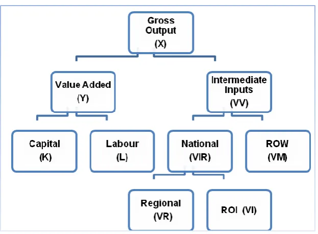
Production. The model’s production structure is illustrated in Figure 1. Intermediate inputs

(VV), labour (L) and capital (K) constitute the production inputs of the model. L and K are

combined in a CES production function in order to produce value added, Y, allowing for

substitution among primary factors of production (A.17). The demand for L and K is obtained

from the first order condition of profit maximization. This implies that the demand for both K

and L is positively related to the volume of value added, Y, and is a decreasing function of

11

(A.14), so the combination of value added and intermediate inputs can be shown with an

L-shaped isoquant. Intermediate goods produced locally or imported are considered as imperfect

substitutes. Basically, we mix regional and imported goods under the so called Armington

assumption through a CES function. The demand function for regionally produced and

imported intermediate inputs (from ROI and ROW) derives from the solution of a cost

minimization problem (A.19-A.22). Regional commodities supply is bought by industries and

by domestic and external institutions (A.24). That is to say, each industry in the region

produces goods and services that can be exported or sold in the regional market. An export

demand function closes the model where the foreign demand for Sardinian goods depends on

the terms of trade effect and on the export price elasticity (A.23).

Investment. Thisfollows Hayashy (1982) with the rate of investment as a function of marginal

q (or average q)4, the ratio of the value of firms (VF) to the replacement cost of capital Pk∙K.

With adjustment costs that are quadratic in investment, the economy does not adjust

instantaneously to the desired level of capital stock. Accordingly, firms respond to the shock

by making continuous small investments over time. The dynamic path of investment is the

result of an intertemporal programme that seeks to maximize VF subject to the capital

accumulation equation, ̇, (A.50). The value of firms, VF, is given by the present value of the

net income or cash flow, CF, that is to say, the capital income less investment expenditure

. The investment expenditure equation (A.45) is defined as a function of the adjustment

cost ( ) (A.48) as in Devarajan and Go (1998), Go (1994) and Hayashi (1982). The

4 _{As we are assuming that the firm is price taker, the marginal q is equal to the average q. For more detail see}

12

solution to this intertemporal problem5 produces the time path of investment (A.46) along

with the law of motion of the costate variable (A.47).

Consumption. Individuals optimise their lifetime utility function of consumption, C (A.26)

subject to a lifetime wealth. Once the optimal path of consumption is obtained from the

solution of the intertemporal problem (A27), aggregate consumption is allocated within each

period and between different groups through a CES function (A.34). Household demand for

regional and imported goods (A.35 and A.36) is the result of the intra-temporal cost

minimization problem. According to the dynamic budget constraint, the discounted present

value of consumption must not exceed total household wealth, W. The model distinguishes

between financial wealth (FW) and non-financial wealth (NFW). So total Wealth, W, is given

by:

(1)

The NFW accumulate as follow:

( ) (2)

5

The optimality conditions (or the canonic system which gives the system of differential equations in the optimal control problem) are given by the first order condition of the Hamiltonian in current value:

A.

( )

B. ̇

̇ ( )

C. (trasversality condition)

13

where is the net labour income plus transfers of income from internal and external

institutions. FW, unlike in the standard applications, is accumulated through saving, S as

follows:

( ) (3)

and

(4)

where is capital income, is total household current income (that is, ) whilst

mps is a parameter calibrated from the SAM. This way of proceeding, although allowing us to

deal with an exogenous rate of household saving, is wholly consistent with forward-looking

consumption behaviour. In fact, consumption still depends on lifetime income. That is to say,

consumers base consumption decisions on expected future income even thought now, saving

is not affected by investment and from the current account situation.

In the traditional approach, financial wealth is obtained by assuming asset equilibrium so that

financial wealth accumulates according to the following:

( ) (∑ ) (5)

where FD is the fiscal deficit and TB is the trade balance. Then ∑ gives us

endogenous saving which replaces equation (2). This means that household financial wealth is

14

∑ ₍₆₎

In others words the wealth derived from asset holdings consists of the value of firms (VF),

public assets (GD) and foreign assets (D). The value of firms represents the wealth generated

from assets that consist of domestic firms’ shares. Foreign assets reflect holdings of foreign

firms’ shares. The value of public assets is derived from Government bonds issued to finance

the fiscal deficit.

In this formulation, as described in equation (3) and (4), the balance of payments still clears

and we do not need to impose any balance of payments adjustment because the total

absorption equation is sufficient to guarantee equilibrium in the payments account since we

are not considering money as a commodity. In contrast, implicit in equation (5) is the

imposition of a balance of payments adjustment because savings are determined

endogenously according to the financial needs of the regional system. This method is

incoherent if a regional context is considered. As we have said in the introduction, it is

plausible that the regional savings rate depends very much on the national economy and,

unlike countries there is no saving-investment association. Furthermore, regions are unlikely

to face a balance of payments problem because the multiregional capital market is highly

integrated and capital moves freely across regions.

In other intertemporal models household savings have also been determined as a fixed share

of income, as for instance in Go, (1994). He exploits Abel’s and Blanchard’s (1983)

equivalence to delete the household budget constraint, solving the model as a centralized

15

endogenous. We can also run the model as a master plan, not considering the motion equation

of the state variable W (see Section 4).

Domestic private Assets. From Hayashi’s (1982) work we know that if the firm is a price

taker, then marginal q is equal to average q. Therefore we can specify the shadow price of

capital as the ratio of the value of the firm VF to its capital stock K (A.59).

Foreign and public assets. The common hypothesis is that both internal and external debt

accumulates over time in accordance with the level of deficit and interest payments.

Moreover, terminal conditions for assets are imposed in order to avoid Ponzi games. As many

CGEs are calibrated on steady state equilibrium, the need to maintain a sustainable position

may generate a dataset that does not reflect the real situation of the region. For instance, the

calibration of the foreign asset/debt is derived by imposing regional sustainability with respect

to foreign creditors or debtors. In doing this, if the regional SAM registers a trade deficit, we

need to impose (and suppose) that, in the past, the region has run in surplus for many years in

order to accumulate assets; the presence of a trade surplus should imply foreign debt. But

several regions are in a permanent Ponzi game condition. If we do not take this situation into

account, the quantitative nature of the results may change. So, if foreign debt accumulates

according to the following: ̇ and the trade balance TB is positive (so a trade

deficit), a sustainable long-run position should require interest-bearing foreign assets held by

the private sector. Alternatively, a negative TB (trade surplus) in the long-run would be able to

cover interest payments on any outstanding foreign debt. In a regional context we may

suppose, instead, those capital inflows necessary to cover the trade deficit are partially

constituted by subvention on which no interest is paid and that, therefore, will not reduce

16

deficits exist on both interregional and international side. Sardinia is a region that receives

extensive capital subvention from the EU and the Italian Government: any payments from the

Social or Structural funds of the EU are matched by the National Government. Such capital

inflows are free of charge and not determined by the desire of an investor to acquire Sardinia

assets. In this case the change in debt that may affect the sector financial balance should be

net of this capital inflow. In modelling this situation we may assume that a proportion of

debt, , is the amount of subvention that the region receives from the National Government or

EU, and not because there is the desire to invest in the region:

̇ ( ) (7)

So the debt accumulates only if ( ) and the net foreign debt is equal to the

gross debt less the accumulated subvention on the assets in the gross debt.

As regards Government debt or assets, because Sardinia has an internal deficit, according to

the usual calibration that imposes sustainability of fiscal deficits, we would need to suppose

the presence of Government assets which reduce the total assets available for private agents.

However for the same reasons, as explained above, we consider an “unsustainable” position

as one in which the debt is going to accumulate net of the resources that the region receives

from outside of the region (A.62).

Labour market regimes and labour supply. The model incorporates three labour market

closures reflecting the form of wage setting: regional wage bargaining (RB), national

bargaining (NB) and fixed real wage, (FRW). The wage-setting functions are defined below,

17

the steady state and u is the regional unemployment rate. is the elasticity of wages related to

the level of unemployment rate and it can also be interpreted as an index of wage flexibility.

{

[ ] ( ) ( )

( ) ( )

(8)

In the regional wage bargaining regime, the labour market is defined by the wage curve

(Blanchflower and Oswald, 1994) according to which wages and unemployment are

negatively related6. Thus regional wages are directly related to workers’ bargaining power and

respond to excess demand for labour. NB is a typical Keynesian closure. It assumes that the

nominal wage is fixed at the base year level. This could be motivated by a system in which

the nominal wage is fixed at the national level by the presence of a nation-wide bargaining

system (Harrigan et al., 1991). FRW is used to obtain an alternative counterfactual analysis,

reflecting a “real-wage-resistance” hypothesis, where bargaining ensures that the purchasing

power of wages remains stable over time.

As regards demographic developments and labour supply, we assume that there is no natural

population change, but the labour force adjusts through a migration model commonly

employed in AMOS (Harrigan et al.1996, McGregor at al. 1996). The migration model

assumes the form specified in Layard et al. (1991) and Treyz et al. (1993) where the net

migration flow is taken to be positively related to the gap between the log of regional and

national ( wN/cpiN ) real wages, and negatively related to the difference between the log of

regional and national, (uN), unemployment rates:

18 [ ( ) ( ̅ )] * (

) ( ̅

̅̅̅̅ )+ ( 9 )

where nim is the rate of net migration and is a parameter calibrated in order to ensure zero

net migration in the base period. and are elasticities that measure the impact of the gap

between the logs of regional and national unemployment and real wage rates.

4. Calibration

The model calibration process assumes the economy to be initially in steady state equilibrium.

The parameters of the models are obtained from the SAM by means of the usual calibration

method. Since, in a deterministic approach, some of the parameters remain unspecified, we

need to find them from outside the model, so the elasticities of substitution and other

behavioural parameters are based on econometric estimation or best guesses. For all sectors,

trade elasticities are set equal to 2 whilst production elasticities are equal to 0.3. The wage

curve elasticity is set to -0.033, following to a recent econometric estimation reported in

Devicienti et al. (2008), whilst in the migration function and are set equal to -0.08 and

0.06, respectively7. These elasticities are commonly used in AMOS and econometrically

estimated by Layard et al. (1991).

7 _{We are using parameters estimated on UK data. However this can be a good approximation for European}

countries. For example, the values of these parameters are almost double for the US economy (see Treyz et al. 1993).

19

The values of adjustment cost parameters8 and in equations (A.46-9) are assigned values

0 and 1.5, respectively. The World interest rate is set to 0.04, the rate of depreciation to 0.07

and the inter-temporal elasticity of substitution is equal to 1.5. Given the value of total

investment, J, as supplied by the System of National Accounts (ISTAT, 2005) through the

capital matrix9, KMi, j, the equality condition with total investment by origin in the SAM holds

true. The price of capital goods, Pk, is set equal to unity since the benchmark prices on the

consumption side are set equal to one. W corresponds to the discounted flow of current

income, NFW to the discounted flow of net labour income, and FW is obtained by

maintaining asset equilibrium. By imposing equality10 between the rate of return to capital rk

and the user cost of capital11, uck, from the constraint equations (A.28), A(.40), (A.45-49),

(A59) and (A.62-67), we obtain consistent values for the variables I, K, , W, NFW and FW.

The model is solved by applying the usual procedure in solving an infinite time horizon

model, by imposing steady state conditions at a specific point in time. In the first periods we

impose factor constraints in order to identify short-run impact; however the transitional

pathway is the result of the discrete time solution of the model12.

8 _{In many applications the parameter is set to zero. The value of is set to 0.9 in Dissou (2002) in a model}

of Senegal and in Go (1994) and Devarajan and Go (1998) in their model of Philippine is set at 2.

9 _{For detail about the construction of the Sardinian capital matrix, see Garau and Lecca (2008).}

10 _{The equality between rk and uck is necessary since we are proposing the same calibration method for the}

myopic and the intertemporal model.

11 _{Given that the interest rate and the depreciation rate are fixed, the user cost of capital depends on the variation}

of the capital good price, Pk.

12

20

The myopic model developed here, and which is compared with the intertemporal model, is

not obtained recursively, rather the equations of the model are solved simultaneously for a

given finite time horizon. Since the myopic model does not incorporate jumping variables the

results correspond, of course, to those of the recursive one. In addition, the model

incorporates an adjustment cost function through which investment is determined

independently of savings. The adjustment rule introduced in the myopic model follows that

employed in AMOS (McGregor et al., 1996) which is consistent with the neoclassical

formulation developed in Jorgenson (1963) and Eisner-Stroz (1963); the optimal path of

investment is derived through the accelerator mechanism :

[ ]

where is the desired level of capital. This is wholly compatible with the Uzawa

formulation of adjustment cost where the investment capital ratio ( ) is determined by the

rate of return to capital (rk) and the user cost of capital (uck), allowing the capital stock to

reach its desire level in a smooth fashion over time:

( )

Although Uzawa’s formulation and Tobin’s q theory are formally different, they are in

essence “equivalent,” as noted in Hayashi13

(1982).

21

The myopic model can also be run for two static conceptual time closures: the Short-Run

(SR) and the Long-Run (LR). In the SR, capital and labour supplies are fixed at their base

year values and the initial distribution across sectors is also maintained; in the LR, factor

constraints are relaxed allowing for complete capital and labour adjustment. Capital stock is at

its optimum level, with rental rates equal to user cost of capital. With regard to labour supply,

the population is fully adjusted so that the system exhibits zero net migration. We also allow

for perfect mobility across sectors. This kind of adjustment is quite similar to those reported

in AMOS, a CGE for Scotland (McGregor et al., 1996).

5. Simulation strategy

We present several simulations in order to compare different forward-looking model

specifications (which are declared by an FL prefix). Comparisons between forward-looking

and myopic models (MYP prefix) are also carried out. In all simulations the disturbance takes

the form of a 10% increase in interregional exports. We prefer a simple demand shock since

this simplifies the analysis (and we do not focus here directly on policy issues), but its aim is

to highlight the main differences that may arise by changing the dynamic structure of the

model and some household closure rules.

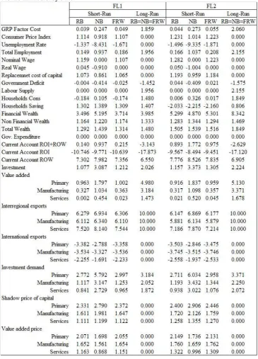
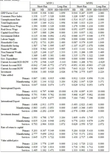
We present the proportionate changes from base year values for a set of key economic

variables in Tables 2 and 3 for the intertemporal and myopic models, respectively. In the

tables, only the short-run and long-run results are reported, along with outcomes related to the

three labour market regimes: Regional Bargaining (RB), National Bargaining (NB) and Fixed

Real Wage (FRW). We distinguish between models with fixed saving rate (FL1 and MYP1)

22

sto the model that closer to a regional economic system, while the second specification should

be instead apply only in the national context. The main difference between the regional

forward looking model (FL1) and its myopic counterpart (MYP1), and the forward looking

(FL2) and myopic (MYP2) models run with national closure is in the financial adjustment

process and its implication for the balance of payments.

In FL1, we try to design a hypothetical stylized regional intertemporal model where

household saving decisions do not involve any financial adjustment process. We are aware

that this may change the nature of the intertemporal model. However, as we have explained

above, in a regional economic framework it does not seems appropriate to incorporate

household saving decisions in the manner usually applied in intertemporal models, as in

equation (5).

The outcomes obtained can also be replicated by running the model as a centralized solution

by exploiting Abel’s and Blanchard’s equivalence (Abel and Blanchard, 1983). Such a

solution has also been used in Go (1994) to remove the household budget constraint. As a

result, this reduces the dimensions of the problem. Go (1994) thus closes the model by

imposing equality between total savings and investment through adjustment in the level of

foreign borrowing.

However, this is not the method we use. We may exploit Abel’s and Blanchard’s (1983)

equivalence to delete the motion equation of the state variable W and re-solve the problem as

a centralized economy as in Go (1994), but without imposing financial sector equilibrium.

This is consistent with a regional macroeconomic framework in which the constant savings

23

balance, as seen above. That is, regional private assets, Government and foreign borrowing do

not take part in determining the consumer’s intertemporal decisions (compared with e.g.

Devarajan and Go, 1998, Go, 1994 and Dissou, 2002).

Such a specification does not prevent the consumer from behaving with perfect foresight.

Indeed, consumers still take decisions on the basis of future wealth, preserving the condition

of instability between current consumption and wealth during the transitional pathway. Of

course, in the long-run, the trasversality condition is satisfied and stability restored.

MYP1 represents the traditional myopic regional model. This model, as noted above, is quite

similar to the type of adjustment present in AMOS (McGregor et al. 1996). Household

savings are a fixed proportion of income and consumption is obtained from a simple budget

constraint equation.

The national configuration of the model is represented in FL2, where households are

responsible for all of the financial needs of the regional system, so their financial wealth is

related to outstanding foreign debt, the value of firms and Government debt. We are assuming

that the Government is financing the debt by issuing bonds that are borne exclusively by

households. In this case, the imposition of sectoral financial equilibrium is equivalent to the

imposition of a balance of payments constraint which requires saving to adjust in order to

satisfy the intertemporal payment constraint.

In order to make a comparison with a myopic formulation, in MYP2 not only the balance of

24

occur in FL2. In doing so the household budget constraint equation and the financial balance

equilibrium are included in the myopic model.

All models are run in order to generate an endogenous updating of the working population

through migration (see equation 9). Indeed, imperfect labour markets and labour supply

adjustment obtained through the introduction of quantity signals (given by the unemployment

rate), and migration, are key factors in regional economic models. Such elements make

regional models different to their national counterparts where the wage is often fully flexible

and labour supply is exogenous.

6. Simulation results

6.1. The long run impact: myopic vs. forward looking.

From Tables 2 and 3 we immediately note that, in the long run, for all closures and in all

cases we obtain Leontief-type results (see McGregor et al., 1996), characterized by changes in

quantities but no change in prices. This reflects the complete adjustment of all factors of

production. Indeed, both capital and labour endogenously adjust over time. Capital stock

increases with investment which, in turn, is affected by its real shadow price. As aggregate

demand rises, prices increase and so do firms’ profit expectations. This leads to an increase in

investment that is moderated by the replacement cost of capital reflected in the real shadow

price. In-migration increases in response to a rise in real wages and falling unemployment

until, in the long run, the labour market is cleared and all the increase in employment is

25

downward pressure on wages until the labour market is in long-run equilibrium, in which the

real wage is restored to its original level and goods’ prices adjust fully.

From the tables we can also see that there are no differences in the long-run impact between

myopic and forward-looking models (LR: FL1≡MYP1 and FL2≡MYP2). This equivalence

arises because, in the myopic model, consumption is passive and results from the budget

constraint. Its long-run value should equal that obtained in forward-looking models given that

the transversality condition is satisfied, consequently eliminating divergences between current

income and current consumption. On the investment side of the forward-looking model, the

accumulation rate adjusts fully as Tobin’s q equalizes. Such a situation corresponds, in the

myopic formulation, to a zero gap between desired and actual level of capital (if we adopt a

Jorgenson-type adjustment) or that the change in the rate of return to capital equals that of the

user cost of capital (if Uzawa-type adjustment is applied).

6.2.Fixed saving rate.

We begin by analysing simulation results from the regional forward looking model. As we are

analysing models that embody three distinct labour market closures, the main differences

between these models are driven by wage dynamics. However, wage behaviour affects results

only in the short run and the transitional path since in the long run labour supply adjustment

allows the economy to reach Leontief-type results. Under regional bargaining and in the first

period, which corresponds to the short-run solution, the demand stimulus increases labour

demand which reduces the unemployment rate by 1.34% increasing, as a consequence, the

bargaining power of workers and so the real wage (0.05%). For the national bargaining case,

26

within the region, the increase in aggregate demand raises prices, thereby lowering the

purchasing power of wages. In the fixed real wage scenario, the increase in the consumer

price index increases the nominal wage by the same amount (1.11%).

Given that in national bargaining (NB), workers cannot bargain for higher real wages, the rise

in employment and the reduction in the unemployment rate occur more rapidly than for the

regional bargaining and fixed real wage cases. Furthermore, as the price of goods adjusts

according to the wage dynamic by making the supply smoothly responsive, the analysis of the

transitional path suggests that the capacity to reach the new steady state faster will depend on

the speed of price adjustment. In national bargaining, prices adjust faster than the other two

labour market closures because nominal wages are fixed, implying less resistance to reaching

their long-run equilibrium, as we can see from Figures 2 and 3. Note that the fall in the real

wage in the short-run under national bargaining has stimulating effects on the economy. In

particular, this stimulates investment, so the economy adjusts more quickly under this labour

market closure.

In the short-run, the increase in interregional exports is not enough to cover the rise in total

imports. The total trade deficit increases and for all labour market closures the ROI trade

deficit improves while the ROW deficit gets worse. This is happening as the exogenous

increase in interregional exports raises competitiveness with respect to the Rest of Italy, but

the augmented aggregate demand generates an increase in production that needs to be

satisfied by increasing the demand for import goods. This is driven also by the increase in

regional prices. The result is a substitution effect which lowers ROW exports and raises ROW

27

In the long-run, as prices adjust back to their benchmark values, the terms of trade effect is

nullified, generating a full (10%) adjustment in interregional exports and zero change in

international exports. So, as imports are increasing to satisfy production needs, the

international current account get worse, although generating a total positive effect (current

account ROI+ROW, -3.14%) given that part of the interregional current account improves by

17.87%.

In the first period, household consumption increases only for the case of national bargaining

(0.10%). For regional bargaining and fixed real wage closures the proportionate change is

negative. This is the distinctive impact we would expect in an intertemporal model that

incorporates permanent income type behaviour; it implies that when households make

decisions on current consumption, they take into consideration their future earnings, thus

creating instability between current income and current consumption. Such instability

disappears in the long-run where the change in consumption equals the positive variation in

total wealth (1.48%).

Change in the real shadow price drives the impact on investment which rises in the short-run,

settling in the long-run at a level of 2.03% higher than the initial steady state. The reason is

that the increase in exports affects domestic goods prices, raising profit expectations for firms

in every sector. Indeed, in the first period we see that the change in the shadow price of

capital is greater than the change in the capital goods price. Furthermore, change in

investment is greater in national bargaining than in the other labour market closures (J:

NB>FRW>RB). The reason can be identified in the variation of the replacement cost of

capital which is higher in regional bargaining (1.08%) and lower in national bargaining

28

do not have the power to re-establish their purchasing power ( the real wage falls by 0.91%)

under centralized wage bargaining, leading to less upward pressure on the prices of

consumption goods.

With regard to sectoral impacts, all three sectors receive permanent benefits. Breaking down

the commodity composition of total exports, although the primary sector makes up the

smallest share of total exports, it seems to be the sector that has the largest proportionate gains

in terms of real output and investment, both in the short-run and in the long-run. Since the

policy analysed here is a simple demand side shock, the initial steady state coefficients matter

for the long-run outcome. In fact, exports represent 28% of primary sector output compared to

12% in Manufacturing and 2% in Services.

By comparing the results with the myopic case we see that, as expected, they exhibit the same

long-run equilibrium14. Furthermore, if we look at the GRP charts in Figure 4, we can see that

the adjustment paths are very similar. Indeed, in both models investment is responsive to the

rate of return to capital and its increase is tempered by adjustment costs. Usually, the

intertemporal model is compared to the myopic model in which investment is passive and

roughly determined by available savings expressed as a fixed share of income. Here instead,

the behaviour of investment is quite similar in both the myopic and the forward-looking

models. Furthermore, saving rate is fixed in both intertemporal and myopic cases.

However, the transitional pathway towards the long-run may differ since, in the myopic

model, agents’ expectations are based on the past, whilst in the forward-looking model both

consumption and the shadow price of capital depend on future conditions. In Figure 4, it can

14

29

be seen that only for the cases of regional bargaining and fixed real wage does the forward

looking model achieve the steady state equilibrium faster than its myopic counterpart.

In Figure 5 we present the adjustment paths of those variables subject to forward-looking

behaviour, namely consumption and investment. In the regional bargaining case, only after

the 30th period does consumption in the intertemporal model exceed that in the myopic model.

For investment, the forward looking model adjusts more rapidly than its myopic counterpart.

These results, however, are strongly conditioned by the parameters of the models. In the

myopic model, the adjustment parameter (which is applied to the gap between actual and

desired level of capital stock) in the investment function, set to 0.5, is the major driver of the

speed of adjustment; in the forward-looking model the speed of adjustment is particularly

sensitive to the intertemporal elasticity of substitution, here equal to 1.5, that generates

consumer preferences between periods. As we shall see in 6.4, it is not necessarily the case

that the model with perfect foresight reaches long-run equilibrium faster than its myopic

couterpart.

6.3. Endogenous saving rate.

When the saving rate is endogenous we are to some extent introducing an intertemporal

constraint that leads to payments equilibrium through sectoral financial flows, and in turn,

imposes a balance of payments adjustment constraint according to which savings depends on

domestic and foreign financial assets. According to our experiment this has the effect of

inverting the behaviour of saving in the short-run and raising the long-run impact of an

30

We do not find much difference with respect to the regional model configuration as far as the

direction of the effect is concerned. This is true even for price adjustment, which seems quite

similar to the FL1 scenario, as does the impact of different labour market closures. The price

of domestic goods drives up the increase in the consumption price and the capital goods price.

Price adjustments seem more affected by the wage dynamic, as in the previous case, than by

the balance of payments equilibrium constraint.

In the short-run, for all labour market regimes, the rate of saving falls due to the rise in the

trade and Government deficits. In fact, although investment is increasing this is unable to

counterbalance the negative impact on internal and external balance. So, the intertemporal

constraint makes households’ decisions part of the regional financial mechanism, though this

does not seem realistic where regions do not possess fiscal autonomy.

Table 2 indicates that, in the long-run, there is a bigger impact on real variables in the national

than the regional configuration. Gross Regional Product is above its benchmark equilibrium

by 2.06% in FL2 and 1.91% in FL1. Such differences are driven by consumption which is

greater in FL2 (1.85%) than FL1 (1.48%). So the long-run difference between the two models

is due substantially to consumption, which in turn is affected by total wealth.

Wealth increases more in FL2 than in FL1. Wealth, in fact, is composed of NFW and FW.

NFW is determined in the same way in both models but FW is the result of different

specifications. In the national configuration, the increase in assets also raises total wealth, and

consumption is positively affected. Consequently, household financial wealth increases as the

31

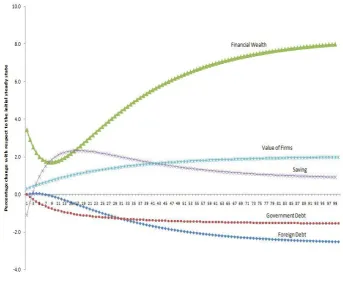
Government debt (-1.54%) is not able to offset the fall in foreign debt (-2.77%). The change

in total assets is positive (see Fig. 6a). This will affect consumption since, in the long-run, the

instability between current wealth and consumption disappears.

Surprisingly, the same type of adjustment is also obtained in the myopic counterpart of FL2.

First, in the short-run, the rate of saving falls for the reason explained above and furthermore

the long-run impact coincides with the forward looking model.

From Figure 6, we see that in both models, savings fall in the initial periods and then rise.

Financial Wealth rises immediately in the first period and then decreases (maintaining

positive change) because foreign debt rises. As soon as the change in foreign debt became

negative, the financial wealth curve rises gently tempered by the fall in Government assets

held by households.

This path analysis confirms that little differences in adjustment and impact exist between

myopic and forward-looking models15. Previous literature has emphasised the incapacity of

the myopic model to produce results that are consistent with rational behaviour (under perfect

foresight). In these experiments instead we demonstrate that both models may reproduce

similar behaviour for the main macroeconomic variables provided effort considerable effort is

devoted to ensure that both models are otherwise comparable in structure.

6.4. Sensitivity analysis.

As we have seen above, the only difference between myopic and forward-looking models is in

the transitional pathway towards a new steady state. In particular, due to the characteristics of

both models, two parameters are able to govern and alter the speed of adjustment: the myopic

15

32

model is highly sensitive to the parameter, , in the investment equation, whilst the inverse of

the constant elasticity of marginal utility, , is the parameter that more than any other alters

the rate at which the new steady state equilibrium is reached in the forward-looking model.

In Figure 7 and 8 we show the differences of changing the parameters and in the myopic

and forward looking models, respectively. As in the preceding simulations, we increase

interregional exports by 10%. Increasing the curve of the proportionate change in the

accumulation rate tends to approach the stable point (zero change) rapidly. Given that capital

stock accumulates over time due to past net investment, a positive shock produces a growth of

GRP generating a large gap between desired and actual K. This causes current net investment

to rise. This rise in investment will increase with the parameter , thereby increasing the

speed of adjustment of the accumulation rate.

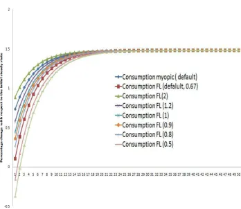
In Figure 8, we report the percentage change of consumption obtained by changing the value

of . Given an intertemporally additive utility function, the Euler equation for expected utility

maximization under rational expectations implies that, by increasing the value of the marginal

utility of consumption and keeping fixed the sacrifice of not consuming (the interest rate), the

cost of reallocating consumption between the present and the future will decrease. So

changing , we modify the cost of reallocating consumption between periods that, according

to the figures, imply that, for a positive shock, consumption will reach the new steady state

faster when is high or its inverse ( ) is low. When is equal to 0.5 and 0.4,

consumption in the initial periods falls due to the fact that households prefer to save in these

33

7. Conclusions

Since regional CGE models are often based on a recursive dynamic structure, the lack of

forward-looking expectations has been stressed as an important drawback of such models

(Partridge and Rickman, 1998; 2011). The focus of this paper is to produce a simple stylized

forward-looking model applicable in a regional context, given that the application of the usual

mechanism and closures applied in national intertemporal CGE models would misrepresent

the adjustment mechanisms that are likely to occur in a region.

The main conclusion is that conventional intertemporal consumer optimization, based on

neoclassical or Fisherian analysis of intertemporal resource allocation, seems to be

inappropriate from a regional point of view. The consumer intertemporal maximization

process not only yields the time path of consumption, but also the time path of savings which

became a function of total financial assets. Thus, not only is the instability between current

income and current consumption, related to the permanent income hypothesis approach,

relevant here, but more emphasis is put on the dynamic path of savings where households are

liable for all the financial needs of the region. In turn, this implies an imposed balance of

payments adjustment mechanism. Furthermore, we question the plausibility, from a regional

point of view, of the imposition of an intertemporal budget constraint where internal and

external debts are made repayable from the private sector. No internal and external debt

sustainability problems occur in a region. Deficit in the current account cannot be seen as

hypothetical surplus in later periods making external debt repayable because there is no

requirement to do so, and foreign debt, especially for declining regions, is the result of capital

subvention supplied by supra-regional institutions, such as a national Government or the

34

government remains committed to the maintenance of the Union. It would, therefore, be a

mistake to allow consumers to take the public deficit into account in their intertemporal

optimization problem, as no taxes will be imposed to cover it and no change in consumption

plans is required. As we noted above, regional policy is an exogenous variable for regions so

no Ricardian equivalence of regional fiscal deficits applies.

We have also argued that some of the objections to myopic models, such as the presumed lack

of capital adjustment in the myopic model and differences in long-run steady state results

between myopic and looking models, cannot be correct. In some articles,

forward-looking models are compared with myopic specifications that preclude any adjustment in

investment and consumption. The usual assumptions are passive investment (or investment

held constant to the base year in real terms) and consumption simply obtained as a fixed share

of current income. In this paper, myopic and forward-looking models that are genuinely

comparable generate the same results in the long-run. The only difference, though of course it

may be a significant one, is in the transitional pathway where consumption and investment

might diverge: perfect foresight agents have rational expectations whilst myopic foresight

agents take decisions according to adaptive expectations and so make no intertemporal

preferences between periods on future profits and incomes. Furthermore, from the sensitivity

analysis we show that the transitional path may be affected by the two types of adjustment

parameters: the speed of adjustment parameter in the myopic model and the intertemporal

elasticity of substitution in the forward-looking model. In the myopic model we have an

adjustment equation in investment while in the forward looking model we have two equations

which influence adjustment speed, one in investment and the other in consumption. The latter

can be interpreted in fact as a flexible accelerator mechanism (like for investment) where the

35

parameter. This is the main structural difference between the myopic and forward looking

models presented in this paper.

It is crucial to appreciate that, independently of the dynamic structure of the model, in the

long-run we obtain identical results for forward-looking and myopic models. This outcome is

much more intuitive than the results obtained in some past studies where the two models’

results differed even in the long-run. Such differences have been attributed to the inability of

the myopic model to produce outcomes consistent with fully rational behaviour due to the

lack of perfect foresight. However, we have shown that comparable regional myopic and

forward-looking CGE models produce equivalent results in the long-run and that the

differences encountered in the past should be attributed to fundamental differences in model

36

APPENDIX A

The mathematical presentation of the model

Prices

( ) (A.1)

( ) _(A.2)

(A.3)

(A.4)

∑ ∑ ̅̅̅

∑ (A.5)

( ( ) ∑ ) _(A.6)

( ) _(A.7)

_{∑ ∑}

_(A.8)

_∑

_(A.9)

( ) ( ) (A.10)

{

[ ] ( ) ( )

( ) ( )

37 ( ) ( ) (A.12) ∑ ∑

∑ ∑ (A.13)

Production technology ( ) (A.14) (A.15) (A.16)

( ) [ ] (A.17)

( ( )

) (A.18)

Trade

_[

] (A.19)

*( ) ( )+ (A.20) _[

] (A.21)

*( ) ( )+ (A.22) ̅ ( ) (A.23) Regional Demand

38 Total Production

(A.25)

Households and other Domestic Institutions

∑( ) (A.26) [ ( ) ( )] ( ₎ (A.27) (A.28) ( ) ∑ ( ) ∑ ∑ ∑ ∑ ∑ ∑ ∑ (A.29)

( ) ∑ ∑ _(A.30)

∑ ∑ ∑

∑

(A.31)

̅̅̅̅̅̅̅ (A.32)

(A.33)

(

)

(A.34)

[ ] (A.35)

39 Government ∑ ̅̅̅̅̅̅̅ ∑ ( ∑ ∑ ∑ ∑ ( ) ∑ ̅̅̅̅ ) (A.37)

[ ] (A.38)

*( ) ( )+ (A.39) Investment Demand

∑ _(A.40)

[ ] (A.41)

[( ) ( )] (A.42) _[

] (A.43)

[( ) ( )] (A.44)

Time path of investment

( ( ) ₎

(A.45) A

40

̇ ( ) (A.47)

( ) ( ) (A.48)

*

+ ( ⁄ ) (A.49)

Factors accumulation

( ) (A.50) A

( ( [ ( ) ( ̅ )] * ( ) ( )+)) _{(A.51) A}

(A.52) A

( ) ∑ _{(A.53) A}

Indirect taxes and subsidies

(A.54) A

∑

(A.55) A

_{(A.56) A}

Total demand for import and current account

∑ ∑ ∑ _{(A.57) A}

∑ ∑ ( ∑ ̅̅̅̅̅̅̅