Nirav dalal, David greenhalgh and Xuerong mao Department of Statistics and Modelling Science
Livingstone Tower, 26 Richmond Street, Glasgow G1 1XH, U.K.
Abstract. We study a mathematical model for the viral dynamics of HIV in an infected individual in the presence of HAART. The paper starts with a literature review and then formulates the basic mathematical model. An expression forR0, the basic reproduction number of the virus under steady state application of HAART, is derived followed by an equilibrium and stability analysis. There is always a disease-free equilibrium (DFE) which is globally asymptotically stable for R0 < 1. Deterministic simulations with realistic parameter values give additional insight into the model behaviour.
We then look at a stochastic version of this model and calculate the proba-bility of extinction of the virus near the DFE if initially there are only a small number of infected cells and infective virus particles. IfR0≤1 then the system will always approach the DFE, whereas ifR0>1 then some simulations will die out whereas others will not. Stochastic simulations suggest that ifR0>1 those which do not die out approach a stochastic quasi-equilibrium consisting of random fluctuations about the non-trivial deterministic equilibrium levels, but the amplitude of these fluctuations is so small that practically the system is at the non-trivial equilibrium. A brief discussion concludes the paper.
1. Introduction. AIDS, or Acquired Immune Deficiency Syndrome, is caused by the Human Immunodeficiency Virus (HIV). First reported in 1981 in the United States, AIDS has become a major worldwide epidemic. By killing or damaging cells of the immune system, HIV progressively destroys the body’s ability to fight infections. Individuals diagnosed with AIDS are susceptible to life-threatening in-fections, which do not cause illness in healthy people [18].
UNAIDS and the WHO estimated that between 36 and 44 million people around the world were living with HIV in December 2004. It was estimated that during 2004, between 4.3 and 6.4 million people were newly infected with HIV and between 2.8 and 3.5 million people with AIDS died. Sub-Saharan Africa remains by far the worst-affected region, with 23.4 million to 28.4 million people living with HIV at the end of 2004. Just under two thirds of all people living with HIV are in sub-Saharan Africa, as are more than three quarters of all women living with HIV [1].
Over the years mathematical models using differential equations have been used to gain an understanding of HIV viral dynamics. The models have evolved over time, including more parameters as we gain more understanding of the disease. One of the
Key words and phrases. HIV, AIDS, HAART, differential equations,R0, equilibrium and sta-bility analysis, deterministic model, stochastic model, probasta-bility of extinction, simulation.
Nirav Dalal was supported by a University of Strathclyde Teaching Assistantship.
benefits of using these models is that it helps us in identifying important parameters and factors which have dominant effect on the development, transmission and spread of the disease. This gives a better understanding for development of treatment strategies and we can draw biologically relevant interpretations.
In this paper we shall study a mathematical model for HIV internal viral dy-namics. HIV viral dynamics is defined as the interaction of the human immune system with HIV. Infection with HIV causes depletion of CD4 T cells, also known as the helper T cells. CD4 T cells play a central role in our immune system. They are involved in protecting against viral, fungal and protozoal infections. These cells normally orchestrate the immune response, signalling other cells in the immune sys-tem to perform their special functions [18]. The depletion of CD4 T cells plays a pivotal role in the degeneration of the immune system in HIV infected individuals.
Two types of HIV infect humans: HIV-1 and HIV-2. HIV-1 is the more vir-ulent and easily transmitted, and is the source of the majority of HIV infections throughout the world. Various methods have been suggested to effectively tackle HIV-1. Early detection and treatment of the disease is one of them [5]. Treatment with a single drug is usually not effective in containing the virus. However individ-uals infected with HIV can be treated with a combination of antiretroviral drugs. This is known as highly active antiretroviral therapy (HAART). HAART works by reducing the HIV viral load in the plasma (usually measured in the blood) to an undetectable level. This delays the onset of the debilitating and ultimately fatal symptoms of AIDS for a very long time, perhaps indefinitely. Nowadays HAART is usually effective but it is expensive, can involve a complicated medication regime including many drugs and has unpleasant side effects. Moreover as HIV mutates rapidly resistance is an increasing problem. Treatment with HAART greatly affects the HIV internal viral dynamics. Viral dynamics under the influence of HAART has been a topic of some major research work recently [2], [4], [6] and [29].
which lead to depletion of HIV-1 virus under HAART. Wu et al. [32] described the reasons for the decay of HIV-1 virus in terms of decay rates. They observed that in persons with moderately advanced HIV-1 infection treated with HAART, there is significant inter-subject variability in the decay rates of HIV-1 virus. These differences were not related to reported or measurable differences in adherence or drug levels. Stafford et al. [25] suggested that cytotoxic T lymphocyte (CTL) destruction of productively infected cells and suppression by CD8+ T cell antiviral factor (CAF) are responsible for lowering the viral load.
The main aim of this paper is to improve existing mathematical models to de-scribe internal HIV-1 viral dynamics in the presence of HAART treatment. We start by formulating the model which includes drug treatment effects into the basic model developed by Bonhoeffer et al. [5] and identify the possible equilibria. The basic reproductive numberR0is a key parameter of the model. We perform a global stability analysis and supplement our theoretical results by numerical simulations of the model. We look at stochastic effects and the probability of extinction in the model. Again our theoretical results are supplemented by numerical simulations. A brief discussion concludes the paper.
2. Model formation. The basic model of Bonhoeffer et al. [5] which describes HIV-1 viral dynamics is given by the following set of differential equations:
˙
x(t) = λ−dx−βxv,
˙
y(t) = βxv−ay,
and v˙(t) = ky−uv.
Here xrepresents the number of uninfected cells,y the number of infected cells andvthe number of virus particles at timet. λis the total rate of production of new uninfected cells per unit time,d, aand uthe per capita death rates of uninfected cells, infected cells and virus particles respectively. Each infected cell produces free virus particles at ratekper unit time. Infected cells are produced from uninfected cells and free virus particles at total rate βxv per unit time. Bonhoefferet al. [5] defined the basic reproductive number
R0= βλk adu
to be the expected number of secondary virus particles produced by a single new virus particle entering a population of uninfected cells at equilibrium with neither infected cells nor virus present. For the above model two equilibria existed. The disease free equilibrium (DFE) was
x= ˆx=λ
d, y= ˆy= 0, v= ˆv= 0
and the endemic equilibrium was given by
x=x∗
= au
βk, y=y ∗
=(R0−1)du
βk , v=v ∗
=(R0−1)d
β .
Nowaket al. [21] also included strains of resistant virus in their model. Analytical approximation for the rate of emergence of resistant virus was studied in this paper. The decline of wild-type virus and the rise of resistant mutant virus in different compartments of the virus populations such as free plasma virus, cells infected with actively replicating virus, long lived infected cells and cells carrying defective provirus was studied. The aim of the paper was to determine the rate of production of plasma virus by cells, half life of infected cells and half life of free plasma virus.
Culshaw and Ruan [9] obtained a restriction on the number of viral particles released per infectious cell in order for infection to be sustained. They also obtained sufficient conditions on the parameters for the stability of the infected steady state. After introducing a time delay into the model which described the time between infection of a CD4 T cell and the emission of viral particles on a cellular level, they derived that the same restriction on the number of viral particles released per infectious cell is required. Stability conditions for the infected steady state in terms of the parameters and independent of the delay were obtained.
Mittleret al. [16] analysed a model for the interaction of HIV-1 virus with target cells and included a time delay between initial infection and the formation of pro-ductively infected cells. They were of the opinion that it was theoretically possible to estimate not only the viral clearance rate and the death rate of productively infected cells, but also the mean and the variance of the infection delay. They obtained an analytical solution for a particular case of delay in which the infec-tion delay conforms to a gamma distribuinfec-tion. They also showed using simulated datasets that the non-linear least-square regression methods used to analyse clini-cal data can, in principle, extract viral dynamic parameters from models in which distributed delays are present.
Huanget al. [12] developed a viral dynamic model to evaluate how time-varying drug exposure and drug susceptibility affected antiviral response. Plasma concen-trations were modelled using a standard pharmacokinetic one-compartment open model with first order absorption and elimination as a function of fixed individual pharmacokinetic parameters and dose times. They observed that poor adherence may result in early viral rebound and a higher set point after treatment failure. Particular patterns of non-adherence affect responses differentially. Also longer se-quences of missed doses increase the chance of treatment failure and accelerate the failure.
There does not seem to be much work which provides analytical conditions for decay in viral load levels. We wish to provide some insight about the parameters and conditions which would have major ramifications on the viral load levels. Tuckwell and Wan [27] analyse a very similar model to ours. However, they do not consider HAART in their model. In addition, we provide a global stability proof and a probabilistic approach for this model.
We propose the following three dimensional model to describe the viral dynamics in the presence of HIV-1 infection and HAART:
˙
x(t) = λ−δx−(1−γ)βxv, (1) ˙
y(t) = (1−γ)βxv−ay, (2) and v˙(t) = (1−η)N ay−uv−(1−γ)βxv (3)
The above model also includes the effect of HAART. HAART is generally a combination of reverse transcriptase inhibitor (RTI) drugs and protease inhibitor (PI) drugs. RTI drugs are designed to prevent the conversion of HIV RNA to DNA in early stages of HIV replication. Thus RTI drugs block conversion of uninfected cells to infected cells. PI drugs are designed to intervene in the last stage of the virus replication cycle to prevent HIV from being properly assembled, and thus cause the newly produced virus to be noninfectious [10]. The treatment effects are accordingly incorporated in the above model.
The variables and parameters in the model are described as follows:
x(t) is the concentration of uninfected cells;
y(t) is the concentration of infected cells;
v(t) is the concentration of virus particles;
(1-γ) is the reverse transcriptase inhibitor drug effect; (1-η) is the protease inhibitor drug effect;
λ is the total rate of production of healthy cells per unit time;
δ is the per capita death rate of healthy cells;
β is the transmission coefficient between uninfected cells and infective virus par-ticles;
a is the per capita death rate of infected cells;
N is the average number of infective virus particles produced by an infected cell in the absence of HAART during its entire infectious lifetime;
and
u is the per capita death rate of infective virus particles.
Note that in the absence of HAART, assuming that the lifetime of an infected cell has an exponential distribution each infected cell is infectious for time (1/a). During its total infectious lifetime it produces (N a)/a=N virus particles.
Also observe that when a single infective virus particle infects a single uninfected cell the virus particle is absorbed into the uninfected cell and effectively dies. Hence the term (1−γ)βxvappears in equation (3) as well as equations (1) and (2). Perelson and Nelson [23] ignored the term (1−γ)βxvin equation (3). The arguments given were first that in examining data from patients with different T-cell counts there was no statistically significant correlation between the T-cell count and the clearance rate. However this may not always be true for all patients in all situations. The second argument given is that if x is approximately constant then the clearance rate can be redefined. As we wish to examine a dynamic model where xmay vary it is better to have this term in the model. Also given that there is a biological justification for this term there is no harm done by including it as the model will be more accurate with this term in than not. One of the models studied by Tuckwell and Wan [27] also includes this term as does a stochastic model by Tuckwell and Le Corfec [26]. However Tuckwell and Le Corfec’s work is relevant only to the early stages of HIV infection.
For our model the equilibrium with no infected cells and no infected virus parti-cles is
(x, y, v) =
λ δ, 0, 0
.
Consider a single infected virus particle entering this equilibrium. Such a particle is infectious for time (u+ (1−γ)βλ
δ)
−1
and during this time infects (1−γ)βλ δ
u+βλ δ(1−γ)
=
(1−γ)βλ
δu+βλ(1−γ) uninfected cells which each survive for average time 1
a and during this
time produce infective virus particles at rate (1−η)N a. Hence the basic reproductive number, defined as the number of secondary infective virus particles caused by a single infective virus particle entering this equilibrium is
R0= βλ(1−γ) (δu+βλ(1−γ))×
(1−η)N a
a =
(1−γ)βλN(1−η) (δu+βλ(1−γ)) .
Note also that a similar argument shows thatR0can be interpreted as the expected number of secondary cells infected by a single infected cell entering the DFE.
Theorem 3.1. The model (1)-(3) describing the viral dynamics has a unique DFE which is globally asymptotically stable forR0<1.
Proof. Clearly our model has a unique DFE x, y, v
= λ δ, 0, 0
. Suppose that
R0 <1. We shall show that (x(t), y(t), v(t))→ λδ,0,0as t→ ∞. We divide the proof into three parts. We first show that limsupx(t)≤λ/δ, then we prove that
y(t), v(t) both tend to zero, then thatx(t)→λ/δ.
From (1) we get
dx(t)
dt ≤λ−δx(t).
Hence we can write
x(t)≤e−δt
x(0) +
Z t
0
λeδsds
which implies that
x(t)≤e−δt
x(0) +λ
δ(1−e −δt
).
Therefore
lim sup
t→∞
x(t)≤ λ
δ.
Next we show thaty andvtend to zero ast→ ∞. Forψ >0 consider d
dt(y+ψv).
d
dt(y(t) +ψv(t)) = [(1−γ)βx(t)v(t)−ay(t)]
+ψ[(1−η)N ay(t)−uv(t)−(1−γ)βx(t)v(t)],
= [(1−ψ)(1−γ)βx(t)−uψ]v(t) + [N a(1−η)ψ−a]y(t).
Now chooseǫ1small enough so that,
1> (1−γ)β(
λ
δ +ǫ1)N(1−η)
(1−γ)β(λ
δ +ǫ1) +u
We can do this because the right hand side of (4) tends toR0 <1 asǫ1→0. Note that with this value ofǫ1
min
1, 1
(1−η)N
> (
λ
δ +ǫ1)(1−γ)β
(1−γ)β(λ
δ +ǫ1) +u
.
So chooseψwith
min
1, 1
(1−η)N
> ψ > (
λ
δ +ǫ1)(1−γ)β
(1−γ)β(λ
δ +ǫ1) +u
.
There existst0 such thatt≥t0 implies thatx(t)≤ λδ +ǫ1. Hence fort≥t0 d
dt(y(t) +ψv(t))≤ −ξ1v(t)−ξ2y(t)
whereξ1=uψ – (1−ψ)(1−γ)β(λδ +ǫ1)>0 andξ2 =a– (1−η)N aψ >0.
Writeπ=y +ψv. Ifπ(0) = 0 theny(0) =v(0) = 0 soy(t) =v(t) = 0 for allt. Ifπ(0)>0 then it is straightforward to show thaty(t) andv(t) are strictly positive fort >0. Ifπ(0)>0 then we can write
d
dtπ(t)≤ −ξ3π(t),
whereξ3= min
ξ1
ψ, ξ2
>0. This implies that
0≤π(t)≤π(t0)e−ξ3(t−t0).
So 0≤y(t)≤π(t0)e−ξ3(t−t0), hencey(t)→ 0 ast → ∞. Similarly v(t)→0 as t → ∞. On the other hand ifπ(0) = 0 then it is straightforward that y(t) andv(t) →0 ast→0.
The final step is to show that x(t) →λ/δ as t → ∞. Now given ǫ2 >0 there existst1such thatǫ2>(1−γ)βv fort≥t1. Hence fort≥t1
dx(t)
dt ≥λ−(δ+ǫ2)x(t). (5)
Multiplying equation (5) bye(δ+ǫ2)t and integrating, it is straightforward to show
that
lim inf
t→∞ x(t)≥ λ δ+ǫ2
.
Butǫ2>0 is arbitrary so lettingǫ2→0 we deduce that lim inft→∞x(t)≥λ
δ. Hence λ
δ ≥lim supt→∞x(t)≥lim inft→∞x(t)≥ λ
δ. Sox(t)→ λ
δ as t→ ∞. The proof is
thus complete.
Tuckwell and Wan [27] analysed a functionally similar model, but without HAART, corresponding toγ=η= 0 in our model. If in our model we define new parameters
is a unique non-trivial equilibrium with infected cells and virus particles present which is LAS. In brief summary for our model forR0 ≤1 there is only the DFE which is LAS for R0 < 1. There is a unique equilibrium with infected cells and virus particles present if and only if R0 > 1 and this equilibrium is LAS when it exists. Moreover the DFE is unstable forR0>1.
Theorem 3.1 extends the results of [27] in that it shows global not local stability of the DFE forR0<1 using completely different mathematical methods than [27]. It also incorporates the effect of HAART and identifiesR0as the basic reproduction number of the virus (alternatively the invasion of infected cells) into the DFE.
4. Deterministic simulations. As we have seen our analytical results suggest the existence of two equilibria for the system (1) - (3). An equilibrium with only uninfected cells present and no infected cells or virus particles always exists and is globally asymptotically stable for R0 ≤1 and is unstable for R0 > 1. A non-trivial equilibrium with uninfected cells, infected cells and virus particles exists for
R0 >1 and is locally stable when it exists. We now use simulations with realistic parameter values to explore the likely behaviour of the model further. The numerical integration package SOLVER was used to integrate the differential equations. We required two sets of parameter values for the simulations. One set was to be used to get a value ofR0<1 and the other one forR0 >1. Hence the parameter values were sourced from different publications so that they would be realistic but need not be significantly altered from the published values.
Our parameter values have all been taken from published literature. λ, β, δ,u,
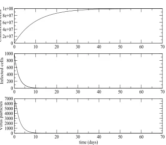
ahave all been taken from [5] andN from [6]. The parameter values for Figure 1 areβ = 1×10⁻¹⁰
day−1
dm3,λ= 107 day−1
dm−3
,N = 100 per cell,γ = 0.2,η
= 0.2,a= 0.5 day−1
,δ= 0.1 day−1
andu= 5 day−1
. The initial values werex(0) = 10000 dm−3
,y(0) = 1000 dm−3
andv(0) = 1000 dm−3
. These parameter values give an R0 value of 0.1278.
As can be seen from Figure1, forR0≤1 the system converges to the equilibrium with only uninfected cells present. The infected cells and the infective virus particles die out and the number of uninfected cells converge toλ/δ. For realistic parameter values even with large initial numbers of cells and virus particles the number of infected cells dropped to 10% of its initial value in around six days. The number of virus particles rises sharply in the beginning but quickly peaks and drops to 10% of its value in approximately nine days. The level of both was virtually zero after only ten days. The number of susceptible cells took slightly longer to reach its very large equilibrium value of 1×10⁸ susceptible cells, but had reached 90% of this value by roughly 25 days and the equilibrium level had virtually been reached after 45 days. The simulations were repeated for a large number of different starting values and in each case the system approached the equilibrium with only uninfected cells present.
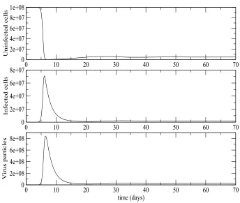
For Figure2the parameter valuesλ,a,uhave been taken from [17] andβ,δare taken from [21]. The value of N remains the same. The values areβ = 1×10⁻⁸
day−1
dm3, λ = 106 day−1
dm−3
, N = 100 per cell, γ = 0.2, η = 0.2, a = 0.5 day−1
,δ= 0.01 day−1
andu= 3 day−1
. These parameter values give anR0value of 16.8421. The initial values were x(0) = 108 dm−3
, y(0) = 0 dm−3
and v(0) = 1 dm−3
. The system converges to the equilibrium where uninfected cells, infected cells and infective virus particles are all present, x → x∗
, y →y∗
and v →v∗
as
0 10 20 30 40 50 60 70 0
2e+07 4e+07 6e+07 8e+07 1e+08
Uninfected cells
0 10 20 30 40 50 60 70
0 200 400 600 800 1000
Infected cells
0 10 20 30 40 50 60 70
time (days) 0
1000 2000 3000 4000 5000 6000 7000
[image:9.612.141.479.109.405.2]Virus particles
Figure 1. Deterministic HIV viral dynamics model in vivo ap-proaches the disease-free equilibrium forR0 <1
of infected cells and virus particles which causes a corresponding sharp decrease in the number of susceptible cells. After this the infected cells and virus particles decline and then tend to their equilibrium values. This equilibrium is reached very quickly after about only 60 days. This simulation was repeated with a variety of different initial conditions and in each case x → x∗
, y → y∗
and v → v∗
as t → ∞suggesting that provided that at least one uninfected cell or one infective virus particle is initially present the system will tend to this equilibrium. In [27] it is shown that for the model without HAART that this equilibrium is LAS when it exists. Our results strengthen these analytical results in two ways:
First our simulations suggest that the equilibrium with infected cells and virus particles is actually globally stable when it exists in the sense that ifR0>1 and at least one infected cell or virus particle is initially present then the system of cells and virus particles will tend to this equilibrium.
0 10 20 30 40 50 60 70 0
2e+07 4e+07 6e+07 8e+07 1e+08
Uninfected cells
0 10 20 30 40 50 60 70
0 2e+07 4e+07 6e+07 8e+07
Infected cells
0 10 20 30 40 50 60 70
time (days) 0
2e+08 4e+08 6e+08 8e+08
[image:10.612.134.478.116.407.2]Virus particles
Figure 2. Deterministic HIV viral dynamics model in vivo ap-proaches the endemic equilibrium forR0 >1
5. Probabilistic approach. While deterministic models have their uses a differ-ent way of looking at the problem of HIV internal viral dynamics would be to use a stochastic model. This can tell us about quantities such as the probability of ex-tinction which deterministic models cannot. A straightforward stochastic analogue of the deterministic model is to assume that the individual stochastic events occur according to a Poisson process with the corresponding rate being the same as in the deterministic model. Further details are given below. Then we can use standard branching process theory to calculate the probability of extinction of the virus.
Wick and Self [31] also use a branching process to model the HIV virus dynamics. The difference between their and our work lies in the assumption of ‘no competition or cooperation’ between the cells and virus particles in Wick and Self. We do not make any such assumption. Also their results are mainly numerical.
When an individual is initially infected with HIV, the usual situation is that they will not be treated with HAART. However there are cases where an exposed individual will be treated with HAART, for example healthcare workers exposed to needlestick injuries [7, 13]. Hence we give the theoretical results with HAART in-cluded and then state them without HAART. In the numerical examples we suppose that HAART is not given, as this is the more usual situation.
the deterministic equilibrium levelλ/δ. This approximation will be valid whilst the number of virus particles and infected cells remains small. This approximation will be valid near the DFE and is a similar approximation to that used to calculate the probability of a major epidemic outbreak in Whittle’s simple stochastic epidemic model [30]. In that paper it is assumed that the number of susceptibles remains constant and the number of infectives is a stochastic birth and death process in order to calculate the probability of a major epidemic outbreak. Once the stochastic process moves away from the DFE this approximation will no longer be valid but it can be used to estimate the probability that the virus and infected cells invade the DFE.
The stochastic model assumes that the probability that each single infected cell dies in [t, t+δt] isaδt+o(δt). The probability that each single virus particle dies in [t, t+δt] isuδt+o(δt). Each virus particle independently infects each susceptible cell in [t, t+δt] with probability (1−γ)βδt+o(δt). When this happens the virus particle is absorbed into the infected cell. Also each infected cell produces a virus particle in [t, t+δt] with probability (1−η)N aδt+o(δt). All infected cells, virus particles, death processes, infections and production of new virus particles are independent.
The translation of the deterministic model into the stochastic model is not a unique process. As virus particles are produced continuously by infected cells we have chosen to assume that each infected cell produces a virus particle in [t, t+δt] with probability (1−η)N aδt+o(δt), and otherwise produces no virus particles in [t, t+δt]. One possible alternative assumption might be to assume that each infected cell simultaneously producesN virus particles in [t, t+δt] with probability (1−η)aδt+o(δt) and otherwise produces no virus particles in [t, t+δt]. This alternative would lead to a qualitatively different solution.
We consider the stochastic model at the equilibrium consisting only of uninfected cells x= λ/δ, y = 0 andv = 0 and consider an initial small infective population of ˜a infective virus particles and ˜b infected cells entering this equilibrium, where ˜a
and ˜b are small. Define q1 = (1 −γ)βλ
(1−γ)βλ+uδ and q2=
(1−η)N
(1−η)N+1. q1 is the probability
that a single infective virus particle at this equilibrium infects a cell before the virus particle ceases to be infective. q2is the probability that a single infected cell at the above equilibrium creates one infective virus particle before it dies. Note that
R0=q1
q2 1−q2
.
Theorem 5.1. Consider a small initial infective population of ˜a infective virus particles and˜b infective cells entering the equilibrium consisting only of uninfected cells. The probability that the population of infective virus particles and infective cells will go extinct without creating a major outbreak is 1 for R0 ≤1 and is
1−q
1q2
q2
˜a1−q 2 q1q2
˜b
for R0>1.
of initially uninfected cells infected by the virus particle before it either loses its infectivity or dies. Then
P(X = 0) = 1−q1, P(X = 1) = q1.
Recall that when a single infective virus particle infects a single uninfected cell the virus particle is absorbed into the uninfected cell and effectively dies. Hence there are only two possible cases that can happen. The probability generating function (p.g.f.) ofX is given by
GX(s) = E(sX),
= 1−q1+q1s.
Now suppose that a single infected cell enters the equilibrium consisting only of uninfected cells. LetY be the number of infected virus particles created before it dies. Then fork= 0, 1, 2, 3, . . .
P(Y =k) =q2k(1−q2). Hence the p.g.f. ofY is
GY(s) =
1−q2 1−q2s
if |s|<1.
Now letZ1denote the number of secondary infective virus particles infected directly by one initial infective virus particle entering the equilibrium consisting only of uninfected cells. The p.g.f. ofZ1 is given by
GZ1(s) = E(s
Z1)
= 1−q1+q1E[sZ1|X1= 1]
= 1−q1+q1
1−q 2 1−q2s
,
whereX1is the number of cells infected by this infective virus particle. The prob-ability of extinction is given by the smallest root ofs=GZ1(s) in [0,1], [8]. Hence
we get
(s−1)((1−q1q2)−q2s) = 0. We obtain the two roots of the above equation as 1 and 1−q1q2
q2 . IfR0 ≤1,
1−q1q2
q2
≥1 and the probability of extinction is 1, whereas if R0 > 1, 1 −q1q2
q2 <1 and the
probability of extinction is 1−q1q2
q2 .
Similarly letZ2 be the number of secondary infective cells produced by a single infective cell entering the DFE.
GZ2(s) = E(s
Z2)
= 1−q2+q2(1−q2)E[sz2|Y1= 1] +q22(1−q2)E[sz2|Y1= 2] +...+q2k(1−q2)E[sz2|Y1=k] +...
= 1−q2+q2(1−q2)(1−q1+q1s) +q22(1−q2)(1−q1+q1s)2 +...+q2k(1−q2)(1−q1+q1s)k+...
= 1−q2 1−q2+q1q2−q1q2s
.
Again solvings=GZ2(s) we get
(s−1)((1−q2)−q1q2s) = 0.
Hence if R0 ≤1, 1q−1qq22 ≥1 and the probability of extinction is 1, whereas ifR0 > 1, 1−q2
q1q2 <1 and the probability of extinction is
1−q2
q1q2.
So the probability of ultimate extinction of a small population of ˜ainfective virus particles and ˜binfected cells, entering the DFE is 1 ifR0 ≤1 and
1−q1q2 q2
˜a
1−q2 q1q2
˜b
ifR0 >1. The proof is thus complete.
In the more practically useful case where HAART is not present the same formula holds whereq1 = βλβλ+δu andq2 = NN+1.
6. Stochastic simulations. Usually newly infected individuals will not be treated with HAART, but occasionally they will be. Hence we keep HAART in theoretical calculations but omit them in the following numerical examples and simulations. We have looked at the simulation of the stochastic system with the same set of parameter values as the deterministic system. The results look very similar.
According to the analytical results in the previous section the probability of extinction of ˜ainitial virus particles and ˜binitial infected cells is 1 for R0 ≤1 and is
1−q
1q2
q2
˜a1−q 2 q1q2
˜b
for R0 > 1. To confirm these observations we carried out stochastic simulations. The simulations assume that the parameter values are the same fixed values as in the deterministic simulations but that events occur at random times given by an exponential distribution with the appropriate rate as described in the detailed description of the stochastic model given in Section 5. Our simulations program was written in FORTRAN and comprehensively verified using detailed output from a large number of runs.
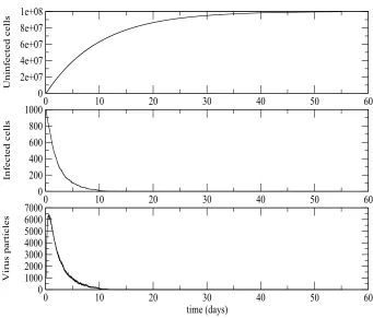
The results obtained were as expected. For those simulations where the number of infected cells and virus particles died out (including those with R0 ≤ 1) the stochastic effects were clearly visible on the trajectories of the number of virus particles and the infected cells, but although stochastic effects were present in the trajectory of uninfected cells, the scaling used meant that this trajectory looked much smoother and more like the deterministic trajectory. Figure3 shows such a simulation with parameters and initial values as in Figure1exceptγ=η = 0. For
R0 >1 we performed simulations with parameters and initial values as in Figure 2 exceptγ =η = 0. Some of these simulations died out and some did not. Those simulations which did not die out tended to the deterministic endemic equilibrium values. Although stochastic effects could be seen if these trajectories were plotted on a very fine scale those trajectories which took off looked practically identical to the deterministic ones in Figure2, if the vertical axis scaling for Figure2 was used.
0 10 20 30 40 50 60 0
2e+07 4e+07 6e+07 8e+07 1e+08
Uninfected cells
0 10 20 30 40 50 60
0 200 400 600 800 1000
Infected cells
0 10 20 30 40 50 60
time (days) 0
1000 2000 3000 4000 5000 6000 7000
[image:14.612.135.476.116.407.2]Virus particles
Figure 3. Stochastic process simulation of HIV viral dynamics model in vivo approaches the disease-free equilibrium forR0<1
Parameter Starting Calculated Prob. 95% Observed No. Set Values of Extinction C.I. Extinctions
1 y= 0,v= 1 0.7600 (733,787) 750
y= 1,v= 0 0.0400 (28,52) 40 2 y= 0,v= 1 0.9657 (954,977) 957
y= 1,v= 0 0.2260 (200,252) 231
Table 1. Calculated extinction probabilities, 95% confidence in-tervals and observed number of 1000 simulations which go extinct for two parameter sets
DFE, that isy = 0,v = 1, and one infected cell entering the stochastic DFE, that is y = 1, v = 0. One set was the values used for Figure 2. The only change was the change in treatment effects, that is γ = η = 0. For the second set of values λ, u were taken from [17], β from [21], δ from [12] and a from [6]. N
remained the same. The values were β = 1×10⁻⁸
day−1
dm3, λ = 106 day−1
dm−3
, γ =η = 0, a = 0.7 day−1
, δ = 0.072 day−1
, u = 3 day−1
[image:14.612.144.468.454.530.2]actual number of simulations which went to extinction lay in the confidence interval. The numbers are given in Table1.
7. Discussion of results. We have discussed an ordinary differential equation model which describes the internal HIV viral dynamics in the presence of treatment such as antiretroviral drugs. We derived an expression for the basic reproductive numberR0 and found that ifR0 was less than or equal to one then the equilibrium with only uninfected cells was the unique equilibrium and was globally asymptoti-cally stable. This paper gives analytical results for the model (1)-(3). Most other work in this area concentrates on obtaining numerical solutions to the problem un-der consiun-deration, which depend on parameter values used [27,31]. Instead we have established some concrete mathematical results for our model as these will be true for all possible parameter values.
Some authors have previously neglected the term (1−γ)βxv in the model in equation (3) as numerically insignificant. This was motivated by statistical studies on viral clearance rates in patients. However this term is biologically realistic as each time that the virus infects a cell it must enter that cell, which means that it cannot infect any more cells. Moreover other authors have also included this term [27,31]. It is of interest to include this term in the model as it is biologically sensible and it may have an effect on the dynamics in some situations and for certain parameter values.
We have also taken a stochastic approach in this paper. The processes of virus replication and the increase of infected cells are highly interdependent processes. Separation of one from the other is not possible. Our branching process approx-imation reflects this interdependence. These results give us the condition for the eradication of the virus and the infected cells in terms of the parameters of the model.
Some recent research has suggested the presence of latent reservoirs in the body in which HIV-1 persists even after the administration of HAART [15,24, 22]. These reservoirs are not biologically significant when the level of virus in the body is high but become significant at low virus loads. They are not important in the deterministic model where viral loads are high. These might possibly be significant when considering the probability of extinction of the virus, however the timescale on which these reservoirs are established is not yet clear.
Acknowledgements. We are grateful to the University of Strathclyde for funding Nirav Dalal by a Graduate Teaching Assistantship.
REFERENCES
[1] AIDS epidemic update, UNAIDS, 2005, www.unaids.org.
[2] S. Bajaria, G. Webb and D. Kirschner,Predicting differential responses to structured treat-ment interruptions during HAART,Bull. Math. Biol.,66(2004), 1093–1118.
[3] H. Banks, D. Bortz and S. Holte,Incorporation of variability into the modelling of viral delays in HIV infection dynamics,Math. Biosci.,183(2003), 63–91.
[4] S. Bonhoeffer, J. Coffin and M. Nowak, Human Immunodeficiency Virus drug therapy and virus load,J. Virol.,71(1997), 3275–3278.
[5] S. Bonhoeffer, G. Shaw, R. May and M. Nowak, Virus dynamics and drug therapy, Proc. Natl. Acad. Sci.,94(1997), 6971–6976.
[6] D. Callaway and A. Perelson, HIV-1 infection and low steady state viral loads,Bull. Math. Biol.,64(2002), 29–64.
[7] D. Cardo, D. Culver, C. Ciesielski, P. Srivastava, R. Marcus, D. Abiteboul, J. Heptonstall, G. Ippolito, F. Lot, P. McKibben and D. Bell,A case-control study of HIV seroconversion in health care workers after percutaneous exposure,N. Engl. J. Med.,337(1997), 1485–1490. [8] D. R. Cox and H. Miller, “The Theory of Stochastic Processes”, Spottiswoode, Ballantyne &
Co. Ltd., London and Colchester, 1965.
[9] R. Culshaw and S. Ruan, A delay-differential equation model of HIV infection of CD4+ T-cells,Math. Biosci.,165(2000), 27–39.
[10] A. Ding and H. Wu,Relationships between antiviral treatment effects and biphasic viral decay rates in modelling HIV dynamics,Math. Biosci.,160(1999), 63–82.
[11] A. Herz, S. Bonhoeffer, R. Anderson, R. May and M. Nowak,Viral dynamics in vivo: limi-tations on estimates of intracellular delay and virus decay,Med. Sci.,93(1996), 7247–7251.
[12] Y. Huang, L. Rosenkranz and H. Wu,Modelling HIV dynamics and antiviral response with consideration of time-varying drug exposures, adherence and phenotypic sensitivity,Math. Biosci.,184(2003), 165–186.
[13] HIV and AIDS: information and guidance in the occupational setting, Health Protection Agency, London, 2006, www.hpa.org.uk
[14] A. Kamina, R. Makuch and H. Zhao,A stochastic modelling of early HIV-1 population dy-namics,Math. Biosci.,170(2001), 187–198.
[15] J. Kulkosky and S. Bray, HAART-persistent HIV-1 latent reservoirs: their origin, mecha-nisms of stability and potential strategies for eradication,Current HIV Research, 4(2006), 199–208.
[16] J. Mittler, B. Sulzer, A. Neumann and A. Perelson,Influence of delayed viral production on viral dynamics in HIV-1 infected patients,Math. Biosci.,152(1998), 143–163.
[17] P. Nelson, J. Murray and A. Perelson, A model of HIV-1 pathogenesis that includes an intracellular delay,Math. Biosci.,163(2000), 201–215.
[18] HIV infection and AIDS, National Institute of Allergy and Infectious Diseases, Bethesda, USA, 2006, www3.niaid.nih.gov.
[19] M. Nowak, R. Anderson, M. Boerlijst, S. Bonhoeffer, R. May and A. McMichael, HIV-1 evolution and disease progression,Science,274(1996), 1008–1010.
[20] M. Nowak, R. Anderson, A. McLean, T. Wolfs, J. Goudsmit and R. May,Antigenic diversity threshold and the development of AIDS,Science,254(1991), 963–969.
[21] M. Nowak, S. Bonhoeffer, G. Shaw and R. May, Antiviral drug treatment: dynamics of resistance in free virus and infected cell populations,J. Theor. Biol.,184(1997), 203–217. [22] T. Pierson, J. McArthur and R. Siliciano,Reservoirs for HIV-1: mechanisms for viral
per-sistence in the presence of antiviral immune responses and antiretroviral therapy,Ann. Rev. Immunol.,18(2000), 665–708.
[23] A. Perelson and P. Nelson,Mathematical analysis of HIV-1 dynamics in vivo,SIAM Review,
41(1999), 3–44.
[24] J. Siliciano and R. Siliciano,A long-term latent reservoir for HIV-1: discovery and clinical implications,J. Antimicr. Chemo.,54(2004), 6–9.
[26] H. Tuckwell and E. Le Corfec,A stochastic model for early HIV-1 population dynamics,J. Theor. Biol.,195(1998), 451–463.
[27] H. Tuckwell and F. Wan,Nature of equilibria and effects of drug treatments in some simple viral population dynamical models,IMA J. Math. Appl. Med. Biol.,17(2000), 311–327. [28] E. Vergu, A. Mallet and J. Golmard,A modelling approach to the impact of HIV mutations
on the immune system,Computers Biol. Med.,35(2005), 1–24.
[29] L. Wein, R. D’Amato and A. Perelson,Mathematical analysis of antiretroviral therapy aimed at HIV-1 eradication or maintenance of low viral loads,J. Theor. Biol.,192(1998), 81–98.
[30] P. Whittle,The outcome of a stochastic epidemic - a note on Bailey’s paper,Biometrika,42
(1955), 116–122.
[31] D. Wick and S. Self,Early HIV infection in vivo: branching-process model for studying timing of immune responses and drug therapy,Math. Biosci.,165(2000), 115–134.
[32] H. Wu, D. Kuritzkes, D. McClernon, H. Kessler, E. Connick, A. Landay, G. Spear, M. Heath-Chiozzi, F. Rousseau, L. Fox, J. Spritzler, J. Leonard and M. Lederman,Characterisation of viral dynamics in human immunodeficiency virus type - 1 infected patients treated with combination antiretroviral therapy: Relationships to host factors, cellular restoration, and virologic end points,J. Inf. Diseases,179(1999), 799–807.