City, University of London Institutional Repository
Citation
:
Braun, V. & Stefanski, B. (2002). Orientifolds and K-theory. Paper presented at the NATO Advanced Study Institute on Progress in String Theory and M-Theory, 24-05-1999 - 05-06-1999, Cargese, France.This is the accepted version of the paper.
This version of the publication may differ from the final published
version.
Permanent repository link:
http://openaccess.city.ac.uk/12559/Link to published version
:
Copyright and reuse:
City Research Online aims to make research
outputs of City, University of London available to a wider audience.
Copyright and Moral Rights remain with the author(s) and/or copyright
holders. URLs from City Research Online may be freely distributed and
linked to.
City Research Online: http://openaccess.city.ac.uk/ publications@city.ac.uk
arXiv:hep-th/0206158v1 18 Jun 2002
hep-th/0206158 HU-EP-02/24 AEI-2002-042
Orientifolds and K–theory
V. Braun,
∗Humboldt Universit¨at zu Berlin, Institut f¨ur Physik Invalidenstrasse 110, D-10115 Berlin, Germany
B. Stefa´
nski, jr.
†Max-Planck-Institut f¨ur Gravitationsphysik, Albert-Einstein Institut Am M¨uhlenberg 1, D-14476 Golm, Germany
May 2002
Abstract
Recently it has been shown that D-branes in orientifolds are not always de-scribed by equivariant Real K–theory. In this paper we define a previously unstudied twisted version of equivariant Real K–theory which gives the D-brane spectrum for such orientifolds. We find that equivariant Real K–theory can be twisted by elements of a generalised group cohomology. This cohomol-ogy classifies all orientifolds just as group cohomolcohomol-ogy classifies all orbifolds. As an example we consider the Ω× I4 orientifolds. We completely determine
the equivariant orthogonal K–theoryKOZZ2(R
p,q) and analyse the twisted
ver-sions. Agreement is found between K–theory and Boundary Confromal Field Theory (BCFT) results for both integrally- and torsion-charged D-branes.
1
Introduction
Brane-anti-brane annihilation [4, 9] is the physical manifestation of the equivalence relations that define K–theory. Lower dimensional D-branes can be thought of as non-trivial tachyon bundles on D ¯brane pairs in Type IIB [6] or non-BPS D9-branes in Type IIA [20]. As such, the spectrum of stable D-D9-branes is classified by K–theory [10, 6, 20]. In this construction D-branes on orbifolds are described by equivariant K–theory while D-branes in Type I and its T-duals correspond to Real K–theory.1
It has been known for some time that certain orbifolds admit discrete torsion [17]. These are classified by the projective representations of the orbifold group G, or equivalently by group cohomology2 H2(G, U
1). The allowed choices give different
closed string backgrounds and hence also different D-brane spectra. It is possible to define twisted equivariant K–theories which describe the D-brane spectrum in orb-ifolds with discrete torsion [6] (see also [13]. We review this construction section 3. It was originally thought that for orientifolds of the form Ω×H, where H is some orbifold group and Ω worldsheet parity, the D-brane spectrum was classified by Real equivariant K–theory [6], KRZZ2×H(X) = KOH(X)3. However, it is
some-times possible to define several distinct orientifolds for a fixed group H; this is somewhat similar to the discrete torsion in orbifolds. Since the closed string spectra differ for such orientifolds, the stable D-branes in these backgrounds are also dis-tinct. It is then clear that KRZZ2×H cannot describe the stable D-branes in all such
backgrounds.
Our work has been motivated by the Ω× I4 orientifolds. These were originally
studied by [11] before the discovery of the significance of D-branes [3]. It was found that there were essentially two such models (in the non-compact case); the massless twisted sector was found to contain either a hypermultiplet or a tensor multiplet. More recently these orientifolds were re-considered in D-brane language. In particular the hypermultiplet model was studied by Gimon and Polchinski [14] and the tensor multiplet model by Blum, Zaffaroni and Dabholkar, Park [16, 15]. We will refer to these models throughout the paper as either hyper, tensor multiplet models or GP, BZDP models.4
Recently all stable D-branes in the two models have been identified using BCFT techniques [1]. As expected the D-brane spectra are quite different, and prelimi-nary results suggested that KRZZ2×ZZ2 corresponds to D-branes in the tensor
mul-tiplet model. It was suggested that D-branes in the hypermulmul-tiplet model should correspond to a twisted version of KRZZ2×ZZ2 in which the anti-linear Ω shouldanti -1Elements of K–theory are pairs of isomorphism classes of complex bundles on a manifold; in
equivariant K–theory a group acts on the bundles with the corresponding map on fibres being linear; Real K–theory or KR–theory is similar to equivariant K–theory but with an element acting anti-linearly (for example by complex conjugation) on the fibres.
2We useU
1 instead ofU(1) for typographical reasons.
3We are using the notation where the involution appears as part of the group in KR-theory.
The equality between the Real and orthogonal K–group follows since the involution is taken to have trivial action on the manifold.
commute with the linear I4 on the fibres. This proposal was made by analogy with
ZZ2×ZZ2 orbifolds. However, it was unclear whether such an object would in fact
form a K–theory. In other words would it satisfy the usual exact sequence and periodicity properties.
The main goal of this paper is to construct twisted KR–theories for all consis-tent orientifolds with fixed groupG. In the process we find a generalisation of group cohomology, so-called group cohomology with local coefficients, which classifies ori-entifolds for a given group G. We will find that, just as the different choices in orbifold theories correspond to projective representations, orientifolds are classified by projective Real representations. Given this classification we obtain twisted KR– theories which give the D-brane spectra of the orientifold theories. In particular we will apply this construction to find the twisted KR–theory which classifies sta-ble D-branes in the GP orientifold. This construction guarantees that the twisted KR–theories satisfy the usual K–theory axioms.
In section 2 we compute KOZZ2(R
p,q) and show that it matches exactly with
the D-brane spectrum of the BZDP model found in [1]. Section 3 contains most of our results. We start by reviewing the construction of twisted equivariant K– theories in section 3.2. We generalise this construction to the Ω× I4 orientifolds
in order to find the KR–theory which corresponds to the hypermultiplet model in section 3.3. We present a general classification of orientifolds in terms of cohomology with local coefficients, and the construction of corresponding twisted KR–theories in section 3.4. In section 4 we give a physical interpretation to the choices allowed for finite abelian orientifolds in terms of phases in front of the different contributions to one-loop partition functions. We conclude and present some open problems in section 5. The paper contains several appendices where some of the technical details of our calculations are presented.
Some work on the classification of orientifolds was carried out in [22]. In [23] cohomology with local coefficients was discussed in a somewhat related, though different, context.
2
Computation of
KO
ZZ2In this section we compute the K–theory relevant to the non-compact BZDP model and show that it agrees exactly with the D-brane spectrum found using BCFT tech-niques. We do this in two different ways; first we use a long exact sequence similar to the one in [8], then we show that the result can be easily obtained by using the connection between Clifford Algebras and K–theory. The former method’s advan-tage is that it identifies which D-branes carry the same charges. This is particularily useful for torsion charged D-branes. The exact sequence method however, becomes quite cumbersome and it is sometimes difficult to disentangle the results.
Following [8] we define a Dp-brane to be a (r, s)-brane if it hass/r+ 1 Neumann directions on which I4 does/does not act and p = r+s. In [1] the D-brane
convenience
ZZ⊕ZZ r= 1,5 and s= 0,4
ZZ r=−1,3 and s= 2
ZZ r= 1,5 and s= 1,2,3 (1)
ZZ2⊕ZZ2 r=−1,0 and s= 0 or r= 3,4 ands = 4
ZZ2 r=−1,0 and s= 1 or r= 3,4 ands = 3.
The first two types of D-branes are BPS and are respectively, the fractional and stuck branes. The third type of integrally charged D-brane are the non-BPS truncated branes; the torsion charged branes are also non-BPS.
In [1] it was suggested thatKOZZ2 should be the K–theory which classifies such
D-branes. In particular, in the non-compact theory, an (r, s)-brane should correspond to
KOZZ2(R
4−s,5−r), (2)
where the bundles are taken to have compact support and ZZ2 acts as
(x1, . . . , x4−s, x5−s, . . . , x9−s−r)7→(−x1, . . . ,−x4−s, x5−s, . . . , x9−s−r). (3)
As a first step towards computing such KO-theories we note that they are 8-periodic
KOZZ2(R
p,q) = KO
ZZ2(R
p+8,q) =KO
ZZ2(R
p,q+8), (4)
and that for p= 0 the group action is trivial and we get immediately
KOZZ2(R
0,q) =KO(Rq)⊗RO(
ZZ2), (5)
where the real representation ring of ZZ2 isRO(ZZ2) =ZZ⊕ZZ. Therefore
q 0 1 2 3 4 5 6 7
KO(Rq) ZZ ZZ
2 ZZ2 0 ZZ 0 0 0
KOZZ2(R
0,q)
ZZ⊕ZZ ZZ2⊕ZZ2 ZZ2⊕ZZ2 0 ZZ⊕ZZ 0 0 0
(6)
which agrees with the spectrum of (5−q,4)-branes.
The other K–groups can be computed using long exact sequences. For general manifolds Y ⊂X our K–theory satisfies the usual long exact sequence
· · · →KO−1
ZZ2(Y)→KOZZ2(X, Y)→KOZZ2(X)→KOZZ2(Y)→. . . , (7)
which, due to periodicity is 24–cyclic. With
this becomes5
· · · →KO−1(Rp+q)→KO
ZZ2(R
p+1,q)→KO
ZZ2(R
p,q)→KO(Rp+q)→ · · · . (9)
We have used the fact that D1,0 is contractible (in anZZ
2–equivariant way)
KOZZ2(D
1,0×Rp,q) =KO
ZZ2(R
p,q) (10)
and that the ZZ2–action is free on S1,0 ={+1} ∪ {−1}.
KOZZ2(S
1,0×Rp,q) =KO(Rp+q). (11)
Given KO∗
ZZ2(R
p,q) and KO∗
(Rp+q) it is then possible to deduce KO∗
ZZ2(R
p+1,q).
Further, for p= 0 the forgetting map
KOZZ2(R
0,q)→KO(Rq) (12)
is onto. From this it is easy to show that
q 0 1 2 3 4 5 6 7
KOZZ2(R
1,q) ZZ ZZ
2 ZZ2 0 ZZ 0 0 0 (13)
which is in agreement with the (5−q,3)-brane spectrum in equation (1). Further-more the maps
KOZZ2(R
1,s)→KO
ZZ2(R
0,s) (14)
are one-to-one, indicting that the ZZ2 charge of the (r,3)-brane is the same as (part
of the) charge of the (r,4)-brane forr = 3,4. One may continue in this way, however it becomes increasingly difficult to solve the extension ambiguities.
Instead we will now use the connection between K–theory and Clifford algebras to compute the K–groups. One finds that [2]
KOZZ2(R
p,q) =KO(0,p+1)(Rq). (15)
In Appendix A we defineKO(m,n)(X) and prove the above result. The above formula
is useful since the object on the right hand side is purely algebraic and is well known [26]:
KOZZ2(R
p,q) =
q=7 0 0 0 0 0 0 0 0
q=6 0 0 ZZ ZZ2 ZZ2⊕ZZ2 ZZ2 ZZ 0
q=5 0 0 0 ZZ2 ZZ2⊕ZZ2 ZZ2 0 0
q=4 ZZ⊕ZZ ZZ ZZ ZZ ZZ⊕ZZ ZZ ZZ ZZ
q=3 0 0 0 0 0 0 0 0
q=2 ZZ2⊕ZZ2 ZZ2 ZZ 0 0 0 ZZ ZZ2
q=1 ZZ2⊕ZZ2 ZZ2 0 0 0 0 0 ZZ2
q=0 ZZ⊕ZZ
O
O
/
/
ZZ ZZ ZZ ZZ⊕ZZ ZZ ZZ ZZ
p=0 p=1 p=2 p=3 p=4 p=5 p=6 p=7
(16)
5Sm,nandDm,n are the unit sphere and disk inRm,nwith inherited
Comparing with equation (1) we see exact agreement between the spectrum of BZDP D-branes and the K–theory predictions.
3
Twisting in equivariant K–theory
In this section we construct a K–theory which describes the D-brane spectrum of the GP orientifold. Comparing the D-brane spectrum of the GP model (see appendix C) with the results of the previous section it is clear that this is not described byKOZZ2.
Instead, we argue that D-branes in the hyper model are described by a twisted K– theory KR[D8]
ZZ2×ZZ2. We present a unified picture of twisting equivariant K–theories,
which allows for twists involving linear as well as anti-linear group elements. We begin the section by discussing such twisting in the case of K[D8]
ZZ2×ZZ2 which gives the
D-brane spectrum of the ZZ2×ZZ2 orbifold with discrete torsion. In the following
subsection we obtain KR[D8]
ZZ2×ZZ2. The construction is then generalised to describe
generic non-compact orientifolds; as a by-product we show that these are classified by a cohomology group H2 ∗,Ue
1
much in the same way as orbifolds are classified by H2(∗, U
1) [17].
3.1
Twisting for ordinary orbifolds
Let us quickly review how group cohomology enters twists of ordinary K–theory, that is how discrete torsion alters the K–groups. This section is not strictly necessary for the understanding of the rest of the paper, we only want to recall how the twisted K–theory appearing in the analysis of WZW models [36, 37] is related to discrete torsion and projective representations.
If spacetime X is a bona fide manifold, i.e. not an orbifold, then the twist is caused by a nontrivial B-field. In such a background D–branes no longer carry ordinary gauge bundles but “twisted bundles”, where the transition functions hij do
not close [6, 38, 39]. Instead there is a U1 valued function on triple overlaps such
that
hjkh
−1
ik hij =gijk. (17)
Ignoring torsion in H3(X,ZZ) the twist class corresponds to the de Rahm class of
the flux dB via the well-known identity6
[gijk]∈H2 X;U1
∼
−→H3(X;ZZ)∋[dB]. (18)
Mathematically this corresponds to the statement that you can twist ordinary K– theory K(X) by H2 X;U
1
.
Now orbifold string theory onX/Gis reallyG-equivariant theory on the manifold
X. The relevant K–theory is equivariant K–theoryKG(X) and it can be twisted by
classes in the equivariant cohomology group H2
G X;U1
. Now for general (topolog-ically nontrivial) manifolds X all possible twists may be difficult to determine, but
6U
there is a rather well-understood subclass of twists. These come from pullbacks via the projection π:X →pt from H2
G(pt;U1), that is we are interested in the image
π∗
HG2(pt;U1)
⊂HG2 X;U1
. (19)
The advantage of this subclass is that
HG2(pt;U1) =H2(BG;U1) =H2(G, U1), (20)
whereBGis the base space of the classifying spaceEG. The connection to group co-homology yields an interpretation of spacetime twists as projective representations. Motivated by this we now turn to the classification of projective representations.
3.2
Twisted equivariant complex K–theory
For an orbifold group G which admits projective representations (see below) there are several orbifolds consistent with modular invariance [17]. Typically it is possible to define the action of some generator gi in several different ways on a gj-twisted
sector (i 6= j) giving distinct closed string backgrounds. As a result the D-brane spectrum is distinct in each of the orbifolds. G-equivariant K–theory will then describe the D-brane spectrum in the orbifold without discrete torsion, and one has to define twisted versions ofKGwhich describe the D-brane spectrum of the various
orbifolds with torsion. These twisted K–theories are the Grothendieck group of isomorphism classes of bundles with a projective representation of G on the fibres rather than a proper representation.
Recall that a projective representation of a finite groupG is a representation of the central extension ofGbyU1such thatU1 acts by multiplication with a phase. In
other words a projective representation ofGis a choice ofH such that the following sequence is exact
1→U1 i
−→H −→π G→1 (21)
and U1 is in the centre of H.
Choose a section s:G→H such that π◦s= idG. This is always possible since
π is surjective, but in general s will not be a group homomorphism. The failure to be a group homomorphism
s(g1)s(g2) =c(g1, g2)s(g1g2) (22)
defines a function c:G×G→U1. An ordinary representation of H ρ :H → GLn
defines a projective representation of G via γ = ρ◦s : G → GLn, which will be a
“representation up to phases”. In particular, as is familiar to physicists, it satisfies
γ(g1)γ(g2) =c(g1, g2)γ(g1g2). (23)
Requiring that s or γ be associative restrictsc to satisfy
c(g1, g2)
1
c(g1, g2g3)
c(g1g2, g3)
1
c(g2, g3)
In group cohomology language the left hand side defines the coboundary of a two-cocycle and the above equality says that c is coclosed. Further, given a function
G → U1 (by abuse of notation also called c) we can replace s(g) → c(g)s(g) and
then
s(g1)s(g2) =c(g1, g2)s(g1g2) → s(g1)s(g2) =
c(g1g2)
c(g1)c(g2)
c(g1, g2)s(g1g2). (25)
Hence 2-cocycles that differ by
c(g1)c(g1g2)
−1
c(g2) (26)
correspond to the same extension. The above defines a coboundary of a 1-cochain in group cohomology, and therefore we identify
projective representations ofG
=
central extensions 1→ U1 →H →G→1
= H2 G, U1
.
(27)
A twisted G-equivariant vector bundle is a vector bundle with the group G acting by a projective representation.7 Such bundles form a semigroup under the Whitney
sum, and as usual we can define the Grothendieck group KG[H](X) corresponding to
H ∈ H2 G, U
1
. By equation ((27)) any representation of H is either a proper or a projective representation of G. Succinctly, at the level of K-theory this implies a decomposition
KH(X) =KG(X)⊕KG[H](X). (28)
Since both KG and KH satisfy the usual K–theory properties, such as periodicity
and long exact sequences, then so does KG[H].
As an example consider G = ZZ2 × ZZ2 with generators g1, g2. The D-brane
spectrum of these orbifolds is well known [19, 24]. The groupsKZZ2×ZZ2 for Euclidean
space have been computed and have been found to agree with the D-brane spectrum of the orbifold with no discrete torsion [19]. Since
H2 ZZ2×ZZ2, U1
=ZZ2 (29)
there is one nontrivial projective representation given by the following choice of normalised (meaning s(1) = 1) section:
s(g1)s(g2) = −s(g1g2) =−s(g2)s(g1), s(g1)2 =s(g2)2 = 1. (30)
This projective representation is a representation of the group D8
D8 =
n
σ, γ1, γ2
γ1γ2 =σγ2γ1, γ12 =γ22 =σ2 = 1
o
(31)
7One of us (BS) learnt about this approach to twisted equivariant K–theory from Burt Totaro
where the generator σ is represented by −1 (and acts trivially on the base space
X). Since D8 irreducible representations decompose into projective and ordinary
representations of ZZ2 ×ZZ2 the K–theory of D8 splits as in equation (28):
KD8(X) =KZZ2×ZZ2(X)⊕K
[D8]
ZZ2×ZZ2(X). (32)
The above equation not only shows thatK[D8]
ZZ2×ZZ2 is well defined but is also useful in
computing twisted equivariant K–groups if the groups act trivially on the base (e.g.
X = pt). As usual we have
KGi(pt) =Ki(pt)⊗R[G], (33)
where the representation rings are [35]
R[D8] =ZZ⊕5, R[ZZ2×ZZ2] =ZZ⊕4. (34)
Then equation (32) yields8
Ki(pt)⊗ZZ5 =Ki(pt)⊗ZZ4
⊕K[D8],i
ZZ2×ZZ2(pt)
⇒ K[D8],i
ZZ2×ZZ2(pt) =K
i(pt) =
0 iodd
ZZ ieven (35)
in agreement with the presence of (2k1 + 1; 2k2,2k3,2k4)-branes in the Type IIB
orbifold with discrete torsion [24].
We note that the twisted K–theory defined by representations of Q8, the unit
quaternions,
Q8 =
n
σ, γ1, γ2
γ1γ2 =σγ2γ1, γ12 =γ22 =σ, σ2 = 1
o
(36)
is the same as the D8-twisted K–theory defined above. This is because the two
yield projective representations of ZZ2×ZZ2 that differ by a coboundary (c.f.
equa-tion (29)). This will be in contrast to the case of Real K–theory, as we will see in the next section.
3.3
Defining
KR
[D8]ZZ2×ZZ2
In this subsection we wish to extend the construction of twisted equivariant K– groups to KR–groups. Following the above discussion it seems clear that D-branes in the GP model are described by a K–theory of bundles on which g acts linearly,
τ acts anti-linearly, and the two anti-commute. Consider then D8-equivariant KR
theory in which g and σ act linearly and τ acts anti-linearly. Such K–theories have
8Below, and throughtout the text, we write equalities between different K-groups. These are
meant to indicate that there is an isomorphism between such groups. It should be however, understood that such equalities need not map generators to generators; for example presently in the equality between K[D8],i
ZZ2×ZZ2(pt) andK
i(pt) the generator of the twisted group gets mapped to
been considered in the mathematical literature [27, 32]. Any representation9 of
D8 is either a representation of ZZ2 ×ZZ2 or a projective representation (τ and g
anti-commute). At the level of K–theory this is
KRD8(X) = KRZZ2×ZZ2(X)⊕KR
[D8]
ZZ2×ZZ2(X). (37)
As in the previous section this guarantees that KR[D8]
ZZ2×ZZ2 is a K–theory.
In order to confirm that KR[D8]
ZZ2×ZZ2 is the K–theory which describes D-branes
in the hypermultiplet model we shall compute it on R0,i, on which ZZ
2 ×ZZ2 acts
trivially. There are three irreducible representations ofD8 withτ acting anti-linearly
(we denote complex conjugation by δ)
g 1 σ g τ
r1(g) 1
1 1 1◦δ
r2(g) 1
1 −1 1◦δ
r3(g)
1 0 0 1
−1 0 0 −1
0 i
−i 0
1 0 0 1
◦δ
(38)
The analogue of equation (33) in KR–theory is [32]
KRG(X) =
AG⊗KO(X)
⊕BG⊗K(X)
⊕CG⊗KSp(X)
, (39)
where the representation ring of G decomposes as
R[G] =AG⊕BG⊕CG (40)
according to commuting field R,C,H. Both 1-dimensional representations have commuting field R and one can easily show that the commuting field for r3 is C.10
Then equations (37) and (39) gives
KRZZ2×ZZ2(X) =KO(X)⊕KO(X)
KRD8(X) =KO(X)⊕KO(X)⊕K(X)
⇒ KR[D8]
ZZ2×ZZ2(X) = K(X) (42)
In particular for X =Ri with trivial group action we find that
KR[D8],i
ZZ2×ZZ2(pt) =K
i(pt) =
0 i odd
ZZ i even (43)
which is in agreement with the presence of ZZ charged (2k+1,4)-branes in the GP model [1] (see also (80)).
9We use the word representation somewhat loosely here as γ(τ) acts anti-linearly on a vector
space. Really we are talking about Real representations; we shall give more precise definitions in the next section.
10The (complex) matrices commuting with r 3 are
F3def= R
1 0 0 1 +R 0 1
−1 0
≃C (41)
Repeating the above construction for the unit quaternionsQ8to obtainKR[Q
8]
ZZ2×ZZ2
one comes across a surprise. As we show in appendix C
KR[Q8]
ZZ2×ZZ2(pt) =KSpZZ2(pt)6=KR
[D8]
ZZ2×ZZ2(pt). (44)
This stems from the fact that projective representations ofZZ2×ZZ2 which are
repre-sentations ofD8(withτ acting anti-linearly) are not equivalent modulo coboundaries
to those of Q8. Clearly then we need a generalisation of H2(G, U1) to classify all
inequivalent such representations.
3.4
Classification of Orientifolds
In the previous subsection we have shown that projective representations of ZZ2 ×
ZZ2 in which one of the generators acts anti-linearly differ significantly from linear
projective representations. In this subsection we will generalise group cohomology to take into account such differences. This will allow us to classify the analogue of discrete torsion in orientifolds, and to obtain suitable twistings of KR–theory which will describe D-branes in such models.
An orientifold group has linear and anti-linear elements. To keep track of which act linearly and which anti-linearly we will use the notion of an augmented group, that is a group together with a homomorphism ǫ :G→ZZ2. A Real representation
of Gon some complex vector spaceV associates to eachg ∈Ga linear or antilinear map V →V depending on whether ǫ(g) = +1 or ǫ(g) =−1.
As before we want G to act “up to phases”. By the same reasoning as in sec-tion 3.2 this means we have to find an extension
1 //U1 i //H π //
ǫ′def=ǫ◦π AA A A A A A
A G
/
/
ǫ
1
ZZ2
(45)
However, there are two important differences compared to equation (21):
• G is now an augmented group, andH inherits an augmentation ǫ′
.
• The extension is no longer central: complex conjugation acts on the U1.
Since anti-linear elements act by complex conjugation on U1-phases, conditions (24)
and (26) have to be modified. In particular the differentials of 1- and 2-cochains are
dc(g1, g2) =c(g1)
1
c(g1g2)
g1◦c(g2) (46a)
dc(g1, g2, g3) =c(g1, g2)
1
c(g1, g2g3)
c(g1g2, g3)
1
g1◦c(g2, g3)
(46b)
where
g◦c(h)def=
(
c(h) if ǫ(g) = 1
Mathematically this is well-known as group cohomology with local coefficients (by abuse of notation again denoted H∗
(G, F)) where the group in the first slot, G, acts on the second, F.11 We will use Ue
1 to denote the “U1 with action on it”. Then
H2G,Ue1
(48)
classifies all inequivalent non-compact G orientifolds. Further a non-trivial projec-tive Real representation ofGgives a Real representation of some groupHand hence an element [H] ∈ H2 G,Ue
1
, just as in equation (27). This may be used to con-struct KR[GH], the K–theory which gives the D-brane spectrum of this particular G
orientifold
KRH(X) = KRG(X)⊕KR[GH](X). (49)
In appendix D we compute the cohomology of the most general finite abelian orientifold group, in particular we find
H2ZZ2 ×ZZ2,Ue1
=ZZ2⊕ZZ2. (50)
As we have seen the projective Real representations given by [Q8] and [D8] are
in-equivalent, and so they can be taken as the generators ofH2 ZZ
2×ZZ2,Ue1
. From the explicit 2-cocycles (see appendix B) we can then identify the following inequivalent projective Real representations of ZZ2×ZZ2,
[(ZZ2)3] : g2 = 1, τ2 = 1, gτ =τ g ,
[D8] : g2 = 1, τ2 = 1, gτ =−τ g ,
[Q8] : g2 =−1, τ2 =−1, gτ =−τ g ,
[ZZ2×ZZ4] : g2 =−1, τ2 =−1, gτ =τ g .
(51)
As a result there are four inequivalent twisted KRZZ2×ZZ2 theories. Those twisted
by (ZZ2)3[] (i.e. untwisted) and [D8] give the D-brane spectrum of the tensor and
hyper models. Space-time filling branes in the [Q8] twisted theory are classified
by KSpZZ2. This describes D-branes in the I4 orbifold of the Type I theory with
Sp gauge group, and a twsited sector tensor multiplet. Similarly then the theory twisted by [ZZ2×ZZ4] gives the D-brane spectrum of the I4 orbifold of the Type I
theory with Sp gauge group, and a twisted sector hypermultiplet. In appendix C, generalising [1], we have computed the D-brane spectrum of both theSporientifolds, and (partially) matched it with the corresponding twisted KR–theories.
As a further example to illustrate the construction consider orientifolding Type IIB by Ω. One easily shows that
H2ZZ2,Ue1
=ZZ2. (52)
11 In [33] it was noted that this possibility so far did not appear in the physics literature, but
The untwisted KR–theory is simply
KRZZ2(X) =KO(X), (53)
which indeed describes D-branes in the Type I SO theory. The KR–theory twisted by the generator of H2 ZZ
2,Ue1
is
KR[ZZ4]
ZZ2 (X) = KSp(X), (54)
which gives the D-brane spectrum of the Type I Sp theory. This example was also discussed in [34].
4
Physical interpretation
In the previous section we have shown that for an orientifold group G there are
H2(G,Ue
1) different models, and that given a particular such orientifold [H] ∈
H2(G,Ue
1) we can construct the K–theoryKRG[H]which classifies the stable D-branes
in it. In appendix D we have computedH2(G,Ue
1) for the most general finite abelian
orientifold group. In this section we analyse the various one-loop partition functions in the orientifold and identify the places where a choice of phase is allowed without spoiling the properties of such partition functions. We will show that the physically acceptable choices are isomorphic to elements of H2(G,Ue
1).
The most general finite abelian orientifold groupGis generated by anti-linear el-ements t1,· · · , ta and linear elementss1,· · · , sb. This is equivalent to the orientifold
group generated by t, g1,· · · , gn, h1,· · · , hm, where t is the only anti-linear element
(of even order), thegi are linear even-order elements and thehi are linear odd-order
elements.12 In appendix D we show that
H2(G,Ue1) =
n
⊕ i=1ZZ2
⊕ZZ2⊕
n
⊕ i<j=1ZZ2
=ZZ⊕2n(n+1)/2+1. (55)
We will interpret each of the three terms in the middle of the above equation as coming from phase choices in front of the various one-loop partition functions.
Consider first the torus amplitude. In an orbifold given two generators K and
L of order k and l it is possible to choose a phase ωp = exp(2πip/gcd(k, l)) with
p= 1,· · · ,gcd(k, l) in front of the torus amplitude
ωpTrK Le−tHc . (56)
The trace is taken over the K-twisted sector with L inserted and Hc is the closed
string Hamiltonian. This phase effectively changes the action of Lon theK-twisted groundstate. Then for K and L to remain order k and l respectively, various other parts of the torus amplitude will change their phases. For example we will have
ω−pTrK Le−tHc . (57)
12This equivalence holds as< t
1,· · ·, ta >generates the same group as< t1, t1t2· · ·, t1ta>and
Recently it has been shown [22] that orbifolds with discrete torsion different from±1 cannot be consistently projected by Ω. The argument also applies to more general anti-linear elements t. From it we see that the ⊕n
i<j=1ZZ2 factor in equation (55)
comes from the orbifold discrete torsion which is allowed for an orientifold back-ground. Hence, as in [17], the phase in front of the g1-twisted sector amplitude with
g2 inserted is proportional to c(g1, g2)/c(g2, g1) where c∈ H2 G,Ue1
. In particular it is worth noting that there is no consistent discrete torsion between two odd-order elements.
An anti-linear order two elementτ ∈Ggives rise to an Orientifold plane coupling to the untwisted sectors.13 As is well known the overall sign of the normalisation
of this crosscap state can be freely chosen; for example this choice of sign in the Ω orientifold of Type IIB gives the Type I theory with SO or Sp gauge groups. It is easy to show that for anti-linear τ ∈ G with τ2 = 1 c(τ, τ) = ±114 and as a result
the corresponding M¨obius strip amplitude has the phase
c(τ, τ)Tr τ e−tHo , (60)
whereHo is the open string Hamiltonian. Such phase choice is possible for t∈Gas
well as for tgi ∈G if the order of these elements is 4k+ 2.
For an anti-linear element τ ∈Gof order 4k the difference of signs between the Klein bottle amplitudes
Trτ2 τ e−tHc and Trτ2 τ2k+1e−tHc (61)
gives two different, consistent models (see for example [41])15. With a bit more
work it is possible to show as above that c(τ, τ)/c(τ2k+1, τ2k+1) = ±1, and this is
the cocycle contribution which keeps track of this choice. We can now explain the appearance of ⊕ni=1 ZZ2
⊕ZZ2 in equation (55). Each
element t, tg1,· · · , tgn is even-order and anti-linear. If its order is 4k + 2 then
we may choose a phase proportional to c(tgi, tgi) which governs the overall sign
of the orientifold plane. On the other hand if it is of order 4k we may choose a sign proportional to c(tgi, tgi)/c((tgi)2k+1,(tgi)2k+1) as described in the previous
paragraph. Either way each t, tg1,· · · , tgn gives rise to a ZZ2 choice. In total this
reproduces the ⊕n i=1ZZ2
⊕ZZ2 factor in equation (55).
Finally, it is possible to convince oneself that there are no other phase choices that we can make consistently. For example in the Ω×ZZ3 orientifold we may only
choose the overall sign of the O9-planes. One might think that the natural phase
13For example ΩIn gives rise to an O(9−n)-plane described by the crosscap state
|O(9−n)i=|C(9−n)iNS-NS +|C(9−n)iR-R . (58)
14Withg
1=g2=g3=τ the cocycle condition (46b) becomes
c(τ, τ)c(1, τ) =c(τ,1)¯c(τ, τ). (59) Sincec(1, τ) =c(τ,1) = 1 the above impliesc(τ, τ) = ¯c(τ, τ) =±1.
e2πi/3 could appear in the twisted sector crosscaps. However, the square of this
phase appears in the untwisted sector Klein bottle with g (the generator of ZZ3) or
g2 inserted. The action of g on the untwisted sector is unique and hence we cannot
pick up a phase here. This argument can be extended to show that indeed the above choices are the only ones which are consistent.
5
Conclusion and Outlook
We have computedKRZZ2×ZZ2(R
p,q) which classifies D-branes in theI
4×Ω orientifold
with twisted sector tensor multiplet, and found complete agreement with the BCFT results [1]. We have also constructed a twisted version of this KR–theory relevant to the model with twisted sector hypermultiplet. In the process we have identified a type of cohomology which classifies orientifolds, in a similar way to the classification of orbifolds by the second group cohomology [17]. We have presented a unified approach towards twisting complex and Real K–theories. This procedure allows for the straightforward identification of K–groups relevant to orbifolds and orientifolds with discrete torsion. We have found places in the various one-loop diagrams where
±1 phases may be introduced and have shown that for finite abelian orientifold groups this freedom is precisely described by cohomology with local coefficients.
In compact orientifolds it was shown that not all possible orientifolds are al-lowed [42]. In particular there are global conditions which only allow configurations with 8k hypermultiplets and 32−8k tensor multiplets (k = 0,1,2,3,4). It would be very interesting to show that these results follow from the cohomology we have presented here. Perturbative orientifolds with the same orientifold group differ from one another by the presence of discrete background Bµν fields, it should be possible
to make this connection more precisely. In particular it would be interesting to un-derstand better how the ten-dimensional Type I SO andSptheories are connected. Finally, it should prove instructive to try to obtain the classification by cohomology with local coefficients from considering ‘modular transformations’ of two-loop non-oriented diagrams, in a similar way to the discrete torsion results found in [17]. We hope to return to these results in the near future [44].
Acknowledgements
A
Clifford algebras and
K
p,qReview of Clifford algebras
Our notation is based on [27, 25] but without the category–theoretic language, see also [2]. For completeness we review it here:
Definition 1. The Clifford algebraCp,qR is the real algebra generated byγ1, . . . , γp+q
subject to the relations
γiγj =−γjγi ∀ i6=j
γi2 =−1 ∀ i∈ {1, . . . , p}
γ2i = +1 ∀ i∈ {p+ 1, . . . , p+q}
(62)
The Clifford algebras enjoy the following well–known properties:
CpR+n,q+n≃Mat2n C
p,q
R
(63a)
CpR+8,q ≃C
p,q+8
R ≃Mat16 C
p,q
R
(63b)
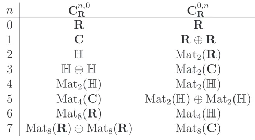
So there are only finitely many cases to determine, the complete list is in table 1 (see e.g. [28]). Note that the notation also reflects the multiplication in the Clifford
alge-n Cn,R0 C
0,n
R
0 R R
1 C R⊕R
2 H Mat2(R)
3 H⊕H Mat2(C)
4 Mat2(H) Mat2(H)
5 Mat4(C) Mat2(H)⊕Mat2(H)
6 Mat8(R) Mat4(H)
[image:17.612.173.422.375.512.2]7 Mat8(R)⊕Mat8(R) Mat8(C)
Table 1: List of Clifford algebras
bra; For example C0R,1 is the algebra of pairs (x1, x2)∈R⊕R with componentwise
multiplication. Especially (1,0)(0,1) = (0,0).
Now a Cp,qR vector bundle is an ordinary vector bundle E with an action of the
Clifford algebra, that is a map ρ : Cp,qR → End(E). With other words the Clifford
algebra acts on the fibres of E via ρ(γi) :Ex →Ex.
You can addCp,qR bundles in the usual way, so by the usual Grothendiek
construc-tion we get K–theory for bundles with Cp,qR action, denoted KO(p,q)(X). But those
are not very interesting groups: A real bundle with R, C or H action is simply a real, complex or quaternionic bundle and the semigroups of bundles and semigroups of bundles with some matrix algebra action are isomorphic16. Furthermore if the
16This can be seen as follows: By the Mat
n(R) action one can decompose a bundle E in the
sum ofnisomorphic bundlesE=⊕n
i=1Ei. With the correspondenceE↔E1we can identify the
Clifford algebra is the sum of two orthogonal pieces (like R⊕R) we can use the actionρ(1,0),ρ(0,1) of the projectors (1,0) and (0,1) to decompose the bundle into the sum of two independent bundles. So from the last column of table 1 we can simply read of the K–groups in table 2.
KO(0,0)(X) = KO(X) KO(0,1)(X) =KO(X)⊕KO(X)
KO(0,2)(X) = KO(X) KO(0,3)(X) =K(X)
KO(0,4)(X) = KSp(X) KO(0,5)(X) =KSp(X)⊕KSp(X)
KO(0,6)(X) = KSp(X) KO(0,7)(X) =K(X)
Table 2: List of the C0R,q K–groups
More interesting are the groupsKOp,q(X) which fit into the long exact sequence
associated to the “restriction of scalars” r:Cp,qR+1 →C
p,q
R :
KO(p,q+1)(X×R)→r KO(p,q)(X×R)→KOp,q(X)→KO(p,q+1)(X)→r KO(p,q)(X)
(64)
So KOp,q(X) is represented by formal differences of
Cp,qR+1 vector bundles that are
the same if considered as Cp,qR vector bundles. Another way to think about that is
the following: A Cp,qR+1 vector bundle structure on a given C
p,q
R vector bundle E is
equivalent to a gradation on E:
Definition 2. A gradation on aCp,qR vector bundle(E, ρ)∈Vect
p,q
R is an involution
η∈ End(E) such that η2 = 1 and ηρ(γ
i) =−ρ(γi)η ∀i∈ {1, . . . , p+q}
The group KOp,q(X) is then the group generated by triples (E, η
1, η2) subject
to the relations
• (E, η1, η2) + (F, ξ1, ξ2) = (E⊕F, η1⊕ξ1, η2⊕ξ2)
• (E, η1, η2) = 0 if η1 is homotopic to η2 within the gradations of E.
From these properties one can deduce the following:
• (E, η1, η2) + (E, η2, η1) = 0 • E ≃E′
, η1 ≃η1′, η2 ≃η2′ ⇒ (E, η1, η2) = (E′, η1′, η
′
2)∈KOp,q(X)
i.e. KOp,q(X) depends only on the isomorphism classes of bundle and
grada-tions.
• (E, η1, η2) + (E, η2, η3) = (E, η1, η3)
• Every element of KOp,q(X) can be represented by a single triple.
One can recover ordinary KO-theory from KOp,q(X) via the following:
KO0,0(X) = KO(X) (65)
To see this let (E, η1, η2)∈KO0,0(X). Then η1, η2 are just involutions, they do not
have to satisfy anything else. Maybe after adding the trivial triple (X×Rn,1 n,1n)
one can simultaneously diagonalise both involutions and then cancel the eigenspaces with the same eigenvalue. You are left with a difference of triples (E1,−1k,1k)−
Computation of KOZZ2
All the KOZZ2(R
p,q) groups can be determined by using the connection between K–
theory and Clifford algebras. The basic idea is to use the following result of [27] (for notation see appendix A)
Theorem 1. Let G be a compact Lie group, V a G vector space with a positive definite form (i.e. the generated Clifford algebra is C(V) with all γ2
i = +1) and X
a Real G space. Then
KRVG(X) =KRG(X×V) (66)
This reduces the calculation to one where the base space is a point, and then use a trick to absorb the ZZ2 action in the Clifford algebra.
Of course we want to compute KO and not KR, so we want the real version of the above theorem. So let the Real involution act trivially on every space (that is
G, X and V), then
KOVG(X) =KOG(X×V) (67)
The correspondence between KO↔KRclasses is as usual by complexification (→) resp. taking the subbundle invariant under the complex conjugation (←). Note that for the V–action to be well–defined on the real subbundle we need that the complex conjugation acts trivially on Clifford algebra, i.e. on V.
So letV =Rp,0 and let it generate
C(V) =C0R,p. We then get
KOZZ2(R
p,q) =KO
ZZ2(R
0,q×V) =KOV
ZZ2(R
0,q) (68)
Now we have to reinterpret KOV
ZZ2(X) for some ZZ2–invariant space X. Its elements
are tuples (E, g, ρ;η1, η2) where
• E is a real vector bundle over the base space X.
• g :E →E is an involution that acts trivially on the base (i.e. g ∈End(E)).
• g acts also on the Clifford algebra via g :V →V, v7→ −v.
• An action of the Clifford algebra ρ:C0R,p →End(E)
• Two gradations η1, η2.
This data is equivalent to the following:
• A real vector bundle E over the base space X.
• An action of the Clifford algebra ˜ρ:C0R,p+1 →End(E) defined by
˜
ρ(γi) =
ρ(γi) ∀ i∈ {1, . . . , p}
• η˜1,η˜2∈ End(E) that commute with theC0R,p+1 action defined by
˜
ηi =gηi (70)
Since the ˜ηi commute with the Clifford algebra action this is not KO0,p+1(X); The
gradations and the Clifford algebra can rather be treated independently.
However we can think of ˜ηi as two gradations of someC0R,0 =Raction on (E, ρ).
But then by the analog of equation (65) for “bundles with C0R,p+1 action” instead of
ordinary bundles we find that
KOVZZ2(X) =KO
(0,p+1)(X) (71)
B
Understanding
H
2(
ZZ
2×
ZZ
2,
U
e
1)
Following (appendix D) we have determined H2 ZZ
2×ZZ2,Ue1
=ZZ2×ZZ2, so there
are four different twists by which KRZZ2×ZZ2 can be twisted. One of them is just
untwistedKRZZ2×ZZ2, and one of them isKR
[D8]
ZZ2×ZZ2 of section 3.3. We discuss the
re-maining two twists in some detail presently. This appendix is designed to familiarise the reader with group cohomology with coefficients in Ue1.
The 2-torsion part of H2 ZZ
2 ×ZZ2,Ue1
comes from H2(ZZ
2 ×ZZ2,ZZ2) via the
ZZ2 →Ue1 →Ue1 coefficient long exact sequence. The advantage of this description is
twofold: First there is no complex conjugation action onZZ2 and second determining
H2(ZZ
2×ZZ2,ZZ2) is a finite combinatorial problem. Elementary calculation shows
that
H2(ZZ2×ZZ2,ZZ2) =ZZ2×ZZ2×ZZ2 (72)
corresponds to the extensions
0→ZZ2 → D8 or Q8 orZZ2×ZZ4 orZZ32 →ZZ2×ZZ2 →0 (73)
Let us denote the linear generator with g and the anti-linear one with τ, so that
D8 =
n
σ, τ, ggτ =στ g, g2 =τ2 =σ2 = 1o
Q8 =
n
σ, τ, ggτ =στ g, g2 =τ2 =σ, σ2 = 1o (74)
where the projection toZZ2×ZZ2is always by puttingσ = 1. To determine the
corre-sponding group 2-cocycle we choose sectionss(γ1) =τ, s(γ2) =g, ands(γ1γ2) =τ g.
For example
cD8(−,−) =
c(τ, τ) c(g, τ) c(τ g, τ)
c(τ, g) c(g, g) c(τ g, g)
c(τ, τ g) c(g, τ g) c(τ g, τ g)
=
+ − −
+ + + + − −
There are altogether 16 closed 2-cocycles and one coboundary
c(τ) =c(g) =−1, c(τ g) = +1 ⇒ dc(−,−) =h+−− −+− − −+
i
(76)
so the quotient consists of the 8 cohomology classes ZZ2×ZZ2×ZZ2.
Now we are really interested in their image inH2 ZZ
2×ZZ2,Ue1
, for that we have to mod out the additional coboundary
c(τ) =c(g) = i, c(τ g) = +1 ⇒ dc(−,−) =h++− −− −
+ + +
i
(77)
Therefore the 4 classes are
cZZ3
2(−,−) =
h+ + +
+ + + + + +
i
≃h+−− −+− − −+
i
≃h++− −− −
+ + +
i
≃h+ + +− −+
− −+
i
(78a)
cD8(−,−) =
h+− −
+ + +
+− −
i
≃h+ + +−+− −+−
i
≃h+ + ++− −
+− −
i
≃h+− −− −+ −+−
i
(78b)
cQ8(−,−) =
h− −+
+− −
−+−
i
≃h−− −+−+
+− −
i
≃h−+ + ++−
−+−
i
≃h− −−++−
+− −
i
(78c)
cZZ2×ZZ4(−,−) =
h−+−
+− −
− −+
i
≃h− −− −++ + + +
i
≃h− −+ + ++
− −+
i
≃h−−++−−
+ + +
i
(78d)
The new twist classes corresponding to the 2-cocyclescQ8,cZZ2×ZZ4 have c(τ, τ) =−1,
so the corresponding projective representation of ZZ2 ×ZZ2 is one with τ2 =−1.
C
The D-brane spectrum and K–groups for
Ω
× I
4orientifolds
In [1] the D-brane spectrum of the hyper and tensor multiplet models was computed using BCFT techniques. It is possible to generalise these results to the two Ω× I4
Sp orientifolds. The four theories differ from one another by the overall choice of sign in front of the O9- and O5-plane crosscaps.
Theory O9 O5
So tensor / BZDP − +
So hyper / GP − −
Sp tensor + −
Sp hyper + +
(79)
We note in particular that the Sp tensor model is T-dual (performing T-duality along all four internal directions) to the BZDP model. Since the Sp model comes from an orbifold of a non-supersymmetric theory (Type I withSpgauge group) this puts in doubt the possibility of the BZDP model being supersymmetric17. Like the
GP model the Sp hyper model is T-dual to itself.
It is then straightforward to repeat the computation of [1] to obtain the D-brane spectrum of the two Sp theories. We list below the D-brane spectrum of all four models.18
Theory ZZ⊕ZZ BPS ZZ non-BPS ZZ ZZ2⊕ZZ2 ZZ2
SO tensor / BZDP (1,5; 0,4) (1,3; 2) (1,5; 1,2,3) (−1,0; 0),(3,4; 4) (−1,0; 1),(3,4,3)
SO hyper / GP (−1,3; 2) (1,5; 0,4) (−1,3; 0,1,3,4) (5,2) (5; 1,3
Sptensor (1,5; 0,4) (−1,3; 2) (1,5; 1,2,3) (−1,0; 4),(3,4; 0) (−1,0; 3),(3,4; 1)
Sphyper (−1,3; 2) (1,5; 0,4) (−1,3; 0,1,3,4) (1,2; 2) (1,2; 1,3) (80)
One can compute the various twisted KR theories for R0,q using equation (32).
We only have to determine the Real irreducible representations of the groups. For
Q8 we find (again δ denotes complex conjugation)
g 1 σ g τ
r1(g) 1
1 1 1◦δ
r2(g) 1
1 −1 1◦δ
r3(g)
1 0 0 1
−1 0 0 −1
i 0
0 i
0 1
−1 0
◦δ
r4(g)
1 0 0 1
−1 0 0 −1
−i 0 0 −i
0 1
−1 0
◦δ
(81)
One can easily check that the commuting field for r3, r4 is H, therefore by
equa-tion (39)
KR[Q8],i
ZZ2×ZZ2(pt) =KSp
i(pt)⊕KSpi(pt) =KSpi
ZZ2(pt). (82)
Explicitly we have for R0,q with trivial group action
q 0 1 2 3 4 5 6 7
KSpZZ(R0,q) ZZ⊕ZZ 0 0 0 ZZ⊕ZZ ZZ2⊕ZZ2 ZZ2⊕ZZ2 0
(83)
which agrees with the spectrum of D(5−i,4)-branes in equation (80). Finally, take for the group defining the remaining twist [D8Q8]
D8Q8 =
n
σ, τ, g
gτ =τ g, g2 =τ2 =σ, σ2 = 1o (84)
Its Real irreducible representations are
g 1 σ g τ
r1(g) 1
1 1 1◦τ
r2(g) 1
1 −1 1◦τ
r3(g)
1 0 0 1
−1 0 0 −1
0 1
−1 0
0 1
−1 0
◦τ
(85)
18Entries in equation (80) are of the form (r
1,· · ·, rm;s1,· · ·, sn) to indicate that all D(ri, sj
The only higher-dimensional Real representation r3 has commuting field C, and
therefore
KR[D8Q8],i
ZZ2×ZZ2(pt) =K
i(pt) (86)
This matches with the spectrum of D(5−i,4)-branes in equation (80).
D
Cohomology for general abelian groups
In this section we want to compute the cohomology group H2 G,Ue 1
for all finite abelian groups
G=ZZ2r×
n
× i=1ZZki
× ×m j=1ZZℓj
ki even, ℓj odd (87)
where the augmentation ǫ: G → ZZ2 is −1 on the generator of the first factor and
+1 on the other generators. By redefinition of the generators we can always assume that only one generator acts anti-linearly.
Now it is technically easier to use the ZZe → IRe → Ue1 coefficient long exact
sequence (for finite groups Hi(G,IR) = 0)e
0→H2G,Ue1
∼
−→H3G,ZZe→0 (88)
and actually compute H3 G,ZZe. Then the computation naturally splits into two
steps:
1. Compute the group cohomology for general cyclic groups
2. Put the cohomology groups of the factors together via the K¨unneth theorem
The former is standard [43]
Theorem 2. Let G = ZZk be any cyclic group and M an arbitrary ZZ[G] module.
Then the cohomology groups are
Hi(G, M) =
kerN i odd
cokerN =MG/NM i >0 even
MG i= 0
(89)
where19 N :M
G →MG is the norm map N(m) =Pki=1gi(m).
19The invariants and coinvariants ofM are defined as
MG= {m∈M|g(m) =m} and MG= M
In particular we have
i= 0 i= 1 i= 2 i= 3 i= 4
Hi ZZ
2r,ZZe
0 ZZ2 0 ZZ2 0
Hi ZZ
kj,ZZ
ZZ 0 ZZkj 0 ZZkj
Hi ZZ
ℓj,ZZ
ZZ 0 ZZℓj 0 ZZℓj
(91)
To assemble the cohomology groups of G from the factors we then need the
Theorem 3 (K¨unneth theorem). Let G1, G2 be groups (such that resolutions
are finitely generated, e.g. finite groups). Furthermore let M1 be a ZZ[G1] module
and M2 a ZZ[G2] module such that either M1 or M2 is ZZ-free. Then there is a split
exact sequence
0−→ M p+q=i
Hp(G
1, M1)⊗Hq(G2, M2)
−→Hi(G
1×G2, M1⊗M2)−→
−→ M
p+q=i+1
TorHp(G1, M1), Hq(G2, M2)
−→0 (92)
Since in our case the cohomology groupsH∗
(ZZ2r,ZZe) are only 2-torsion and the
above theorem implies that the sequence splits we see20 that the cohomology of the
general abelian group G is only 2-torsion. This matches the physical expectation that only ±1∈ U1 twists are allowed (see section 4).
Moreover the odd order factors in G do not contribute: viewed as a ZZ-module equation we have ZZ2⊗ZZℓ = 0 = Tor(ZZ2,ZZℓ) forℓ odd we see that
H∗
ZZ2r×ZZℓ,ZZe
=H∗
ZZ2r,ZZe
ℓ odd (93)
so we only have to consider the cyclic subgroups of even order. For those the relevant cohomology groups can be summarised as follows:
Theorem 4. For Gn def
= ZZ2r⊕
n
⊕ i=1ZZki
we have
i= 0 i= 1 i= 2 i= 3
Hi G
n,ZZe
0 ZZ2 ZZn2 ZZ
1+n(n+1)/2 2
(94)
Proof. Induction: It is correct for n = 0 (equation (91)). Then by the K¨unneth theorem
H0 Gn+1,ZZe
=0 (95a)
H1 Gn+1,ZZe
=ZZ2 (95b)
H2 Gn+1,ZZe
=ZZ2⊕ZZn2 =ZZn2+1 (95c)
H3 G
n+1,ZZe
=ZZ21+n(n+1)/2⊕ZZ2⊕ZZn2 =ZZ
1+(n+1)(n+2)/2
2 (95d)
⊓ ⊔
20Recall that Tor(
Putting everything together we have learnt that
H2
ZZ2r⊕
n ⊕ i=1ZZki
⊕ ⊕m j=1ZZℓj
,Ue1
=ZZ21+n(n+1)/2 ki even, ℓj odd. (96)
References
[1] N. Quiroz and B. Stefa´nski, jr, Dirichlet branes on orientifolds, [hep-th/0110041].
[2] V. Braun, K–Theory and Exceptional Holonomy in String Theory, PhD thesis, to appear.
[3] J. Polchinski, Dirichlet-Branes and Ramond-Ramond Charges, Phys. Rev. Lett.
75 (1995) 4724, [hep-th/9510017].
[4] A. Sen, Stable non-BPS states in string theory, JHEP 9806 (1998) 007, [hep-th/9803194];
A. Sen, Stable non-BPS bound states of BPS D-branes, JHEP9808(1998) 010, [hep-th/9805019];
A. Sen, Tachyon condensation on the brane antibrane system, JHEP 9808
(1998) 012, [hep-th/9805170];
A. Sen, SO(32) spinors of type I and other solitons on brane-antibrane pair, JHEP 9809 (1998) 023, [hep-th/9808141];
A. Sen, Type I D-particle and its interactions, JHEP 9810 (1998) 021, [hep-th/9809111].
A. Sen, BPS D-branes on non-supersymmetric cycles, JHEP 9812 (1998) 021 [hep-th/9812031].
[5] O. Bergman and M. R. Gaberdiel, Stable non-BPS D-particles, Phys. Lett. B
441 (1998) 133, [hep-th/9806155].
[6] E. Witten, D-branes and K–theory, JHEP9812 (1998) 019, [hep-th/9810188]. [7] M. Frau, L. Gallot, A. Lerda and P. Strigazzi,Stable non-BPS D-branes in type
I string theory, Nucl. Phys. B 564 (2000) 60, [hep-th/9903123].
[8] M. R. Gaberdiel and B. Stefa´nski, jr., Dirichlet branes on orbifolds, Nucl. Phys. B 578 (2000) 58, [hep-th/9910109].
[9] M. Srednicki, IIB or not IIB, JHEP 9808 (1998) 005, [hep-th/9807138]. [10] R. Minasian and G. Moore,K–theory and Ramond-Ramond charge, JHEP9711
(1997) 002, [hep-th/9710230].
[12] C. Angelantonj and A. Sagnotti, Open strings, arXiv:hep-th/0204089.
[13] J. Gomis, D-branes on orbifolds with discrete torsion and topological obstruc-tion, JHEP 0005 (2000) 006 [arXiv:hep-th/0001200].
[14] E. G. Gimon and J. Polchinski, Consistency Conditions for Orientifolds and D-Manifolds, Phys. Rev. D 54 (1996) 1667, [hep-th/9601038].
[15] A. Dabholkar and J. Park, A note on orientifolds and F-theory, Phys. Lett. B
394 (1997) 302, [hep-th/9607041].
[16] J. D. Blum and A. Zaffaroni, An orientifold from F theory, Phys. Lett. B 387
(1996) 71, [hep-th/9607019].
[17] C. Vafa, Modular Invariance And Discrete Torsion On Orbifolds, Nucl. Phys. B 273 (1986) 592.
[18] C. Vafa and E. Witten, On orbifolds with discrete torsion, J. Geom. Phys. 15
(1995) 189, [hep-th/9409188].
M. R. Douglas, D-branes and discrete torsion, [hep-th/9807235].
M. R. Douglas and B. Fiol,D-branes and discrete torsion. II, [hep-th/9903031].
[19] B. Stefa´nski, jr., Dirichlet branes on a Calabi-Yau three-fold orbifold, Nucl. Phys. B 589 (2000) 292, [hep-th/0005153].
[20] P. Horava,Type IIA D-branes, K-theory, and matrix theory, Adv. Theor. Math. Phys. 2 (1999) 1373 [arXiv:hep-th/9812135].
[21] O. Bergman, E. G. Gimon and P. Horava, Brane transfer operations and T-duality of non-BPS states, JHEP 9904 (1999) 010, [hep-th/9902160].
[22] M. Klein and R. Rabadan,Orientifolds with discrete torsion, JHEP0007(2000) 040 [arXiv:hep-th/0002103].
[23] O. Bergman, E. G. Gimon and S. Sugimoto, Orientifolds, RR torsion, and K-theory, JHEP 0105 (2001) 047 [arXiv:hep-th/0103183].
[24] M. R. Gaberdiel, Discrete torsion orbifolds and D-branes, JHEP 0011 (2000) 026, [hep-th/0008230].
[25] M. Karoubi, Alg`ebres de Clifford et K–th´eorie, Ann. Scient. ´Ec. Norm. Sup.,
4(1) (1968) 161–270.
[26] M. Karoubi, K–Theory, Springer, 1978.
[28] M. F. Atiyah, R. Bott, and A. Shapiro,Clifford modules, Topology,3(1)(1964) 3–38.
[29] B. Totaro, Private Communications.
[30] M. F. Atiyah, Private Communications.
[31] G. B. Segal, Private Communications.
[32] M. F. Atiyah and G. B. Segal, Equivariant K-theory and completion, J. Diff. Geom. 3 (1969) 1–18.
[33] E. R. Sharpe, Discrete Torsion and Gerbes I, [hep-th/9909108].
[34] S. Gukov, K–theory, Reality, and Orientifolds, Commun. Math. Phys. 210
(2000) 621–639, [hep-th/9901042].
[35] J. P. Serre, Linear representations of finite groups, Springer-Verlag, 1996.
[36] A. Alekseev and V. Schomerus, arXiv:hep-th/0007096.
[37] S. Fredenhagen and V. Schomerus, JHEP 0104 (2001) 007 [arXiv:hep-th/0012164].
[38] D. S. Freed, E. Witten, Anomalies in String Theory with D-Branes, [hep-th/9907189].
[39] P. Bouwknegt, V. Mathai,D-branes, B-fields and twisted K-theory, JHEP0003
(2000) 007, [hep-th/0002023].
[40] A. Kapustin, D-branes in a topologically nontrivial B-field, Adv. Theor. Math. Phys. 4 (2000) 127 [arXiv:hep-th/9909089].
[41] R. Rabadan and A. M. Uranga,Type IIB orientifolds without untwisted tadpoles, and non-BPS D-branes, JHEP 0101 (2001) 029 [arXiv:hep-th/0009135]. [42] J. Polchinski, Tensors from K3 orientifolds, Phys. Rev. D 55 (1997) 6423
[arXiv:hep-th/9606165].
[43] K. S. Brown, Cohomology of Groups, Springer-Verlag, 1982.