Effect of the integration method on the accuracy and computational efficiency of free energy calculations using thermodynamic integration

For Review. Confidential - ACS

Effect of Integration Method on the Accuracy

and Computational Efficiency of Free Energy

Calculations Using Thermodynamic Integration

Miguel Jorge1*, Nuno M. Garrido1, António J. Queimada1, Ioannis G. Economou2,3, Eugénia A. Macedo1

1. LSRE Laboratory of Separation and Reaction Engineering, Departamento de Engenharia

Química, Faculdade de Engenharia, Universidade do Porto, Rua do Dr. Roberto Frias, 4200 -

465 Porto, Portugal

2. Molecular Thermodynamics and Modeling of Materials Laboratory, Institute of Physical

Chemistry, National Center for Scientific Research “Demokritos”, GR-15310 Aghia Paraskevi

Attikis, Greece

3. The Petroleum Institute, Department of Chemical Engineering, PO Box 2533, Abu Dhabi,

United Arab Emirates

*

Author to whom all correspondence should be addressed at: [email protected]

Revised Manuscript for submission to

Journal of Chemical Theory and Computation.

For Review. Confidential - ACS

Abstract

Although calculations of free energy using molecular dynamics simulations have

gained significant importance in the chemical and biochemical fields, they still remain quite computationally intensive. Furthermore, when using thermodynamic integration,

numerical evaluation of the integral of the Hamiltonian with respect to the coupling parameter may introduce unwanted errors in the free energy. In this paper, we compare the performance of two numerical integration techniques – the trapezoidal and

Simpson’s rules – and propose a new method, based on the analytic integration of physically-based fitting functions that are able to accurately describe the behavior of the

data. We develop and test our methodology by performing detailed studies on two prototype systems, hydrated methane and hydrated methanol, and treat Lennard-Jones and electrostatic contributions separately. We conclude that the widely used trapezoidal

rule may introduce systematic errors in the calculation, but these errors are reduced if Simpson’s rule is employed, at least for the electrostatic component. Furthermore, by

fitting thermodynamic integration data we are able to obtain precise free energy estimates using significantly fewer data points (5 intermediate states for the electrostatic component and 11 for the Lennard-Jones term), thus significantly decreasing the

associated computational cost. Our method and improved protocol were successfully validated by computing the free energy of more complex systems – hydration of

2-methylbutanol and of 4-nitrophenol – thus paving the way for widespread use in solvation free energy calculations of drug molecules.

Keywords: free energy, thermodynamic integration, molecular simulation, solvation, non-linear regression;

For Review. Confidential - ACS

1. Introduction

Calculation of free energies is extremely important for a wide spectrum of

technological areas, perhaps most notably in the pharmaceutical industry, where solvation free energy estimates are essential to predict, for example, drug solubility and

protein-ligand binding energies 1, 2. Thus, computational methods that are able to predict accurate solvation free energy values can bring tremendous advances in drug design methodologies. With recent improvements in computer power and algorithms,

molecular simulation-based free energy calculations are being performed in a more routine way (as an example, a recent paper by Mobley et al. calculated the hydration

free energy of 504 compounds using molecular simulation3). Nevertheless, we have not yet reached a stage where these methods are predictive enough for practical use4. A major stumbling block is the fact that the parameterization of most molecular force

fields does not take free energy data into account (a notable exception being the recent parameterizations of the GROMOS force field5), which is understandable given that

such calculations are still much more computationally demanding than calculations of bulk fluid properties and phase equilibria. There is thus a pressing need to make free energy calculation methods as fast as possible. Furthermore, such calculations must be

very precise – if the error intrinsic to the calculation method is small (high precision), any differences between simulation and experiment can be confidently attributed to

inaccuracies in the molecular model, which can then be appropriately refined. The problem is that precision and speed do not normally come hand-in-hand, and in practice one must find an appropriate balance between the two. In this work, we explore

different integration methods in an attempt to improve both the precision and the speed of free energy calculations using Thermodynamic Integration (TI) of molecular

simulation data.

For Review. Confidential - ACS

TI, originally proposed by Kirkwood6, is the most widely used, and perhaps most robust, method for computing solvation free energies of complex solutes (for a

review of other methods and a more detailed description of TI, the reader is referred, for example, to the recent book by Chipot and Pohorille7). The TI method considers a

transition between two generic well-defined states, an initial reference state (state 0) and

a final target state (state 1), described by the Hamiltonians H_{0 and}

1

H _{, respectively. A}

coupling parameter, λ, is added to the Hamiltonian, H

(

_{p q}, ;λ

)

_{, where p is the linear}

momentum and q the atomic position, and used to describe the transition between the

end-points: H

(

_{p q}, ; 0

)

→H

(

_{p q}, ;1

)

_{. Considering several discrete and independent} λ

values between 0 and 1, equilibrium averages can be used to evaluate derivatives of the

free energy with respect to λ. One then integrates the derivatives of the free energy

along a continuous path connecting the initial and final states in order to obtain the energy difference between them:

(

)

1 0

, ,

G d

λ

λ λ λ

∂ ∆ =

∂

∫

H p q

(1)

where the angular brackets indicate an ensemble average at a particular value of λ.

Equation (1) is exact, but suffers from two possible sources of error: i) the statistical

error in the ensemble average of the Hamiltonian derivative at each value of λ, and ii)

the error associated to the integration of the curve. The first error can be reduced, in

principle, by increasing the length of each individual simulation. The second type of error is normally addressed by increasing the number of intermediate points. Indeed, it has been concluded that the precision of the TI methodology depends mostly on the

For Review. Confidential - ACS

smoothness of the ∂H ∂λ _vs. λ _plot 8_{. As a rule of thumb, it was suggested that the free}

energy difference between two consecutive points (λ and λ + ∆λ) should be less than 2

kcal/mol 9. If we deal with a system containing high energy barriers, the number of

intermediate steps may become considerably large and the associated computational cost too high. Here, we analyze in detail the impact of the choice of integration method

and the number of intermediate points on the precision of the free energy estimate. The trapezoidal rule is by far the most widely used method to numerically

evaluate the integral in equation (1) when estimating ∆G via TI. A notable exception is the use of Gauss-Legendre integration in the work of Smith et al.10 The trapezoidal rule

performs a linear interpolation between successive points, and can thus suffer from systematic errors if the underlying function is very far from linearity (which is indeed

the case for most practical calculations). An alternative to reduce such deviations is to use a more elaborate integration method, such as the Simpson rule. However, to our knowledge, this has not been previously explored in free energy calculations. Another

option would be to fit the entire data set to an appropriate functional form, and then perform the integration of this function analytically. This idea has been applied before

by Swope and Andersen11 where average solute – water interactions in the hydration of

inert gases were fitted as a function of the coupling parameter and by Hummer and

co-workers in the context of charging free energies 12. Recently, while this manuscript was

being prepared, Shyu and Ytreberg 13 have demonstrated that the use of polynomial functions to fit simulation data can significantly increase the precision of the free energy

estimates over the trapezoidal rule, without requiring additional simulations. However, they have examined only very simple prototype systems, with an analytical solution to the free energy and smooth monotonous curves. As we will show below, simple

For Review. Confidential - ACS

polynomial functions are not the best choice to describe the curves that arise in hydration free energy calculations, even for small solutes.

In the present work, we compare the performance of two numerical integration techniques – the trapezoidal rule and Simpson’s rule – in the calculation of free energies

from TI. Furthermore, we develop a physically-based fitting function that is able to accurately describe the variation of the Hamiltonian derivative with respect to the coupling parameter. By fitting this function to the simulation data, we are able to obtain

precise free energies using significantly fewer intermediate points, thus decreasing the associated computational cost. We carry out our detailed study for two prototype

systems, methane and methanol in water, which represent realistic solutes (both polar and apolar) and solvent, but are simple enough to allow for long simulations to be

performed at a very large number of intermediate values of λ, an essential requisite to

assess the validity of our procedure. We then apply our methodology to the solvation of two larger and more complex molecules, namely 2-methylbutanol and 4-nitrophenol, in order to demonstrate its applicability in realistic free energy calculations. In the

following section, we present a detailed description of the simulation methods, while the integration methods and the development of the fitting function are explained in

Section 3. Section 4 presents the results of our study followed by the main conclusions in Section 5.

2. Computational Details

Molecular dynamics (MD) simulations were performed using the GROMACS

simulation suite14. Hydrated systems consisted of one solute molecule (methane, methanol, methylbutanol or 4-nitrophenol) represented by the OPLS-AA15 force field and 500 water molecules represented by the SPC/E16 model (parameters for the models

For Review. Confidential - ACS

are provided in Tables S1-S4 of the Supporting Information). Covalent bonds involving hydrogen atoms were constrained with the LINCS17 algorithm while the water geometry

was fixed with the SETTLE18 algorithm. For efficiency reasons 19 we have used the reaction-field method, originally proposed by Lee et al.20, with a cut-off distance of 1

nm and a dielectric permittivity of 80, to account for long-range electrostatic interactions. The remaining cut-off radii used were 1 nm for the short-range neighbor list and a 0.8-0.9 nm switched cut-off for the LJ interactions. We have applied long

range corrections for energy and pressure as suggested in the work of Shirts el al.8. Simulations were performed using periodic boundary conditions in all directions.

Newton’s equations of motion for all species were integrated using the leap-frog dynamic algorithm21 with a time step of 2 fs. Langevin stochastic dynamics22 was used to control the temperature, with a frictional constant of 1 ps-1, while for constant

pressure runs the Berendsen barostat23, with a time constant of 0.5 ps and an isothermal compressibility of 4.5×10-5 bar-1, was used to enforce pressure coupling.

The TI method makes use of a thermodynamic cycle to compute the free energy required to transfer a given solute from the gas phase to the solvent. The three stages of the cycle are: i) transforming the solute into a dummy molecule (i.e, turning off all

non-bonded interactions) in vacuum; ii) solvating the dummy molecule; iii) transforming the dummy molecule into the solute in water. Because dummy molecules have no

interactions with their environment, the free energy associated with stage ii) is zero by definition. Stage i) is normally required to compensate for intramolecular interactions that are coupled to the non-bonded parameters. However, methane is small enough that

this contribution is zero (there are no atoms separated by more than two bonds). In the other three solutes, vacuum calculations need to be performed because 1-4 interactions

are present, but for the LJ component of methanol these turn out to be zero as well (the

For Review. Confidential - ACS

LJ parameters for the hydroxyl hydrogen atom are zero in the OPLS-AA model 15). For stages i) and iii), the total solvation free energy can be calculated by transforming the

fully interacting solute (λ = 1) into a dummy solute (λ = 0) in vacuum and in water,

respectively. In the case of methanol, 2-methylbutanol and 4-nitrophenol (polar solutes), this operation was performed in two steps – first the charges were gradually turned off

and then the Lennard-Jones (LJ) parameters were decoupled – thus avoiding charge fusion effects 8. A linear dependence of the electrostatic interactions with the coupling

parameter was imposed. For all four solutes, the soft-core function of Beuler et al. 24

was used for the dependence of the LJ term with λ:

(

)

(

)

1/ 6

6 6

1 p

SC

V =λV_ ασ −λ +r _

  (2)

In this equation, V(r) is the normal “hard-core” pair potential, α is the soft-core

parameter, and σ is the LJ site diameter. This soft-core dependence eliminates

singularities in the calculation as the LJ interactions are turned off and is the only

scaling protocol that yields completely stable dynamics near the end points, as reported in a comparison of different non-bonded scaling approaches for free energy

calculations25. We have used a value of p = 1 for the power of the λ dependence, since

this produces a much smoother ∂H ∂λ _{for LJ interactions} 8_{. The value of} α _{was 0.5}

which is the optimized value for p = 1, as reported by Mobley et al.26.

Initial configurations for each point were generated by immersing the solute

molecules in a previously equilibrated water box at 298 K and 1 bar, after which short equilibration runs were performed. For each simulation, we then run an energy minimization (using the Limited-memory Broyden-Fletcher-Goldfarb-Shanno

For Review. Confidential - ACS

algorithm27 during 5000 steps followed by a steepest descendent minimization of 1000 steps) followed by a constant volume equilibration (100 ps), a constant pressure

equilibration (500 ps), long enough to obtain complete equilibration of the box volume,

and finally a 5 ns NpT production stage. This procedure was repeated for each λ value,

allowing for a separate minimization. Sampling errors for each individual simulation

were estimated using the block averaging procedure of Flyvbjerg and Petersen 28. For

the purpose of our study, it is important to have a very precise estimate of ∆G to serve

as a reference value. To achieve this, we have used a total of 129 equidistant

intermediate points for each of the small solutes (for both LJ and electrostatic components in the case of methanol). Equidistant points are preferable when there is no

a priori knowledge of the final shape of the ∂H ∂λ _{plot. Reduced data sets were built}

by manipulating the original set of 129 points, as described in Section 4. For

2-methylbutanol and 4-nitrophenol, we used 31 points for the LJ component and 17 points for the electrostatic component, as explained in detail below.

3. Integration Methods

The simplest method to integrate a curve composed of discrete points is the

trapezoidal rule. This is a first order method, which simply interpolates linearly between consecutive values of x, resulting in the following generic formula:

( )

(

) ( )

( )

1

1

1 1

1 2

N N

x _{i i}

i i x

i

f x f x

f x dx x x

−

+ +

=

+ =

∑

−

∫

(3)

where N is the total number of points in the required interval, and f(x) is the function

one wishes to integrate. The trapezoidal rule can be applied with any number of points

For Review. Confidential - ACS

separated by any distance. In the special case of evenly distributed points in the integration interval, equation (3) simplifies to:

( )

( )

( )

( )

1 1 1 2 2 2 N N x _N i x i

f x f x

f x dx h f x

− =   = _ + + _ 

∑



∫

(4)

where h is the interval between two consecutive points. Due to its simplicity and versatility, the trapezoidal rule is widely employed, and has been the method of choice

in the large majority of free energy calculations by thermodynamic integration.

A more accurate integration method is Simpson’s rule. It is a second order

method (i.e., interpolates between 3 successive points using a quadratic polynomial), but turns out to be exact up to degree 3 due to a cancellation of coefficients 29. The generic formula is:

( )

(

) (

)

( )

(

)

1

1 2

2 1 2 2 1

2 1 2 1 1

4 3

N

N

x _{i i i}

i i x

i

f x f x f x

f x dx x x

− − + + − = + + =

∑

−

∫

(5)

Notice that Simpson’s rule requires that N be odd (i.e. an even number of intervals) and that any three successive points be separated by equal intervals. In practice, however, it

is almost always applied to situations in which the points are all evenly distributed in the integration interval. In this case, equation (5) reduces to:

( )

( )

( )

( )

( )

( )

1 1 1 2 3 2

4 3 1

3 N N x i i N x i h

f x dx f x f x f x f x

For Review. Confidential - ACS

An alternative to the above numerical integration schemes is to use a fitting function. In this case, a specific functional form, with a certain number of fitting

parameters (as few as possible), is fitted through all the data points in the integration interval, and the desired integral is then evaluated directly from the fitting function. The

simplest fitting functions that can be applied are polynomials of the form:

( )

∫ =∑

=

n P

x

x

n

i i ix

a dx x f

1 1

(7)

where nP is the degree of the fitting polynomial and ai are the unknown coefficients

(i.e., the fitting parameters). Notice that the term for i=0 is taken to be zero, so that the

function passes through the origin. Normally, increasing nP leads to a better fit of the data set that one wishes to integrate. In practice, however, a point is usually reached

when the error of the polynomial expansion is of the same order as the uncertainty in the data, and a further increase of nP leads to no improvement of the fit. Notice also that,

in order for the fitting to be meaningful, one must always have N ≥ nP. A further

problem with polynomial fits is that they tend to produce unphysical oscillations for

data sets that show a complicated dependence on x29.

As we will see below, polynomial functions provide an excellent description

of the electrostatic contribution to the free energy, but are inappropriate for fitting the

Lennard-Jones component, due to the more complicated dependence on λ. In the latter

case, we have searched for a more physically-based fitting function. The reader is

warned that the following is not meant to be a rigorous model for describing the LJ contribution to the hydration free energy, but is simply a method of obtaining a fitting function that is based on the physics of that contribution. Indeed, it involves some very

For Review. Confidential - ACS

crude assumptions regarding the nature of the interactions in the system, but is nevertheless able to yield a good fit of the LJ data, as we will see below.

The total LJ contribution to the free energy may be considered to arise from a competition between two different components, one due to (unfavorable) cavity

formation in the solvent and the other due to (favorable) van der Waals interactions between solute and solvent 30. The first component is mainly entropic in nature, and is

predominant at small values of λ, while the second component is mainly enthalpic and

dominates for large values of λ. The cavity formation free energy may be expressed as

the sum of a volume term (the work acting against an external pressure) and a surface term (work acting against the surface tension), as follows 30, 31:

3 3 2 2

4 4

4 1

3 Cav

G pr r

r

π δ

λ πγ λ

λ

 

∆ + _ − _

  (8)

where p is the pressure, r is the solute radius, γ is the surface tension and δ is a curvature

correction to the surface tension. A similar expression can be derived from

scaled-particle theory 30, 32:

3 2

3 2 1 0

Cav

G K λ K λ Kλ K

∆ + + + (9)

Taking any of these forms, it is easy to see that the cavity contribution to the

Hamiltonian derivative can be approximated by a quadratic expression:

2

0 1

Cav

Aλ Aλ K

λ ∂

  _{= + +}

 _∂   

H

(10)

For Review. Confidential - ACS

where we take A0, A1 and K as adjustable (free) parameters.

As for the attractive term, it is reasonable to assume that, once the cavity is

formed, there will be no significant solvent restructuring caused by turning on the attractive interactions 30, 33. This mean-field approximation implies that the entropic

contribution is negligible, and thus the free energy is given simply by the solute-solvent van der Waals interaction energy. Furthermore, we introduce the simplification that this attractive energy is the sum of an explicit and an implicit term, as follows:

Expl Impl LJ

Attr

E E

E

λ λ λ λ

∂ ∂

∂ ∂

  _{= +}

 _∂  _{∂ ∂ ∂}

 

H

(11)

The explicit term contains the contributions from the first solvation shell of water

molecules around the solute, while the implicit term contains the contributions of all other water molecules in the system. We approximate the implicit term by a continuum, obtained by integrating the attractive part of the LJ potential between a distance RC and

infinity:

( )

2

4

C

Impl LJ

R

E =

∫

∞ πr V r dr (12)

Substituting the attractive part of the LJ potential in the above equation and integrating,

we obtain:

6 6 4

3 16 16

3

C

Impl R

C

E r dr

R πεσ

πελσ λ

∞ ₋

= −

_∫

= − (13)

For Review. Confidential - ACS

where σ and ε are the LJ solute-solvent diameter and well depth, respectively. The

derivative of equation (13) with respect to λ yields a constant term, as expected.

Regarding the explicit term, we make the rather crude assumption that all the

nW water molecules in the first solvation shell are at the same distance R from the solute.

With this assumption, the potential energy is given simply by the attractive term multiplied by nW. Here we must take the soft-core expression, equation (2), for the

attractive term:

(

)

6 6 6 4 1 W Expl p n E R εσ λ ασ λ = −

− + (14)

Taking the derivative with respect to λ yields:

(

)

(

)

( )

(

)

( )

6 1 2 6 1 1 4 1 p p Expl W p R p E n R

α λ λ α λ _σ

ε λ

α λ _σ

− − + − + ∂ = − ∂ _{ } − +     (15)

By taking p = 1 for the soft-core power (see Section 2) and expanding, we obtain an expression of the form:

2 2 3 4 Attr A B A A

λ λ λ

∂ −   _{= −}  _∂  _{− +}   H (16)

where once more we take A2, A3, A4 and B as adjustable parameters. Now all we need to

do is combine equations (10) and (16) to obtain a fitting function for the Hamiltonian derivative. Before we do that, however, we introduce an additional requirement:

For Review. Confidential - ACS

2 0

4

lim 0 K B A

A

λ

λ

→

∂

 _{ = ⇒ − =}  _∂ 

  H

(17)

This means that all the constant terms will cancel out and the curve will go through zero

at λ = 0. The final expression, with 5 adjustable parameters, is:

2 2 2

0 1 2

3 4 4

LJ

A A

A A

A A A

λ λ

λ λ λ

∂

 _{ = + − +}

 _∂  _{− +}

  H

(18)

Equation (18) has an analytic integral that depends on the nature of the roots of the quadratic expression in the denominator of the third term. In fact, if any of the roots

falls between 0 and 1, the function will have a discontinuity in our region of interest. To avoid this, we can require that the discriminant of the polynomial be always negative, so that both roots are complex. This means adding the following constraint to the fitting

procedure:

2

4 3

4 0

U = A −A > (19)

In practice, we found out that a strict use of this (unnecessarily strong) constraint was

not needed, provided that the initial estimate of parameters A3 and A4 obeyed the above

inequality. When equation (19) is obeyed, the integral of equation (18) between 0 and 1

is given by:

(

3

)

0 3

2 1 2 2 2

arctan arctan

3 2

LJ

A

A A

A A A

G

A U U U

    − 

∆ = + + +  − +  

 

  

  (20)

For Review. Confidential - ACS

All fits were performed using implemented in the xmGrace softwarea non-linear weighted least squares routine34. , as

4. Results and Discussion

4.1 – Electrostatic component

We begin by analyzing the electrostatic contribution to the hydration energy of methanol (for the non-polar methane molecule, this contribution is zero). The data for the total contribution (i.e., vacuum - water) are presented in Figure 1 for the 129 λ values considered. The full data set together with the corresponding standard deviations for each simulation are given in Supporting Information, Tables S5 and S6. As we can see, the curve is smooth and monotonic, and the sampling error is rather small for all data points. Linear response theory predicts a quadratic dependence of the free energy with respect to the solute charge12, which results in a linear dependence for the

derivative of the free energy with respect to λ. However, the data of Figure 1 exhibit

significant deviations from linearity, and thus suggest a breakdown in linear response

theory. This may be attributed to the fact that the solvent is not a uniform dielectric, and

thus specific interactions between the solute and the solvent invalidate the linear

coupling assumption. This was also verified in other works, e.g. for the

charging/uncharging of simple molecules, such as monoatomic ions9, or for more

complex molecules8. Indeed, our data could not be accurately fitted using either a linear

or a quadratic expression, even for a solute as simple as methanol, and the departure

from linear behavior is expected to increase as the solute becomes more complex.

For Review. Confidential - ACS

Figure 1: Electrostatic contribution (vacuum – water) to the derivative of the Hamiltonian with

respect to λ _{for methanol (open circles with error bars). The lines are fits to the full and reduced}

data sets using a quartic polynomial function.

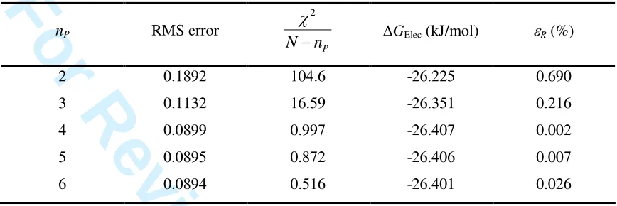
We have fitted the data of Figure 1 to polynomials of increasing degree,

following equation (7), and the results are shown in Table 1 (the respective fits are depicted in supporting information, Figure S1). It is clear that the root mean square

(RMS) error of the fit decreases significantly from a quadratic to a quartic polynomial, but then shows no significant change as nP is further increased. A statistical estimate of

the quality of the fit is given by the χ2 value, which should be of the same order as the

number of degrees of freedom of the fit29 (in this case, N-nP). The improvement is

remarkable upon increasing nP from 2 to 4, but there is only a small change by further

increasing the polynomial degree. Finally, the error in the value of the integral computed analytically from the fitting function relative to the value calculated by

numerical integration of the data using Simpson’s rule, denoted as εR, actually shows a

minimum at nP = 4. This analysis leads us to conclude that the electrostatic contribution

curve is ideally fitted by a polynomial of degree 4.

For Review. Confidential - ACS

Table 1 polynomial functions of increasing degree (– Results obtained by fitting the electrostatic contribution data for methanol to nP). nP RMS error

2 P

N n

χ

− ∆GElec (kJ/mol) εR (%)

2 0.1892 104.6 -26.225 0.690

3 0.1132 16.59 -26.351 0.216

4 0.0899 0.997 -26.407 0.002

5 0.0895 0.872 -26.406 0.007

6 0.0894 0.516 -26.401 0.026

Now that we have established the optimal fitting function, it is time to compare the precision of the numerical methods with the analytic integration as the

number of data points (N) is reduced. For this purpose, we have generated reduced data

sets with fewer λ values by removing points from the full data set, such that the points

in the reduced data sets were spaced as evenly as possible. Most of these reduced sets

(i.e., with N = 65, 33, 17, 9, 5, and 3) were generated by dividing the original number of intervals (128) by successive powers of 2, and so the points were all evenly distributed. For the other reduced sets (i.e., N = 24, 13, 11, and 7), only one or two points at the

extremities of the integration range were not evenly distributed. For each of the reduced data sets, the free energy was computed both numerically, using either the trapezoidal

rule, equation (4), or Simpson’s rule, equation (6), and analytically, after fitting the data set to a quartic polynomial. The fits using some of the reduced data sets, as well as for the full set, are shown as lines in Figure 1. In Figure 2, we plot the absolute error in the

free energy, relative to the reference case (numerical integration with Simpson’s rule using the complete 129-point data set), as a function of the number of points in the data

set, for the three integration methods considered. The full results of our analysis of the

[image:18.595.79.513.135.280.2]

For Review. Confidential - ACS

electrostatic component, including values of the fitting parameters, χ2 values for the fits, and total free energies, are given in Supporting Information, Table S8.

Figure 2: Absolute error in the electrostatic contribution to the free energy, relative to the result

for the full data set, as a function of the number of points used in the integration. Open circles

are for the trapezoidal rule, open diamonds for Simpson’s rule and full triangles for the

analytical integration of the fitting function.

Analyzing Figure 1, we can see that with as few as 5 evenly spaced data

points, the behavior of the entire curve is well captured by the fitting function. When N

is reduced even further, one runs into over-fitting problems, i.e., the polynomial degree

is higher than the number of data points available for the regression. In this situation, the number of degrees of freedom of the fit exceeds the information content of the data, and there is arbitrariness in the final fitting model. Indeed, for the data set with 3 points,

we have used a quadratic function, rather than a quartic – as can be seen from Figure 1 the results are not very satisfactory.

From Figure 2, we can see that using up to 17 points all three methods yield free energies that are within 0.05 kJ/mol from the reference value. However, if the

For Review. Confidential - ACS

number of points is reduced further, the error of the trapezoidal rule increases significantly. Remarkably, both the Simpson rule and the analytic integral based on the

fitting function perform extremely well down to 5 data points. This is understandable if we consider the shape of the curve (Figure 1) – the convex shape and monotonic

behavior means that the linear interpolation between successive points that is at the core of the trapezoidal rule will produce a systematic underestimation of the free energy. Naturally, this systematic error can be reduced by increasing the number of points. On

the contrary, both the piecewise quadratic interpolation of Simpson’s rule and the quartic polynomial fit are able to correctly capture the curvature of the data, and require

only a very small number of intermediate points to yield a precise free energy value. This finding is quite important if we take into account that the large majority of calculations of the electrostatic contribution to the free energy are carried out with fewer

than 17 points and using the trapezoidal rule to compute the integral. Thus it is likely that most results in the literature present a systematic bias that may be quite significant.

4.2 – Lennard-Jones component

We turn now to an analysis of the integration of the LJ contribution to the

free energy. The full data set, including the corresponding standard deviations, is provided in Table S5 and plotted in Figure 3 for both methane and methanol. The curve

for the LJ contribution is dominated by a prominent peak located between 0.2 and 0.3

for both solutes; it first increases smoothly at low values of λ, and decreases again

smoothly after the peak. This shape is much more complex than for the electrostatic contribution (Figure 1). It is also important to notice that the sampling errors are also

much larger than for the electrostatic contribution, particularly in the vicinity of the peak. This is shown more clearly in Figure S2 of the Supporting Information. The

For Review. Confidential - ACS

behavior of the LJ curve reflects two competing factors: unfavorable excluded volume effects due to cavity creation in the solvent and favorable solute-solvent interactions35.

This interpretation has formed the basis for our development of the fitting function, equation (18). In fact, it is important to notice that the data to the left of the peak are

very well fitted by our partial expression for the cavity formation term, equation (10), while the data to the right of the peak are well described by the expression derived for the attractive term, equation (16). These partial fits to the data, depicted in Figure 4 for

the case of methane, validate our approach in developing the fitting function for the LJ contribution to the free energy.

For Review. Confidential - ACS

Figure 3: Lennard-Jones contribution to the Hamiltonian derivative with respect to λ _{for: a)}

methane; b) methanol (open circles with error bars). The lines are fits to the full and reduced

data sets, as indicated, using equation (18).

For Review. Confidential - ACS

Figure 4: Partial fits to the LJ contribution for methane. The data at low λ were fitted to

equation (10), while the data for high λ were fitted to equation (16).

The full data sets were fitted to equation (18) and the results are shown as thick lines in Figure 3. As we can see, the function is able to correctly describe the data

in the entire region of interest, despite the large amount of statistical noise in the vicinity of the peak. Using the same procedure as in the case of the electrostatic

component, we have generated reduced data sets and carried out the integration using the two numerical methods and the fitting function. The fitted curves are shown as lines in Figure 3, while the full results of the analysis, including values of the fitting

parameters, χ2 values for the fits, and total free energies, are provided in Supporting Information, Tables S9 and S10. In Figure 5, we show the absolute error in the free energy, relative to the reference case, as a function of the number of points in the data

set, for the three integration methods considered.

For Review. Confidential - ACS

Figure 5: Absolute error in the LJ contribution to the free energy, relative to the result for the

full data set, as a function of the number of points used in the integration, for: a) methane; b)

methanol. Open circles are for the trapezoidal rule, open diamonds for Simpson’s rule and full

triangles for the analytical integration of the fitting function.

For Review. Confidential - ACS

It is clear from Figure 3 that the fitting function is able to correctly describe the trend of the Hamiltonian derivative even using only a small number of points in the

fit (a good description is obtained with as few as 11 points). With 9 points, the fitted curve starts to deviate significantly from the full data set, particularly in the case of

methane (see thick dashed line in Figure 3a), and with 7 points the performance is quite poor. The performance of the different integration methods can be assessed quantitatively by analyzing Figure 5. First of all, it is worth noticing that in general the

errors are larger and show more scatter than for the electrostatic component, which is caused by the higher degree of statistical noise in the simulated data. Furthermore,

Simpson’s rule now does not significantly outperform the trapezoidal rule – since the function has a maximum, the systematic error of the trapezoidal rule tends to cancel out after the full integration. As expected, the error tends to increase as the number of points

is reduced, but this decrease is not very pronounced down to N = 17. In this region, all three integration methods show a similar performance. As the number of points is

reduced further, the error of both numerical integration schemes increases significantly. Using the fitting function, however, one is able to maintain a good precision down to about 11 points, and the difference relative to the numerical methods is even more

marked for 9 points. Probably the most important conclusion of our analysis is that when considering a small number of intermediate stages (we recommend using 11 for

the LJ contribution) the fitting function always produces more precise results than the two numerical integration techniques.

At this point, it is worth commenting on the possibility of using different

fitting functions for the LJ component. Shyu and Ytreberg13 have performed a systematic analysis of polynomial fits to free energy data, but have only applied their

procedure to simple test cases with monotonous curves and analytical solutions. In more

For Review. Confidential - ACS

realistic situations, such as those presented here, polynomial functions are unable to correctly capture the behavior of the Hamiltonian derivative. In fact, even a fit to a

polynomial of degree 10 using the full data set shows unphysical oscillations near the integration limits (see Figure S3). We have also tested some alternative functional forms

(e.g., rational functions), but, although reasonable, their overall performance was not as good as that of equation (18). These studies are presented in detail in Section S.2 of the Supporting Information.

4.3 – Applicability test

Our study of different integration methods, performed above, focused on two

small solutes, so as to enable simulations at a large number of intermediate values of λ.

In this section, we assess whether the conclusions drawn from the analysis of the

prototype systems are applicable in realistic free energy calculations involving more

complex molecules. For that purpose, we attempt to compute the hydration energy of

2-methylbutanol and the hydration energy of a multifunctional compound (4-nitrophenol)

using the methodology proposed above.

Previously, we have seen that the deviation in the electrostatic contribution to the free energy was very small and practically independent of the integration method

down to N=17 (Figure 2). The same can be said of the LJ component down to N=33 (Figure 5). For that reason, we have carried out simulations for 2-methylbutanol and

4-nitrphenol using 17 points for the electrostatic component and 31 points for the LJ component, to serve as reference values. Our previous analysis showed that sufficiently precise free energies could be obtained with N=5 for the electrostatic component (using

the fitting function or Simpson’s rule) and N=11 for the LJ component (using the fitting function). Thus, we have generated reduced data sets with these values of N for each

For Review. Confidential - ACS

respective component. The full results of the fitting procedure are given in Supporting Information, Tables S11 to S14 (including additional reduced data sets that were tested).

Figure 6: Fits to the data for methylbutanol using the full and reduced data sets for: a)

electrostatic contribution using equation (7); b) Lennard-Jones contribution using equation (18).

For Review. Confidential - ACS

In Figure 6 we show the fits to the full and reduced data sets of 2-methylbutanol using equations (7) and (18) for the electrostatic and LJ contributions,

respectively. In both cases, the fits using the reduced data sets are able to provide a good description of the behavior of the Hamiltonian derivative. In Tables 2 and 3 we present

the reference values for each contribution (full data set integrated using the Simpson rule) as well as the deviations from this value using the reduced sets and different integration methods. The analysis of both solutes confirms our previous conclusions

based on methane and methanol – good results for the electrostatic component (error below 0.15 kJ/mol) are obtained using either the Simpson rule or the fitting function,

while for the LJ component, only the fitting function is able to provide sufficiently precise free energies (error of 0.15 kJ/mol) based on the reduced data sets. The results are even more striking for 4-nitrophenol, with errors below 0.05 kJ/mol obtained using

our suggested protocol, particularly considering the complexity of this multifunctional

molecule. This confirms our claim that a correct choice of integration method can

substantially improve the precision of solvation free energy calculations, even for complex solutes. Another way of thinking about this is to say that using our proposed integration methods one can make free energy calculations faster by a factor between 3

and 4, by reducing the necessary number of intermediate points, without significant loss in precision.

Table 2 – Results (in kJ/mol) for the two contributions to the hydration energy of

2-methylbutanol, and deviations from the reference value using different integration methods.

Electrostatic Lennard-Jones

∆GReference -26.86 9.62

Trapezoidal Reference

G G

∆ − ∆ 0.568 0.623

Simpson Reference

G G

∆ − ∆ 0.103 0.901

Analytic Reference

G G

∆ − ∆ 0.140 0.152

[image:29.595.166.435.625.724.2]

For Review. Confidential - ACS

Table 3 – Results (in kJ/mol) for the two contributions to the hydration energy of 4-nitrophenol,

and deviations from the reference value using different integration methods.

Electrostatic Lennard-Jones

∆GReference -33.39 1.75

Trapezoidal Reference

G G

∆ − ∆ 0.521 0.365

Simpson Reference

G G

∆ − ∆ 0.042 0.509

Analytic Reference

G G

∆ − ∆ 0.010 0.044

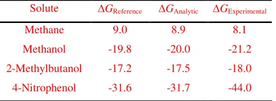
Table 4 summarizes our results for the total hydration energy of the four solutes considered. The reference values (from the full data sets) are compared to results

obtained using reduced data sets of the recommended size (11 for LJ and 5 for electrostatic) integrated using the fitting functions. Although it is not our aim here to

discuss the accuracy of the molecular model employed, it is nevertheless instructive to

compare our results with experimental data. Encouragingly, our results are close to

experimental values for the two simple solutes, and agree very well with experiment for

2-methylbutanol. For the case of 4-nitrophenol the agreement is worse, which illustrates

the weakness of current force-fields in predicting hydration free energies of

multifunctional compounds, as discussed elsewhere37.

Table 4 – Results for the total hydration energy (in kJ/mol) of the three solutes compared to

experimental data38, 39.

Solute ∆GReference ∆GAnalytic ∆GExperimental

Methane 9.0 8.9 8.1

Methanol -19.8 -20.0 -21.2

2-Methylbutanol -17.2 -17.5 -18.0

4-Nitrophenol -31.6 -31.7 -44.0

For Review. Confidential - ACS

5. Conclusions

In this work, we have carried out a detailed analysis of the effect of the

integration method on the calculation of solvation free energies using thermodynamic integration of molecular simulation data. By performing a very large number of

simulations (129 for each component) at intermediate values of the coupling parameter,

we have shown that the Hamiltonian derivative with respect to λ for the electrostatic

component displayed a smooth and monotonous behavior, while that for the

Lennard-Jones component had a more complex shape with a prominent peak at low λ values. For

the electrostatic component, the commonly used trapezoidal rule introduces systematic errors in the free energy as the number of intermediate points decreases. However, using either Simpson’s rule or a fitting polynomial of degree 4, these errors are significantly

reduced and one is able to obtain precise free energies with as few as 5 intermediate points. For the LJ component, however, both numerical integration methods show

approximately similar performances, with the errors increasing substantially as the number of points decreases below about 17. We have derived a physically-based fitting function that is able to provide a good description of the LJ Hamiltonian derivative

throughout the entire integration interval. Analytical integration of this fitting function produces accurate free energies with as few as 11 intermediate points. It is important to

notice, however, that convergence of the individual simulations is a requirement for obtaining precise free energies. Indeed, if the data set is not sufficiently converged, no integration method (including regression) will produce precise estimates. Our data were

obtained using sampling times of 5 ns for each intermediate point, and convergence was checked thoroughly.

Based on our study of hydration of simple solutes, we are able to recommend the following protocol for free energy calculations using thermodynamic integration: i)

For Review. Confidential - ACS

for the electrostatic component, one should run simulations at 5 evenly spaced values of λ and integrate the data using either Simpson’s rule or by fitting to a quartic

polynomial; ii) for the LJ component, one should run 11 simulations at evenly spaced

points, fit the data to equation (18), and calculate the free energy from the analytic integral of the fitting function, equation (20).

We have subsequently tested this protocol for more demanding cases –

hydration of 2-methylbutanol and 4-nitrophenol. The results obtained confirm our previous conclusions, thus showing that the above protocol is robust and can be applied

for the solvation of more complex solutes.

In summary, the use of an appropriate integration method can significantly

improve the precision of free energy calculations using thermodynamic integration, for a given computational cost, or, alternatively, can make the calculations much faster for a given precision level. The integration error implicit in the TI method is commonly seen

as a disadvantage of this approach relative to other methods, like thermodynamic

perturbation theory. Our contribution significantly reduces this disadvantage, making TI

even more competitive. We believe such improvements are required so that solvation free energy data can begin to be routinely employed in force-field parameterization, and can play a more active part in drug design efforts. Although our proposed protocol and

choice of fitting functions is specific to solvation free energy calculations, the principles

of the method may be extended to other types of free energy calculation (e.g., potentials

of mean force), with appropriate adaptations in the functional forms and in the required

number of intermediate points.

For Review. Confidential - ACS

Acknowledgments

The authors are grateful for the support provided by Fundação para a Ciência e a

Tecnologia (FCT) Portugal, through projects FEDER/POCI/2010 and

REEQ/1164/EQU/2005. NMG also acknowledges his Ph.D. scholarship

SFRH/BD/47822/2007 from FCT.

Supporting Information Available

Detailed van der Waals parameters, point charges, bond stretching, bond angle bending

and torsional force constants as well as detailed bonded and nonbonded potential

parameters are provided for all compounds studied. The full data set for the different

contributions to the derivative of the Hamiltonian with respect to λ and the full results of the

analysis of the LJ and electrostatic terms are also provided. Finally, results obtained by using

alternative fitting functions to the one presented in the paper for the LJ component of the free

energy are illustrated. This information is available free of charge via the Internet at

http://pubs.acs.org/.

References

1. Gilson, M.; Zhou, H., Calculation of protein-ligand binding affinities. Annu. Rev.

Biophys. Biomol. Struct. 2007, 36, 21-42.

2. Jorgensen, W. L., The many roles of computation in drug discovery. Science 2004, 303

(5665), 1813-1818.

3. Mobley, D. L.; Bayly, C. I.; Cooper, M. D.; Shirts, M. R.; Dill, K. A., Small Molecule

Hydration Free Energies in Explicit Solvent: An Extensive Test of Fixed-Charge Atomistic

Simulations. J. Chem. Theory Comput. 2009, 5 (2), 350-358.

4. Guthrie, J. P., A Blind Challenge for Computational Solvation Free Energies:

Introduction and Overview. J. Phys. Chem. B 2009, 113 (14), 4501-4507.

5. Oostenbrink, C.; Villa, A.; Mark, A. E.; Van Gunsteren, W. F., A biomolecular force

field based on the free enthalpy of hydration and solvation: The GROMOS force-field

parameter sets 53A5 and 53A6. J. Comp. Chem. 2004, 25 (13), 1656-1676.

6. Kirkwood, J. G., Statistical Mechanics of Pure Fluids. J. Chem. Phys. 1935, 3, 300-313.

For Review. Confidential - ACS

7. C. Chipot; Pohorille, A., Free Energy Calculations - Theory and Applications in

Chemistry and Biology. Springer: Berlin, 2007.

8. Shirts, M. R.; Pitera, J. W.; Swope, W. C.; Pande, V. S., Extremely precise free energy

calculations of amino acid side chain analogs: Comparison of common molecular mechanics

force fields for proteins. J. Chem. Phys. 2003, 119 (11), 5740-5761.

9. Straatsma, T.; Berendsen, H., Free energy of ionic hydration: analysis of a

thermodynamic integration technique to evaluate free energy differences by molecular dynamics

simulations. J. Chem. Phys. 1988, 89, 5876-5886.

10. Smith, E. J.; Bryk, T.; Haymet, A. D. J., Free energy of solvation of simple ions:

molecular-dynamics study of solvation of Cl- and Na+ in the ice/water interface. J. Chem. Phys. 2005, 123, 034706.

11. Swope, W.; Andersen, H., A molecular dynamics method for calculating the solubility

of gases in liquids and the hydrophobic hydration of inert-gas atoms in aqueous solution. J.

Phys. Chem. 1984, 88, 6548-6556.

12. Hummer, G.; Pratt, L. R.; Garca, A. E., Free energy of ionic hydration. J. Phys. Chem.

1996, 100 (4), 1206-1215.

13. Shyu, C.; Ytreberg, F. M., Reducing the bias and uncertainty of free energy estimates by

using regression to fit thermodynamic data. J. Comput. Chem. 2009, 30, 2297-2304.

14. Hess, B.; Kutzner, C.; van der Spoel, D.; Lindahl, E., GROMACS 4: Algorithms for

highly efficient, load-balanced, and scalable molecular simulation. J. Chem. Theory Comput.

2008, 4, 435-447.

15. Jorgensen, W. L.; Maxwell, D. S.; Tirado-Rives, J., Development and testing of the

OPLS all-atom force field on conformational energetics and properties of organic liquids. J. Am.

Chem. Soc. 1996, 118 (45), 11225-11236.

16. Berendsen, H. J. C.; Grigera, J. R.; Straatsma, T. P., The missing term in effective pair

potentials. J. Phys. Chem. 1987, 91 (24), 6269-6271.

17. Hess, B.; Bekker, H.; Berendsen, H. J. C.; Fraaije, J., LINCS: A Linear Constraint

Solver for Molecular Simulations. J. Comp. Chem. 1997, 18 (12), 1463-1472.

18. Miyamoto, S.; Kollman, P. A., SETTLE - An Analytical Version of the SHAKE and

RATTLE agorithm for Rigid Water Molecules. J. Comp. Chem. 1992, 13 (8), 952-962.

19. Garrido, N. M.; Jorge, M.; Queimada, A. J.; Economou, I. G.; Macedo, E. A., Molecular

Simulation of the Hydration Free Energy of Barbiturates. Fluid Phase Equilib 2009,

doi:10.1016/j.fluid.2009.11.022.

20. Lee, F. S.; Warshel, A., A local reaction field method for fast evaluation of long-range

electrostatic interactions in molecular simulations. J. Chem. Phys. 1992, 97 (5), 3100-3107.

21. van Gunsteren, W.; Berendsen, H., A leap-frog algorithm for stochastic dynamics. Mol.

For Review. Confidential - ACS

22. Van Gunsteren, W. F.; Berendsen, H. J. C., Algorithms for Brownian Dynamics. Mol.

Phys. 1982, 45 (3), 637-647.

23. Berendsen, H. J. C.; Postma, J. P. M.; Vangunsteren, W. F.; Dinola, A.; Haak, J. R.,

Molecular Dynamics with Coupling to an External Bath. J. Chem. Phys. 1984, 81 (8),

3684-3690.

24. Beuler, T. M., R; van Schaik, RC; Gerber, PR; van Gunsteren, WF, Avoiding

singularities and numerical instabilities in free energy calculations based on molecular

simulations. Chem. Phys. Lett. 1994, 222, 529-539.

25. Pitera, J. W.; Van Gunsteren, W. F., A comparison of non-bonded scaling approaches

for free energy calculations. Mol. Sim. 2002, 28 (1-2), 45-65.

26. Mobley, D. L.; Dumont, E.; Chodera, J. D.; Dill, K. A., Comparison of charge models

for fixed-charge force fields: Small-molecule hydration free energies in explicit solvent. J. Phys.

Chem. B 2007, 111 (9), 2242-2254.

27. Liu, D. C.; Nocedal, J., On the Limited Memory BFGS Method for Large Scale

Optimization. Math. Program. 1989, 45 (3), 503-528.

28. Flyvbjerg, H.; Petersen, H., Error estimates on averages of correlated data. J. Chem.

Phys. 1989, 91 (1), 461-466.

29. Press, W.; Teukolsky, S.; Vetterling, W.; Flannery, B., Numerical recipes in C. 2 ed.;

Cambridge University Press: Cambridge, 1992.

30. Pierotti, R. A., A scaled particle theory of aqueous and nonaqueous solution. Chem.

Rev. 1976, 76 (6), 717-726.

31. Stillinger, F. H., Structure in aqueous solutions of nonpolar solutes from the standpoint

of scaled-particle theory. J. Sol. Chem. 1973, 2 (2/3), 141-158.

32. Reiss, H.; Frisch, H. L., Statistical mechanics of rigid spheres. J. Chem. Phys. 1959, 31

(2), 369-380.

33. Westergren, J.; Lindfors, L.; Hoglund, T.; Luder, K.; Nordholm, S.; Kjellander, R., In

silico prediction of drug solubility: 1. Free energy of hydration. J. Phys. Chem. B 2007, 111 (7),

1872-1882.

34. Grace Software is available free of charge at: http://plasma-gate.weizmann.ac.il/Grace/

acessed: October 22, 2009.

35. Wan, S. Z.; Stote, R. H.; Karplus, M., Calculation of the aqueous solvation energy and

entropy, as well as free energy, of simple polar solutes. J. Chem. Phys. 2004, 121 (19),

9539-9548.

36. Shirts, M. R.; Pande, V. S., Solvation free energies of amino acid side chain analogs for

common molecular mechanics water models. J. Chem. Phys. 2005, 122 (13), 134508.

For Review. Confidential - ACS

37. Garrido, N. M.; Queimada, A. J.; Jorge, M.; Economou, I. G.; Macedo, E. A., Molecular

Simulation of Absolute Hydration Gibbs Energies of Polar Compounds. Submitted for

Publication 2010.

38. Michielan, L.; Bacilieri, M.; Kaseda, C.; Moro, S., Prediction of the Aqueous Solvation

Free Energy of Organic Compounds by Using Autocorrelation of Molecular Electrostatic

Potential Surface Properties Combined with Response Surface Analysis. Bioorg. Med. Chem.

2008, 16 (10), 5733-5742.

39. Cabani, S.; Gianni, P.; Mollica, V.; Lepori, L., Group Contributions to the

Thermodynamic Properties of Non-Ionic Organic Solutes in Dilute Aqueous Solution. J. Sol.

Chem. 1981, 10 (8), 563-595.