http://pio.sagepub.com/
Reliability
Engineers, Part O: Journal of Risk and
http://pio.sagepub.com/content/224/4/322
The online version of this article can be found at:
DOI: 10.1243/1748006XJRR304
2010 224: 322
Proceedings of the Institution of Mechanical Engineers, Part O: Journal of Risk and Reliability
T Bedford and L Walls
Evaluation of elicitation methods to quantify Bayes linear models
Published by:
http://www.sagepublications.com
On behalf of:
Institution of Mechanical Engineers
be found at:
can Proceedings of the Institution of Mechanical Engineers, Part O: Journal of Risk and Reliability Additional services and information for
http://pio.sagepub.com/cgi/alerts
Email Alerts:
http://pio.sagepub.com/subscriptions
Subscriptions:
http://www.sagepub.com/journalsReprints.nav
Reprints:
http://www.sagepub.com/journalsPermissions.nav
Permissions:
http://pio.sagepub.com/content/224/4/322.refs.html
Citations:
What is This?
- Dec 1, 2010
Version of Record
Evaluation of elicitation methods to quantify
Bayes linear models
g
M Revie∗, T Bedford,andL Walls
Department of Management Science, University of Strathclyde, Strathclyde, UK
The manuscript was received on 30 November 2009 and was accepted after revision for publication on 25 May 2010.
DOI: 10.1243/1748006XJRR304
Abstract: The Bayes linear methodology allows decision makers to express their subjective beliefs and adjust these beliefs as observations are made. It is similar in spirit to probabilistic Bayesian approaches, but differs as it uses expectation as its primitive. While substantial work has been carried out in Bayes linear analysis, both in terms of theory development and appli-cation, there is little published material on the elicitation of structured expert judgement to quantify models. This paper investigates different methods that could be used by analysts when creating an elicitation process. The theoretical underpinnings of the elicitation methods devel-oped are explored and an evaluation of their use is presented. This work was motivated by, and is a precursor to, an industrial application of Bayes linear modelling of the reliability of defence systems. An illustrative example demonstrates how the methods can be used in practice.
Keywords: Bayes linear models, elicitation; expert judgement, reliability analysis, uncertainty analysis
1 INTRODUCTION
The Bayes linear theoretical framework is a quanti-tative methodology capable of expressing subjective beliefs and reviewing these beliefs once observations have been made [1]. The Bayes linear methodology offers decision makers a method to structure, study, and assess the relationships between coherent partial belief statements. Once observations are made, these beliefs are adjusted by linear fitting (as opposed to the traditional conditioning rules of Bayes theorem) using equations (1) and (2) whereX is a vector of quantities of interest andDis the observed data.
ED(X)=E(X)+cov(X,D)(var−1(D))(D−E(D)) (1)
varD(X)=var(X)−cov(X,D)(var−1(D))cov(D,X) (2)
It is natural to view the Bayes linear methodology as an inferential tool that is similar in philosophy to
*Corresponding author: Department of Management Science, University of Strathclyde, Graham Hills, Building 40, George Street, Strathclyde G1 1QE, UK.
email: [email protected]
‘traditional’ Bayesian approaches. However, it has a number of distinct features that give it certain advantages, such as simplicity and tractability, over these ‘traditional’ approaches when modelling prob-lems [2]. As such, more complex problems could be modelled given the same amount of time and effort. While it is beyond the scope of this paper, it is assumed that those wishing to adopt this modelling are sympa-thetic to the subjective Bayesian paradigm. Further reading and debate on the objective versus subjec-tive Bayesian paradigm can be found in references [3] and [4], and other papers within that special issue.
The Bayes linear methodology has been applied in projects in many different areas. For example: Craig
et al. [5] use the Bayes linear methodology to esti-mate the level of hydrocarbons in a reservoir based on a computer simulation; Coolenet al. [6] to reduce the number of software tests required to remove faults from software; O’Haganet al. [7] to estimate the assets of sections of the UK water industry; Farrowet al. [8] to support decision making within a brewery; and Revie [9] to support reliability decision making for the UK Ministry of Defence (MOD).
how to build the model, how to elicit the neces-sary values, or how to carry out sensitivity analysis, all remain relatively underdeveloped. In particular, developing pragmatic elicitation approaches has been largely ignored. For example, reference [5] does not focus on elicitation but refers to it as an area of gen-eral interest. In reference [10], the general principles of elicitation for variance and covariance are dis-cussed, but the reader is not given guidance on how this may be carried out. More guidance is given in reference [8]. A comprehensive review of the Bayes linear theory and methods is given by Goldstein and Wooff [11], but they consider the issue of elicitation briefly. A non-exhaustive list of potential methods that could be used to populate a Bayes linear model, rang-ing from specifyrang-ing quantiles to usrang-ing historical data from samples in related populations, is presented in reference [11].
Naturally, Goldstein and Wooff [11] do not wish to give strict guidelines that may not be applicable in all cases; however, there is no clear guidance on how to specify the quantiles and elicit the expecta-tion, variance, and covariances. Only reference [7] devotes substantial effort to discussing how elicitation is carried out. In this case, the expert stated a mean for the expectation while the variance was calculated from an elicited standard deviation. The authors are open in their concerns about this elicitation method as they state ‘this expression of standard deviation, as well as the sweeping interpretation of a point esti-mate as a mean, is not designed to produce the most careful and accurate of prior judgements’ [7]. This method may be effective in cases where the output is robust to changes in the prior beliefs, but in other cases a more structured elicitation procedure may be desirable.
To support decision makers in applying Bayes linear models more widely, clear procedures are required. Indeed, the research reported in the current paper is motivated by the authors’ involvement in reliability modelling during defence procurement projects [9], which required the development of methods to sup-port implementation of Bayes linear models that could be used with UK MOD decision makers. Prior to practical implementation within the live projects, a study was conducted of methods that could be used to support elicitation and specification of the model. This paper reports the development and evaluation of the methods proposed to overcome one of the main challenges of building a Bayes linear model. Alter-native methods for quantifying a Bayes linear model through elicitation of the expectation and covari-ance structure are investigated and the results used to inform the recommendations. Section 2 gives an introduction to elicitation and the different meth-ods that could be used. Section 3 presents a com-parative study to evaluate methods and makes a
recommendation on which method should be used. Section 4 presents an illustrative example based on an industrial application. Section 5 discusses future research.
2 METHODS FOR POPULATING A BAYES LINEAR MODEL
Elicitation is a key part of the process in populating a Bayes linear model. The purpose of an elicitation session is to gather quantitative data that represent the belief of the person being elicited [12]. This is important in many problems where empirical data may not exist to quantify the uncertainty of different probabilities. The history of the application of expert judgement is examined by Cooke [13] and a frame-work for the defensible elicitation and use of expert judgement, methods for the assessment of the qual-ity and usefulness of stated values, and methods to combine judgements are proposed.
Effort has been spent in documenting how elicita-tion has been carried out [14–18]. A number of books have been written discussing elicitation, notably ref-erences [13] and [19–23]. These books present a comprehensive treatment of the processes involved in eliciting expert judgement. They describe the pro-cesses of planning and conducting the elicitation, identifying appropriate experts, designing question-naires, recording judgements and managing biases, and finally analysing and aggregating experts’ judge-ments. These books also provide a comprehensive summary of the biases that may arise during an elici-tation session such as availability, representativeness, and anchoring [24], the high-level steps required dur-ing an elicitation process, and the different methods available to elicit probability distributions.
to attempt to minimize these biases and to ensure that the beliefs stated are coherent.
There is consensus in the literature regarding which high-level steps should be carried out during an elici-tation process [23]. It is suggested that any elicitation process should include seven stages: background, identification, and recruitment of expert, motivating experts, structuring and decomposition, probabil-ity and assessment training, probabilprobabil-ity elicitation and verification, and aggregation of expert’s prob-ability distributions [30]. Much of the work carried out in developing elicitation processes has focused on developing methods for multiple experts [17,30,31]. However, on other projects, such as reference [9], only one expert was used during the modelling. As such, high-level steps for projects with only one expert are also required.
Processes which focus on only one expert have been proposed [12,32]. A four-stage process suit-able for scenarios where elicitation is carried out with single experts or decision makers is discussed in reference [12]. This four-stage process is set-up, elicitation of summaries, fit distribution, and assessing adequacy of elicitation. This process was developed for probabilistic models. In order to apply this within the Bayes linear framework, one impor-tant change is required. Instead of ‘fit distribu-tions’, within the developed process, this will be changed to ‘calculate mean and covariances’. Alter-native processes may elicit expectations and variances directly.
2.1 Eliciting means and variances
Elicitation techniques should be designed to fit the way people think instead of forcing experts to answer questions in a specific format [21]. An expert in a subject domain should not be viewed as an expert in statistics or probability theory; any elicitation method must be as simple as possible for experts to communicate their beliefs accurately. Within a Bayes linear framework, the decision maker’s belief about the expectation, variance, and covariance between the parameters in the model must be assessed.
Eliciting means and covariances directly is difficult as experts do not naturally think in these terms – ‘experts should not be asked to estimate moments of a distributions (except possibly the first moment); they should be asked to assess quantiles or proba-bilities’ [14]. Others [33] agree that it is necessary to use quantiles to estimate at least the variance of an expert’s subjective belief. From these quantiles, the mean and variance can be calculated. Methods have been developed which focus on eliciting differ-ent percdiffer-entiles of a variable and then calculating the mean and variance of the variable directly. A summary
is provided in reference [12] of the different elic-itation methods. All of these methods, however, focus on fitting a distribution to the elicited quan-tiles. As the Bayes linear method does not assume any distributional form on the prior beliefs, the present authors would prefer an elicitation method which does not rely on a distributional form being assumed.
As touched upon earlier, only reference [7] has discussed in detail the different methods to elicit the necessary values. This paper was extended by O’Hagan [15] to describe additional methods to elicit variance. For the expectation, no special elicitation procedure was developed. Instead, only potential pitfalls were identified for senior personnel to pass on to engineers. For the variance, O’Hagan [15] assumed either a normal or log-normal distribution and elicited three percentiles: the median, MX; the 17th percentile, LX; and the 83rd percentile, UX. If UX −MX is substantially greater than MX −LX, then a log-normal distribution is assumed. No guid-ance is given in reference [15] on the numerical value such thatUX −MX is substantially greater than
MX −LX.
No justification is given in reference [15] as to why the 17th and 83rd percentiles are used, other than that the author felt that experts were overconserva-tive when specifying the interval between the 25th and 75th percentiles. It is acknowledged by O’Hagan [15] that this is in contrast to other authors, such as Alpert and Raiffa [34] and Murphy and Winkler [35], who found that people were well calibrated at these inter-vals. Larger intervals, such as a 99 per cent range, were strongly influenced by events of small prob-abilities [15], and as such, people were not well calibrated at this level. This is supported by evi-dence [29,34,36]. While reference [15] states that this method is ‘very crude and simplistic’, owing to the number of quantities required to populate the model, a simple approach was adopted. This method appears reasonable if the expert’s beliefs are regu-larly normal or log-normal. In situations where this assumption cannot be made, an alternative method is required.
a mean,µX and variance,σX2 forX. The Pearson and Tukey formulae are as follows
µX =0.63X0.5+0.185(X0.05+X0.95) (3)
σ2 X =
⎡
⎣ X0.95−X0.05 3.29−0.1
σ0
⎤ ⎦
2
(4)
where
=X0.95+X0.05−2X0.5
and
σ0=
X0.95+X0.05 3.25
2
The three-point Pearson and Tukey method per-formed almost identically to the five-point Pearson and Tukey method when assessing the variance [38].
A number of alternative methods have been pro-posed in the literature; the PERT (Program Evaluation Research Task) method [39], Moder–Rodgers [40], Davidson–Cooper [41], and Swanson–Megill [42]. Comparisons with these methods using the beta dis-tribution found that the three-point Pearson and Tukey method performed best when assessing the mean and was second only to the five-point Pearson and Tukey method. The maximum error across a set of beta distributions using the Pearson and Tukey method was found to be−1.7 per cent [43]. This was substantially lower than the maximum error found with the Moder–Rodgers method, −20.7 per cent, Davidson–Cooper method, −17.7 per cent, and the PERT method, 5506 per cent. This analysis was extended by Johnson [44] to measure the accuracy of the Pearson and Tukey method to alternative distribu-tions such as the gamma and log-normal. Johnson [44] found that the Pearson and Tukey method was robust when assessing the mean with a maximum error of 0.05 per cent for the gamma and 0.68 per cent for the log-normal. For the standard deviation, the method was again robust for the gamma distribution with a maximum error of 0.7 per cent; however, for the log-normal distribution, the maximum error for the standard deviation was 11.6 per cent. Since the current analysis is being carried out within a relia-bility context, the present authors are interested in assessing how the Pearson and Tukey method copes with right-skewed lifetime distributions such as those discussed.
As the method is robust across a range of possible distributions, the authors believe that the three-point Pearson and Tukey method is adequate for eliciting the mean and variance in most situations.
2.2 Eliciting covariances
In almost all complex real-world decision-making problems it is inevitable that there exists a degree of dependency between the variables being modelled. Where there is a lack of data on the relationships between variables, subjective expert judgement is crucial in modelling these problems and in provid-ing information on the strength of the dependencies between variables [21]. While attention has been given to building influence diagrams and modelling the qualitative dependencies between different variables, less attention has been given to how to assess or elicit the quantitative dependency from experts [45]. This is a crucial part of the modelling as the output of any model could be sensitive to the dependency values specified.
Elicitation methods must have strong theoretically rigorous foundations, be capable of generalization to a wide range of different problems, and should have a clear intuitive interpretation [45]. In addition to this, those using the techniques should find them ‘easy and credible’ [45]. In the Bayes linear framework, covariance is the measure of dependency; however, eliciting the covariance directly from an expert is likely to encounter problems [12]. Instead, a method to cal-culate the covariance from other elicited values must be used.
Owing to the way in which prior beliefs are speci-fied in a Bayes linear framework, there are a limited number of ways in which the dependency value between two variables, i.e. cov(X,Y), can be specified. Four different methods of determining the depen-dency between two variables, X and Y, in a Bayes linear framework have been identified: direct cal-culation (DC); direct elicitation of correlation (C); adjusted expectation (AE); and adjusted uncertainty (AU). Details of each method are given below. In each example described below, the analyst is attempting to elicit the beliefs from an expert who is referred to as ‘she’. For each method, two variables are modelled using the formulaY =αX+R, where it is assumed that
X andRare uncorrelated. In this case,X is viewed as an explanatory variable ofY.
2.2.1 Direct calculation (DC)
It is assumed that the expert has already specified her E(X) and var(X) using the Pearson and Tukey equations (3) and (4). The expert then specifiesE(Yt), her new belief ofE(Y)given thatE(X)has increased byt. From this,αcan be calculated using the formula [E(Yt)−E(Y)]/t. She then specifies her 5, 50, and 95 percentiles for the uncertain variableR. This can be achieved by asking her, ‘Given thatX is known to be
˜
E(Y) = αE(X)+E(R), var(Y) = α2var(X)+var(R), and cov(X,Y)=αvar(X).
During the elicitation, the analyst must specify x˜. A value for x˜ is chosen such that the expert is com-fortable specifying quantiles forY, given that she has observedy˜. If she does not feel comfortable specify-ing for this x˜, the analyst should explore alternative values.
2.2.2 Direct elicitation of correlation (C)
For C, the expert first has to specifyE(X),E(Y), var(X), and var(Y). The expert is then asked to state her assessment of the correlation between variables X
and Y. To do this, she must have an understand-ing of correlation. From corr(X,Y), cov(X,Y)may be calculated using cov(X,Y)=corr(X,Y)σXσY.
2.2.3 Adjusted expectation (AE)
For AE, again the expert must specify E(X), E(Y), var(X), and var(Y). She is then told that she is to con-sider her belief about X given that she can observe the true value for variableY. Supposing that the true value of variableYisy˜, she is then asked to specify her new belief aboutE(X),EY(X)=XY, given that she has observedy˜. By rearranging the formula for adjusted expectation (1), cov(X,Y)can be calculated using
cov(X,Y)=
EY(X)−E(X)
Y−E(Y)
var(Y)
= XY −X ˜
y−Y
σ2
Y (5)
From cov(X,Y), it is possible to calculateα. AsY =
αX+R, thus cov(X,Y)=αvar(X)so that
α= cov(X,Y)
var(X)
In order to ensure that the expert is coherent, there are limitations on the values that can be specified. As var(Y)and var(X)have already been specified, there exists an upper and lower bound on the value forα. Since var(R)0 andα2var(X)var(Y), this implies that
α
var(Y)
var(X)
Inserting
α
var(Y)
var(X)
and assuming thaty˜ Y into equation (1) gives
XY X +
var(X)
var(Y)(y˜−Y) (6)
If the expert specifies a belief greater than the value given by equation (6), then
cov(X,Y) > α
var(Y)
var(X)
However, as this is an upper bound, one of the other values has been incoherently specified. In this case, the analyst must revisit and reassess with the expert the previously elicited values.
As with the DC method, the analyst must specifyy˜. A value for y˜ is chosen such that the expert is com-fortable specifyingXY, given that she has observedy˜. As with the DC method, if she does not feel comfort-able specifying for thisy˜, the analyst should explore alternative values.
2.2.4 Adjusted uncertainty (AU)
For AU, again the expert must specify E(X), E(Y), var(X), and var(Y). She is then told that the value that she initially believed variableY would take, i.e.
Y, has been observed. She is then asked to specify her adjusted variance forX,σ2
X|Y given that she now knows the true value ofY. To calculate the variance, equation (4) can be used. Rearranging equation (2), cov(X,Y)can be calculated using the formula
cov(X,Y)=(var(X)−varY(X))var(Y)) (7) As with AE, there are limitations on the values that the expert can specify in order to maintain coherency. In this case, the expert cannot specify that the adjusted variance, varY(X)is greater than the prior variance, var(X). In addition, in order that varY(X) 0, cov(X,Y)√var(X)var(Y).
2.2.5 Setting hypothetical values
In DC and AE, the analyst must specify hypotheti-cal values. The expert then states their belief, given that they have hypothetically observed these new val-ues. The analyst should specify a value with which the expert is comfortable. This could clearly be multiple values. In order to assess the consistency of the expert, the analyst could choose multiple hypothetical values and ensure that the covariances across these multiple scenarios are similar.
3 EXPERIMENTAL STUDY TO EVALUATE ALTERNATIVE ELICITATION METHODS
given in section 2 is most appropriate to adopt during an elicitation session. In order to achieve this, three dependencies have been presented to participants and for each of the four methods above, a correla-tion value is calculated. These dependencies are: life expectancy between males and females in the same country; height and weight of male students at a uni-versity; and mean miles to failure (MMTF) between a population of vehicles and the miles to failure of a single observed vehicle. These dependencies have been chosen in order that three different scenarios are investigated. Scenario 1 assesses two dependencies with the same unit of measure; scenario 2 assesses two dependencies with different units of measures; and scenario 3 assesses the dependency between a population and a single observation. These scenar-ios represent the types of dependency that decision makers are likely to have to model during a risk and reliability analysis. For each of these three depen-dencies, expectations and variances for each of the variables have been gathered and four correlation val-ues have been elicited from each participant using each of the described methods.
A total of 23 participants, all of whom were post-graduate students of the University of Strathclyde, have taken part in the study. While none of the par-ticipants received formal training in the Bayes linear methodology, an example was used to explain how to interpret the values. These participants can be partitioned into three distinct groups; ten MSc stu-dents in operational research, nine PhD stustu-dents from the Department of Management Science, and four PhD students from the University of Strathclyde. The MSc students had all recently carried out a class in statistics, and all the PhD students had attended a short course in advanced quantitative methods. All had learned about correlation, means, and vari-ances. Within the MSc students and the PhD students there was a mix of statistical knowledge, as some had undergraduate degrees in either mathematics or statistics.
There has been criticism that much of the empiri-cal evidence gathered to assess elicitation techniques relies heavily on university students as the subject group (O’Haganet al. [23]). It is dangerous to assume that the findings from this group will necessarily trans-late across to other populations. While it is necessary to be wary about the deductions that can be made from these types of experimental study, it is also necessary to be pragmatic. For example, in the cur-rent case it was necessary to pre-test methods so that an appropriate one could be selected for imple-mentation within the industrial projects. The authors judged that the variation in the statistical knowledge of the selected students matched those of typical engi-neers with whom they would work in the reliability applications.
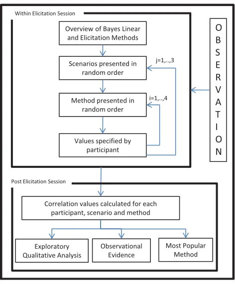
Fig. 1 Key stages of study
The students were split over three sessions. Each session lasted approximately 1 h. During this time, none of the students complained about the speci-fications being cognitively challenging or of fatigue. To try to minimize anchoring and potential learning, the three scenarios described above were presented in a random order. Within each scenario, the four methods for collecting the covariance were presented in a random order. Figure 1 summarizes the study design involving the process for conducting the elic-itation with the participants, as well as gathering observational data from them about methods and the follow-up analysis.
3.1 Criteria to evaluate methods
In order to extract as much information as possible about the performance of the alternative elicitation methods from the limited sample of participants, three elements of analysis were conducted: formal checks on coherency; feedback from participants; and observations of the elicitation process.
[image:7.595.315.551.76.361.2]then 95 per cent of all observed values of X are within that bound. However, Kadane and Wolfson [14] believe that calibration is not necessary, as elicita-tion is not used to elicit ‘perfect’ opinion but, instead, to elicit ‘expert’ opinion. It is hoped that identify-ing a ‘good’ expert will lead to the expert’s belief and reality coinciding. If a method captures the subjective belief of an expert, then the method is described as accurate. This poses a significant prob-lem, as traditional techniques cannot be used to determine if the elicited prior is a ‘good’ fit to the ‘true’ prior [29].
In addition to verification, coherence, and cal-ibration to measure the accuracy of an elicitation approach, another important consideration is practi-cality. It is necessary to be flexible and take account of the uniqueness of each project. For complicated mod-els or application-specific modmod-els, general elicitation methods are not desirable. Instead, the elicitation method chosen should be determined by ‘examin-ing the nature of the problem and whether or not the parameters have intrinsic meaning to the expert’ [14]. Therefore, it is unlikely that a single method for eliciting covariance will be recommended. Instead, scenarios where each covariance method might be most appropriate will be highlighted.
Recall the post-elicitation stage of the study demon-strated in Fig. 1. The first stage of analysis is to carry out exploratory quantitative analysis to determine if any of the methods produces values that are inconsistent with the participants’ beliefs. Since these elicitation techniques aim to gather the opinion of only the expert, any attempt to validate the techniques can be done only through other statements of belief by the same expert. In this example, it is not possible to determine which of the four techniques is capturing the ‘true’ belief of the respondent; however, it is pos-sible to discount some of the responses for each of the methods.
Second, the methods are evaluated qualitatively using observational evidence gathered during the elic-itation sessions and interviews carried out after the session with participants who volunteered to provide feedback. These interviews focused upon inconsisten-cies in the participants’ responses. Information has been gathered regarding why the participant speci-fied a given value and in which of the four methods they had most confidence.
The third stage of analysis is to determine which method is the most popular among the participants. For each dependency, each respondent has been asked to comment on which method they preferred. This is because it is unlikely that any method with which the participant is uncomfortable is likely to pro-duce accurate results. It is beneficial to gain an under-standing of how those unfamiliar with covariance techniques feel about them.
3.2 Analysis and results
For each of the three scenarios, all the participants agree that there is a relationship between the vari-ables, i.e. the correlation between the variables does not equal zero. All the participants also agree that the relationship is not perfect, i.e. the correlation is not equal to one. Finally, all the participants agree that the relationship is positive, i.e. the correlation is positive. For each of the elicitation methods, 23 participants specified covariance values for each of the three sce-narios. From this, 69 correlation values have been calculated for each of the four methods. Each cor-relation is categorized as one of three: acceptable, inconsistent, or incoherent. Acceptable is defined as being a correlation value of between 0 and 1. Incoher-ent is defined as producing a correlation value outside
−1 and 1. Any correlation value of 0, 1, or negative is defined as inconsistent. Table 1 summarizes the results.
From Table 1, it can be seen that the AU method is unlikely to be a useful method for gathering the covariance value from an expert. On three occasions, it produces correlation values that are beyond the acceptable range and on 25 occasions, it produces val-ues that are inconsistent – all of which were correlation values of 0. From the qualitative evidence gathered, some participants believed that learning about one variable would change their belief about the expecta-tion of the other variable, but not necessarily change their uncertainty about that belief.
[image:8.595.302.541.657.759.2]A previous study [28] observed that experts do not naturally think within a Bayesian theoretical frame-work. In the present study, it is apparent that many of the participants do not adjust their beliefs in a sim-ilar way to the Bayes linear method updating rule. While they all agree that a relationship exists, they do not all believe that their uncertainty would drop. This is in contrast to the Bayes linear methodology in which the adjusted variance is smaller than the orig-inal variance. In addition, out of the 69 responses, only seven participants believed that the AU method was the easiest method to use. Therefore, it is unlikely that this method would be useful in eliciting the
Table 1 Frequency breakdown of correlation characteris-tics for alternative elicitation methods
Most Method Acceptable Incoherent Inconsistent popular
Direct 67 0 2 27
calculation (DC)
Correlation (C) 57 0 12 18
Adjusted 58 0 11 17
expectation (AE)
Adjusted 41 3 25 7
necessary covariance values, other than in specific circumstances. An example where this method may be potentially useful is where making an observation does not change an expert’s expectation of another variable, but changes their uncertainty of the other variable. In this case, it may be that this method is most appropriate for eliciting the necessary values.
For the vast majority of cases, the AU method will be unsatisfactory and it is necessary to distin-guish between the alternative three methods. From Table 1 it is noticeable that the DC method has more acceptable values than the other two methods and no incoherent values have been elicited using this method. This method is also the most popular among participants and has other potential benefits. The method isolates the different uncertainties associated with a dependency relationship and attempts to force the decision maker to think about them individually.
For example, for dependency 3 where the partici-pant has been asked to specify their belief about the relationship between the population MMTF (PMMTF) and the single observed miles to failure, it is clear that this is a causal relationship such that the MMTF of the population influences the miles to failure of the single vehicle. As a result, it is possible to write the observed miles to failure (OMTF), in terms of the population MMTF, PMMTF, such that OMTF=αPMMTF+R. If the test measuring the miles to failure is assumed to be unbiased, it would be reasonable to assume that
α = 1 and thatE(R) =0, as did many of the partic-ipants. On eliciting var(OMTF), a number of partici-pants stated that they believed that the var(OMTF)= var(PMMTF). When the var(OMTF)is calculated using the DC method, var(OMTF) >var(PMMTF). The DC method forces the participant to consider the differ-ent forms of uncertainty with OMTF; both epistemic and aleatory. It is possible that when the participant is directly specifying their belief about var(OMTF), they are underestimating their uncertainty.
Quantitatively, there is little difference between the AE and C method as neither of them produces values that are incoherent, but over 15 per cent of responses are deemed inconsistent. Both of them are relatively popular with participants, with 18 preferring the C method while 17 preferred AE.
In their experiments, Clemenet al. [45] found that the C method performed best for assessing the ‘true’ correlation value. This is surprising as other authors have found that directly assessing moments is a poor method for eliciting an expert’s beliefs [14,20]. One reason for the result in the experiments reported in reference [45] may be attributed to the fact that the study population had just completed a course on cor-relation. It may be that a problem-domain expert may have similar experience on correlation and be keen in specifying their covariance value via a correlation value or they may have no experience in correlation
and wish not to use it. In this experiment, observa-tional evidence suggests that one reason why the C method is popular is because the participant believes that only one value had to be specified.
As these methods are attempting to model the sub-jective beliefs of the decision maker, the scope of the analysis that can be carried out is limited. It is impossible to determine which of the four correlation values elicited is the respondents’ ‘true’ subjective belief. However, exploratory quantitative analysis highlighted that on 73 per cent of occasions, the value gathered using DC is greater than AE; on 63 per cent of occasions, the value gathered using DC is greater than C; and on 52 per cent of occasions, the value gathered using AE is greater than C. However, this analysis does not assess which of the three is most accurate. There does appear to be evidence in the literature which suggests that C is a poor method [14,20].
3.3 Discussion and recommendations
The primary criterion in choosing an elicitation method is practicality. If the expert can answer the questions and feels comfortable, in the end, that to some degree her opinion has been captured, then, provided that the method meets the basic mathemati-cal criteria of coherence, and hopefully involves some reliability testing, it is a good method [14]. Here, relia-bility refers to ‘how well the expert agrees with him or herself in repeated tests’ [46]. Out of the three meth-ods that are available, the decision as to which method to use is essentially down to the analyst carrying out the elicitation session and the expert who is specify-ing their belief. If the expert is particularly comfortable and happy to adopt a specific method, then it could be argued that this method captures their belief the best. As this study aimed to provide future users of the Bayes linear methodology with guidance for carrying out elicitation, it is beneficial to describe potential scenarios and offer recommendations for these exam-ples. There are two scenarios that may arise when assessing risk and reliability. These are where it is natural to write one variable in terms of another and where it is apparent that only one of the two variables will be observed.
values. For the DC method, the expert could be asked, ‘Given that you know with certainty thatX = ˜x, what are your 5, 50, and 95 percentiles forY?’ From this,
E(R)and var(R)can be calculated using the Pearson and Tukey method and from this,E(Y)and var(Y)can be calculated.
If it is difficult for the experts to think directly in terms of the explanatory variables, it is recommended that the means and variances for both variables are elicited and the AE method is used to calculate the covariance. By setting
cov(X,Y)
var(Y) =α
the explanatory variable formula above can be written. From this, the covariance betweenX andY and other variables in the model can be easily calculated. This method is recommended over direct specification of the correlation because of the amount of literature that recommends that the first-order moments are not directly elicited [14,20].
4 ILLUSTRATIVE EXAMPLE BASED ON INDUSTRIAL RELIABILITY APPLICATION
As part of the research reported in reference [9], two Bayes linear models were developed to support on-going decisions by MOD reliability and maintainabil-ity (R&M) decision makers. These models supported the MOD in making procurement and entry into ser-vice decisions. During the development of the models, decision makers used the above methods to elicit their subjective beliefs. An example is given to demonstrate how the methods may be used in practice.
A decision maker is modelling the following prob-lem. A prototype system is currently undergoing test and this is to be assessed against the required reli-ability performance of the operational system. The decision maker identifies three variables of interest; the observed reliability of the prototype during the test (XPi); the actual reliability of the prototype (XP); and the actual reliability of the operational system (XO). The analyst uses the following two equations as a start-ing point;XO=αOXP+ROandXPi=αPXP+RPsuch thatROandRPare uncorrelated with everything else in the model.
As methods DC and AE have been recommended to use for elicitation, both are demonstrated in this example.
4.1 Application of DC method to elicit covariance
The first step is to elicit the mean and variance forXP. To do this, the expert must state their 5th, 50th, and
95th percentile forXP. If it is assumed that the reliabil-ity measure of interest is mean time between failures (MTBF), the expert may state 1000, 2000, and 3000 h. Using the Pearson and Tukey formulae (3) and (4),
E(XP) = 2000 and var(XP) =607.9027. The decision maker believes that theE(XP)increases or decreases at the same rate asE(XO). Thus,αOcan be set to equal 1. The next step for the decision maker is to assessE(RO) and var(RO). The Pearson and Tukey formulae are used to elicit E(RO)and var(RO). Questions may be asked such as ‘given that we know thatXPwas equal to 2000 with complete certainty, what are your 5, 50, and 95 percentiles forXPi?’ Assuming that the decision maker specifies 1750, 2000, and 2250,E(RO)=0 and var(RO) = 151.9757. This suggests that the decision maker does not expect any difference between the prototype version and the operational version. From this,E(XO)=2000, var(XO)=607.9027+151.9757= 759.8784, and cov(XP,XO)=607.9027.
4.2 Application of AE method to elicit covariance
The AE method is used to elicit the covariance betweenXP andXPi. The first step is to elicitE(XPi) and var(XPi)using the Pearson and Tukey method. Assume that the decision maker specifies values such thatE(XPi)=3000 and var(XPi)=1000. The decision maker believes that the test is not capturing all failure modes and, as such, the test will output a high value. To calculate cov(XP,XPi), the decision maker speci-fies his/herE(XP)given that he/she has observedx˜. In this case,x˜ =2500, the decision maker specified that
E(XP)=1750. Using formula (6), cov(XP,XPi)=500. Hence,αP=0.8225.
These are all the values that the expert is required to specify. Currently, however, cov(XO,XPi)has not been elicited. Owing to the way that the problem was con-structed, it is not necessary to elicit any more values to assess cov(XO,XPi). The following formula is used
cov(XO,XPi)=cov(XO,αPXP+RP)
=cov(αOXP+RO,αPXP+RP)
=αOαPvar(XP) Thus, cov(XO,XPi)= 500.
5 SUMMARY AND FUTURE WORK
beliefs has been useful in establishing the current state of knowledge about the system and the process of quantifying beliefs was considered very useful. In particular, decision makers found the process of spec-ifying their dependency straightforward, with neither one indicating that they found any of the process difficult.
There are many other areas in which Bayes lin-ear modelling could support decision making. As discussed in section 1, Bayes linear methods have been applied in many different domains; in particular, where decision makers may be keen on construct-ing a full Bayesian analysis but do not have sufficient resources. This paper provides guidance in specifying elicitation techniques for those who are new to Bayes linear methods.
Future research could focus on extending this anal-ysis by gathering more participants. These partici-pants should closely represent those decision makers or experts who would be specifying their beliefs during real projects. Alternatively, if additional participants were available but not meeting this criteria, a com-parison could be carried out assessing the difference between those with detailed statistical knowledge and those with only basic knowledge. If there was a differ-ence between the two groups, methods for each could be developed and applied.
ACKNOWLEDGEMENTS
The authors would like to thank the anonymous refer-ees and the guest editor for their feedback that helped to improve the paper.
© Authors 2010
REFERENCES
1 Goldstein, M. Exchangeable belief structures. J. Am. Statist. Assoc., 1986,81(396), 971–976.
2 Goldstein, M. and Bedford, T. The Bayes linear approach to inference and decision-making for a reli-ability programme.Reliability Engng System Saf., 2006,
92(10), 1344–1352.
3 Goldstein, M.Subjective Bayesian analysis: Principles and practice.Bayesian Analysis, 2006,1(3), 403–420.
4 Berger, J. The case for objective Bayesian analysis. Bayesian Analysis, 2006,1(3), 385–402.
5 Craig, P., Goldstein, M., Seheult, A.,andSmith, J.Bayes linear strategies for matching hydrocarbon resevoir his-tory. InBayesian statistics 5(Eds J. Bernardo, J. Berger, A. Dawid, and A. Smith), 1996, pp. 69–95 (Oxford University Press, Oxford).
6 Coolen, F. P. A., Goldstein, M., and Munro, M. Gen-eralized partition testing via Bayes linear methods.Inf. Software Technol., 2001,43, 783–793.
7 O’Hagan, A., Glennie, E.,andBeardsall, R.Subjective modelling and Bayes linear estimation in the UK water industry.Appl. Statistician, 1992,41(3), 563–577.
8 Farrow, M., Goldstein, M.,andSpiropoulos, T. Devel-oping a Bayes linear decision support system for a brew-ery. InThe practice of Bayesian analysis(Eds S. French and J. Smith), 1997 (Wiley, New York).
9 Revie, M.Evaluation of Bayes linear modelling to support reliability assessment during procurement. PhD The-sis, Department of Management Science, University of Stratclyde, Glasgow, UK, 2008.
10 Farrow, M.Practical building of subjective covariance structure for large complicated systems.The Statistician, 2003,52(4), 553–573.
11 Goldstein M.andWooff, D.Bayes linear statistics: Theory and methods. 2007 (John Wiley, Chichester).
12 Garthwaite, P. H., Kadane, J. B.,andO’Hagan, A. Sta-tistical methods for eliciting probability distributions. J. Am. Statist. Assoc., 2005,100(470), 680–700.
13 Cooke, R. M.Experts in uncertainty. Opinion and sub-jective probability in science, Environmental Ethics and Science Policy Series, 1991 (Oxford University Press, New York).
14 Kadane, J. B.andWolfson, L. J.Experiences in elicita-tion.The Statistician, 1998,47(1), 3–19.
15 O’Hagan, A.Eliciting expert beliefs in substantial prac-tical applications.The Statistician, 1998,47(1), 21–35.
16 Craig, P., Goldstein, M., Rougier, J. C.,andSeheult, A.
Bayes linear strategies for matching hydrocarbons resevoir history. J. Am. Statist. Assoc., 2001, 96(454), 717–729.
17 Walls, L.and Quigley, J. Building prior distributions to support bayesian reliability growth modelling using expert judgement. Reliability Engng System Saf., 2001,
74, 117–128.
18 Bedford, T., Quigley, J.,andWalls, L.Expert elicitation for reliable system design.Statist. Sci., 2006,21(4), 428– 450.
19 Yates, J. F. Judgement and decision making, 1990 (Prentice-Hall, New Jersey).
20 Morgan, M. and Henrion, M. Uncertainty, 1990 (Cambridge University Press, Cambridge).
21 Meyer, M. A.andBooker, J. M.Eliciting and analyz-ing expert judgement, 2001 (Academic Press Limited, London).
22 Koehler, D. and Harvey, N. Blackwell handbook of judgement and decision making, 2004 Blackwell Publish-ers, Oxford).
23 O’Hagan, A., Buck, C. E., Daneshkhah, A., Eiser, J. R., Garthwaite, P. H.,andJenkinson, D. J.Uncertain judge-ments: Eliciting experts’ probabilities, 2006 (John Wiley, Chichester).
24 Tversky, A. and Kahneman, D. Judgement under uncertainty: Heuristics and biases. Science, 1974, 185, 1124–1131.
25 Payne, S.The art of asking questions, 1951 (Princeton University Press, Princeton, New Jersey).
26 Hogarth, R. M.Judgement and choice: The psychology of decisions, 1980 (Wiley-Interscience, Chicago).
cognition. Technical Report, Rand Corporation Project, 1980.
28 Kahneman, D., Slovic, P., and Tversky, A. Judge-ment under uncertainty: Heuristics and biases, 1982 (Cambridge University Press, Cambridge).
29 Winkler, R. L.The assessment of prior distributions in Bayesian analysis. J. Am. Statist. Assoc., 1967, 62(319), 776–800.
30 Clemen, R.andReilly, T. Making hard decisions with decision tools, 2001 (Duxbury Press, Grove, California).
31 Phillips, L. Group elicitation of probability distribu-tions: Are many heads better than one? In Decision science and technology: Reflections on the contributions of Ward Edwards(Eds J. Shanteau, B. A. Mellers, and D. A. Schum), 1999, pp. 313–330 (Kluwer Academic, Boston/London).
32 Merkhoffer, M. W. Quantifying judgemental uncer-tainty: Methodology, experiences and insights. IEEE Trans., Systems, Man and Cybernetics, 1987, 17(5), 741–782.
33 Garthwaite, P. H.andO’Hagan, A.Quantifying expert opinion in the UK water industry: An experimental study.The Statistician, 2000,49(4), 455–477).
34 Alepert, M. and Raiffa, H.A progress report on the training of probability assessors. In Judgement under uncertainty: Heuristics and biases (Eds D. Kahneman, P. Slovic, and A. Tversky), 1982, pp. 294–305 (Cambridge University Press, Cambridge).
35 Murphy, A.andWinkler, R. L.Reliability of subjective probability forecasts of precipitation and temperature. Appl. Statistician, 1977,26, 41–47.
36 Hora, S. Hora, J.,andDodd, N.Assessment of proba-bility distributions for continuous random variables: a
comparison of the bisection and fixed-value methods. Organizational Behavior Hum. Decision Processes, 1992,
51, 133–155.
37 Pearson, E.andTukey, J.Approximate means and stan-dard deviations based on distances between percentage points of frequency curves. Biometrika, 1965,52(3, 4), 533–546.
38 Keefer, D. L.andBodily, S. E.Three-point approxima-tions for continous random variables.Mgmt Sci., 1983,
29(5), 595–610.
39 Malcolm, D., Roseboom, J., Clark, C., and
Fazar, W.Application of a technique for research and development program evaluation. Ops Res., 1959, 2, 646–669.
40 Moder, J.andRodgers, E.Judgement estimates of the moments of pert type distributions.Mgmt Sci., 1968,15, B76–B83.
41 Perry, C.andGreig, I.Estimating the mean and variance fo subjective distributions in pert and decision analysis. Mgmt Sci., 1975,21, 1447–1480.
42 Megill, R. An introduction to risk analysis, 1977 (Petroleum Publishing Company, Tulsa).
43 Keefer, D.andVerdini, W.Better estimation of PERT activity time parameters. Mgmt Sci., 1993, 39, 1086– 1091.
44 Johnson, D.Triangular approximations for continuous random variables in risk analysis.J. Opl Res. Soc., 2002,
53, 457–467.
45 Clemen, R., Fischer, G. W.,andWinkler, R. L. Assess-ing dependence: Some experimental results.Mgmt Sci., 2000,46(8), 1100–1115.