Symbolic energy estimation model with optimum start algorithm implementation

Symbolic Energy Estimation Model with Optimum Start Algorithm Implementation

Gavin Murphy, Professor John Counsell BRE Centre of Excellence in Energy Utilisation,

Department of Mechanical Engineering, University of Strathclyde, Glasgow

[email protected]

Abstract

The drive to reduce carbon emissions and energy utilisation, directly associated with dwellings and to achieve a zero carbon home, suggests that the assessment of energy ratings will have an increasingly prioritised role in the built environment. Created by the Building Research Establishment (BRE), the Standard Assessment Procedure (SAP) is the UK Government’s recommended method of assessing the energy ratings of dwellings. This paper describes a new, simplified dynamic method (hence known as IDEAS – Inverse Dynamics based Energy Analysis and Simulation) of assessing the controllability of a building and its servicing systems. The IDEAS method produces results that are comparable to SAP. An Optimum Start algorithm is explored in this paper to allow heating systems of different responsiveness and size to be integrated into the IDEAS framework. Results suggest that this design

approach could enhance the SAP Methodology by the addition of advanced systems controllability and dynamic values.

Keywords Dwellings, Conceptual design, Standard Assessment Procedure (SAP), Advanced Controllability, Optimum Start

1.0 Introduction

As Governments around the world look to increase the energy efficiency of dwellings for a multitude of reasons such as health factors, security of energy supply and mitigating climate change, the accuracy of the methodology employed to assess the energy performance of dwellings becomes imperative. In Europe, the European Directive on the Energy Performance of Buildings (2), referred to as the Energy Performance of Buildings Directive (EPBD) stipulates that all European member states must produce an Energy Performance Certificate (EPC) and make this available to the next prospective occupier.

In the UK, SAP is the procedure used to generate an EPC for all dwellings. The SAP methodology has been compared to detailed simulation for low-energy buildings (3). This study found discrepancies in the SAP treatment of low energy dwellings. SAP has also been compared to the Passive House Planning Package (PHPP) and it has been found that SAP may underestimate the heating required for a low energy house compared to PHPP (4). Studies have also shown that there can be variances in results between SAP and Dynamic Simulation tools (5).

Detailed Performance Modelling is required for verification and proofing of design. It is the author’s belief that the SAP methodology may benefit by the creation of a tool to simply estimate the potential impact of innovative technologies to energy

estimation and regulation. This tool could also address the discrepancies raised with the current SAP methodology.

1.1 Objective

This paper describes a simplified single zone dynamic method of assessing the controllability and energy estimation of a dwelling (with a structure of uniform material) and it’s servicing systems; focusing on the implementation of an optimum start algorithm. This method integrates with the SAP methodology and looks to suggest where advanced controllability of dwelling systems and a dynamic framework could supplement SAP.

The knowledge for this method has been transferred from design processes and methods used in the design of aircraft flight control systems (11) to establish a modelling and design process for dwellings and its systems. The paper describes a holistic approach to the modelling of the non-linear and linear dynamics of the integrated building and its systems. This model is used to analyse the controllability of a dwelling using Non-linear Inverse Dynamics controller design methods used in the aerospace and robotics industry.

2.0 Rationale of a Dynamic Approach

The SAP Methodology is well established and is the culmination of three decades of research commencing with BREDEM 1 (12, 13). SAP is based on BREDEM

(Building Research Establishment Domestic Energy Model). BREDEM 12 and BREDEM 8 have been described in depth (1, 14). SAP is the recognisable tool used in the UK to generate EPCs and for building professionals to meet buildings

compliance. The UK buildings industry is familiar with SAP. The rationale of the approach documented in this paper is to work with SAP and not against it. Due to

Figure 2 - BREDEM 12 / SAP methodology Schematic (1)

the role of SAP, we can work within the current regulatory framework by utilising the current SAP procedure as a foundation for our IDEAS Methodology.

SAP is assumed to be fully steady state, but in fact, SAP has many factors (inherited from BREDEM) which are used dynamically to calculate factors such as the Mean Internal Temperature of the dwelling or the responsiveness of a heating system. The current SAP methodology uses a heating systems controllability rating to help derive the Mean Internal Temperature of a dwelling. The rationale taken with this dynamic approach for SAP is to augment the current SAP method by creating a dynamic framework. With IDEAS we can take into account statistical parts of the model such as impact of casual heat gains and solar gains by inheriting this from the current SAP model. Therefore, we can create a model which is more advanced but is also

backwards compatible with the current SAP model. A methodology is only as accurate as the foundation of data upon which it rests.

There is also scope for a dynamic version of SAP to be used at a buildings design stage; there is currently no design version of SAP. Controllability assessment at the conceptual design stage could help to prevent current problems of poor control and high-energy costs that arise later in the detailed design phase or at post construction stage. The cost of removing poor control performance in the later stages of design is normally excessive and must be avoided if possible (15).

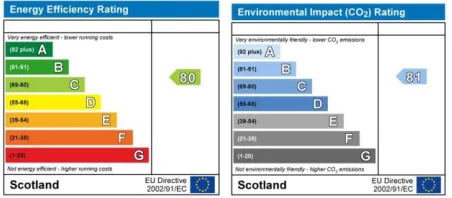
The buildings industry uses the SAP methodology to calculate a rating for Energy Efficiency and Environmental Impact of that specific dwelling. The SAP methodology does not currently allow for advanced controllability of systems to be modelled. In order to achieve this, a simplified mathematical model is required with enough detail to know which factors are affecting the controllability. The rationale of IDEAS is to initially use a linear thermodynamic model with the non linearities associated with power limitations such as there is no cooling system.

2.1 Inverse Dynamics in Microsoft Excel

The fundamental difference in the approach taken in this dynamic model is the use of inverse dynamics. The use of inverse dynamics allows for the perfect control at each model timestep. At each timestep there is no need to solve an iterative or numerical process. By using inverse dynamics, the value at each model timestep is known. This is very powerful and also allows us to put dynamic simulation in Microsoft Excel.

Figure 3 – Inverse Dynamics; the Control System calculates the input required for a desired input Without this formula for inverse dynamics it would be impossible to place this model in Microsoft Excel. Inverse dynamics is an enabler, which allows IDEAS results to be calculated at each timestep. Detailed Dynamic Tools are a complex unfamiliar

3.0 METHODOLOGY

3.1 Building Physics and Mathematical Model

A fundamental building physics model was created to represent heat transfer between the dwelling and the outside environment. The differential equations were derived from first principals. Once differential equations were created they were converted into state space for controllability analysis.

The proposed model is specifically developed to test the controllability of a dwelling. The dynamic model describes the energy and mass balance of air in the dwelling having a heating system. The assumptions inherent in constructing this model are numerous. However, the purpose of the model is not to emulate future reality and base design decisions around it, as advanced integrated software packages, such as ESPr (16) already exist.

The simplified model assumes that the indoor zone air is fully mixed at constant pressure and is stratified for natural ventilation. The dwelling glazing, roof and floor are considered to be in steady state, using U values taken directly from SAP. This leads to far less complex dynamic equations, but detailed enough to analyse controllability. At each timestep, the furniture & internal mass in the dwelling is modelled together in addition to the structure and air temperature.

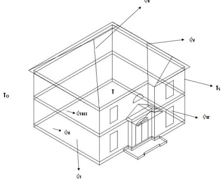
3.2 Heat Flow through the Dwelling

The walls of the dwelling are assumed to be a source of heat storage. The heat transfer is between the wall temperature and the internal temperature. Heat from external air is stored in the structure. When the temperature drops in the zone the heat is transferred into the room. In the same way when the wall temperature drops below the room temperature then heat is transferred to the wall.

It is assumed that the energy stored in windows, roof and floor are all negligible compared with the air mass and structure, such that:

Windows Heat Loss is: ( ( ) ( ))

w w w o

Q U A T t T t

(1)

Floor Heat Loss is: ( ( ) ( ))

F F F g

Q U A T t T t

(2)

1

Roof Heat Loss is: ( ( ) ( ))

R R R o

Q U A T t T t

(3)

Furniture and Internal Mass Heat Loss is: Q_FT U_FTA_FT( ( )T t T_FT( ))t

(4)

The above equations state that there is constant heat loss through windows, furniture and internal mass, roof and floor and thus these building elements are always in steady state condition. This assumption fits with U-Values and their use in SAP. The heat loss through a solid wall is approximated by one energy store, the thermal mass of the bricks and the overall U Value for conductions through the wall. The focus of the method is for a structure of uniform material; hence one node for Ts is used.

3.3 Rate of Change of Stored Heat

Thermal corner effects are neglected so that internal and external wall areas can be assumed the same. U-Values are used to model the heat transfer through the building fabric. While the thermal resistances and thermal capacities can be

calculated, a weighted average of these resistances and capacities was used for a single capacity equivalent of a multi-layer wall construction to simplify the model for controllability analysis.

The rate of heat stored in the bricks is:

( )

S STORED S S

dT t

Q

M C

dt

This also equates to the difference between the rate at which heat is entering and leaving the wall:

2

( ( )

( )) 2

(

( )

( ))

STORED S S S S S S o

Q

U A T t

T t

U A T t

T t

Where a factor of 2 in equation (6) is used to prevent the heat transfer being halved at steady state (10). Such that:

( )

( ( )

( ))

(

( )

( ))

2

S S S

S S S S S S o

M C dT t

U A T t

T t

U A T t

T t

dt

(7)

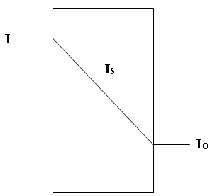
When the rate of change of the structure temperature (Ts) is zero (steady state mode assumes that the structural temperature of a dwelling is constant), SAP equivalent results should be produced. When the wall temperature has reached a steady state value, this as expected will be given by:

( ) ( ) ( )

2 o S

T t T t

T t (8)

Where TO is the external zone temperature connected to the wall, and T is the

temperature inside the dwelling; Heat Loss from the room:

( ) ( ) 2 ( )

2 o S S

T t T t U A T t

(9)

Steady State structure heat loss:

(

( )

( ))

Sss S S S o

Q

U A T t

T t

(10)

3.4 Rate of Change of Air Temperature

In IDEAS, we assume that air is highly stratified and fully mixed so that we have a constant temperature in the building. The air in the room is described as:

( )

( ) ( ) ( ) ( ) ( ) ( ) ( ) ( )

A A H FREE S F R W V FT

dT t

M C Q t Q t Q t Q t Q t Q t Q t Q t

dt (11)

Where Q_FREE( )t is free heat gain from: Appliances

People Lighting Solar Gain

For which normal SAP derived figures are updated so that real measured data is used, at a sampling resolution of 5 minutes. Climate data for Sheffield, UK was imported into IDEAS, using a data file from Meteonorm (17); this was used to provide a dynamic dataset for Solar Gain. Appliance Gains were taken from an International Energy Agency / Energy Conservation in Buildings and Community Systems

Program (ECBCS) Annex 42 study based upon real UK test data for 69 monitored dwellings (18). Metabolic Gains are calculated based upon the number of occupants in each particular dwelling. This figure is derived from the SAP provided Total Floor Area figure TFA. Lighting gains are taken into consideration in the Appliance Gains figure.

H

Q is the heating system under control and QVis from the natural infiltration

4.0 Controllability Analysis

The differential equations are factorised and simplified for controllability analysis. Temperature of Internal Dwelling Air:

( ( ) ( )) 2 ( ( ) ( )) ( ( ) ( )) ( )

( ( ) ( )) ( ( ) ( )) ( ( ) ( ))

H FREE V A o S S S F F o

A A

R R o w W o FT FT FT

Q Q M C T t T t U A T t T t U A T t T t

dT t M C

dt U A T t T t U A T t T t U A T t T t (12)

Temperature of Dwelling Structure: ( )

2 ( ( ) 2 ( ) ( )) S

S S S S S o

dT t

M C U A T t T t T t

dt (13)

Temperature of Dwelling Furniture & Internal Mass:

( )

( ( )

( ))

FT

FT FT FT FT a FT

dT

t

M C

U

A

T t

T

t

dt

To Simplify (14), the equation is factorised in terms of variables:Q_H, Q_FREE, T, TS , TFT and To:

11 12 13 11 11 12

( )

( )

( )

( )

( )

dT t

a T t

a T t

a T

t

b Q

d Q

d T t

dt

Where Constants are defined as follows:

11

12 13 11

11 12

2

2 1

1

V A S S F F R R w W FT FT

A A

S S FT FT

A A A A A A

V A F F R R w W FT FT

A A A A

M C U A U A U A U A U A

a

M C

U A U A

a a b

M C M C M C

M C U A U A U A U A

d d

M C M C

(16)

The same procedure of simplification is carried out for (Temperature of Dwelling Structure);

21 22 22

( )

( )

( )

( )

S

S o

dT t

a T t

a T t

d T t

dt

(17)

Where a21, a22 and d22 are given by:

21 22 22

2 S S 4 S S 2 S S

S S S S S S

U A U A U A

a a d

M C M C M C

(18)

The same procedure of simplification is carried out for (Temperature of Dwelling Furniture and Internal Mass);

31 33

( )

( )

( )

dT

t

a T t

a T

t

dt

31 33

FT FT FT FT

FT FT FT FT

U A U A

a a

M C M C (20)

4.1 State Space Model

In order to apply the aerospace controllability science (19), the mathematical model detailed in dynamic equations must be represented in State Space representation.

( ) ( ) ( ) ( )

x t Ax t Bu t Dd t (21)

Where (21) is the state equation, x t( )_{is the State Vector,} Ax t( )_{is the State Matrix,}

( )

Bu t _{is the Input Matrix and} Dd t( )_{is the Disturbances Matrix.} ( ) ( )

y t Cx t (22)

Where (22) is the output equation.

This state space model describes the dynamic behaviour of the building and its systems for a small amplitude perturbation δ about a steady state equilibrium

condition. Where y(t) is the measured output vector, x(t) is a vector of state variables, u(t) is a vector of system inputs (i.e. controller outputs) and d(t) is a vector of

disturbances. A, B and D are time invariant matrices consisting of constants which have been derived in the Controllability Analysis section of this paper. The linear statespace model (21) describes the dynamic behaviour of the dwelling for a small amplitude perturbation δ.

These two equations can be put together in state space form:

11 12 13 11 11 12

21 22 22

31 33

( ) ( )

( ) ( )

0 0 ( ) 0

( )

( )

0 ( ) 0 0 0

( ) FREE S H S o FT FT

T t a a a T t b d d

Q t

T t

a a Q t d

T t

T t

a a T t

T t

(23)

5.0 CONTROLLABILITY

The engineering science presented in this paper is based on ‘A Perfect Control Philosophy’. This philosophy aims to establish for a given design, if perfect control is feasible whilst maintaining stability for the closed loop control system. The value of this feasibility strictly is in allowing the designer to assess the ease in which perfect control could be achieved. The assumption is that the easier it is to achieve perfect control then in reality the easier the real system will be to control. The authors believe that is a sound and thorough philosophy to adopt to establish the controllability of a dwelling.

In order to estimate the energy required to maintain an ideal standard occupancy temperature and time profile (such as that defined by BREDEM), the dynamics of the system have to be inverted to establish what power input is required at a system time to achieve the target temperature. This requires the solution to PERFECT control, which can be obtained using RIDE (20) control algorithms. The RIDE Theory utilises Inverse Dynamics, firstly defining the system output in state-space form. A feedback control system can only control (i.e. track) what it feeds back as measured system outputs. Thus, to analyse the controllability of the measurements, they must be defined. In this case, if room temperature is the system output:

( ) ( )

( ) 1 0 0 S

FT

T T Y t

T

(25)

( ) ( )

Y t T t (26)

We assume the temperature is the air temperature.

Here, we control T, soY T. We are trying to measure and control the energy requirement of the Dwelling so that the demand temperature. To invert the static space model we can apply the perfect inverse control law RIDE (11):

1

( ) ( ) ( ) ( ) _eq( )

U t g CB v t y t U t (27)

Where equation (27) is the control algorithm where: ( )

U t = Heater demand, determined by the controller to maintain the required air temperature.

1

( )

g CB = Controller gain matrix where, g is the Global Scalar Gain. ( ) ( )

v t y t = Difference between what is required V, and what is measured and

outputted y (i.e the actual dwelling air temperature). ( )

eq

U t =This will provide extra help (it is an estimate) to the controller to calculate the

correct heater setting (i.e. U(t)), to raise the temperature of the air to the required level (V).

CB will tell the direction of the asymptotes, whilst CB inverse is used to align the asymptotes towards the stable region. In this proposed method, we wish to use controllability to align the direction of the asymptotes towards the negative real axis of the root locus. This is where the system is PERFECTLY controllable.

When a system is controlled perfectly with the RIDE control law, the closed loop system response is a perfect first order system such that:-

( ) ( ) 1 gt

Y t v t e (28)

Where:

Y(t) = measured output vector

v(t) = is the target room temperature.

As t , Y t( ) V t( ) (29)

Equation (29) states as the Temperature of the air in the dwelling tend towards infinity, the system output (the temperature of the air which varies with time) tends to the target room temp (which also varies with time).

5.1 System Response

1

g

Figure 7 – System Response: Step Response Profile

The step response profile demonstrates that we can assign the responsivity of the system, and therefore allow the system to integrate within the SAP environment. Parameter g is the system response, which can be entered in minutes, and v(t) is the target room temperature. 1

g

is the response time which has an effect – this is already built into SAP. BREDEM 12 records the Responsiveness of a Primary

Heating System (Rp) on scale from Fully Responsive (1) to Completely Unresponsive (0). Thus, we can use this relationship to back substitute into the control law as a prediction to take into account the system’s response characteristic. In this case let us assume that g is very large as in the case of a very powerful direct electric heating system. Thus the control law in this case is given by:

2

( ) ( ) ( ) 2 ( )

( ) ( )

( ) ( ) ( )

V A S S

A A S S S

F F R R w W

H

V A F F R R

FT FT FT FREE o

w W FT FT M C U A

gM C v t T t T t U A T t

U A U A U A U t Q t

M C U A U A

U A T t Q t T t

U A U A

(30)

6.0 IDEAS Implementation

Equation 30 could be dynamically solved by Dynamics Modelling such as ESP and IES. An IDEAS model, created in Microsoft Excel 2007 is used to solve Equation 30 symbolically. In IDEAS, the building physics is represented by three linear Ordinary Differential Equations; describing the Temperature of outside Air, Internal Air and Furniture & Internal Mass, which have been put into State Space form. Relating all the necessary parameters we have, we can use Inverse Dynamics to find out what instantaneous heat is required to meet a certain temperature. IDEAS is a linear model of the building, although the model as whole is non linear. For example, constraints are placed into the model for maximum and minimum heat which can be delivered into the dwelling. Therefore the discontinuities associated with plant saturation for example are modelled.

6.1 Optimum Start

Optimum Start is required for both our fast acting (direct acting electric heating) and slow acting (underfloor heating) systems. Optimum Start will adjust the start time of a heating system so that a heating setpoint is always met in time. To add Optimum Start to IDEAS, we compensate forQHmax. The rate of change of temperature T, which varies with time (t); described as follows:

11 12 13 11 11 12

( ) ( ) _S( ) _FT( ) _H( ) _FREE( ) _o( )

T t a T t a T t a T t b Q t d Q t d T t (31) Figure 6 – Output from IDEAS model;

Transient response highlight the tracking of a SAP daily setpoint on cold winters day

Tem

per

a

ture

C

For Optimum Start and Optimum Control of our heater, we want to run the Heater (Q_H) as hard as possible for as short a time as possible. Therefore:

max

H H

Q Q (32)

The bigger the heater, the bigger the Q_Hmaxand therefore the shorter the Optimum Start time will be. A bigger heater should be more responsive than a smaller heater. Introducing QH max into the responsivity analysis in SAP could help sizing of heater in a SAP framework. In IDEAS we record theQ_H maxof a heating system (in Watts) and the responsiveness of a heating system in hours, g.

For Optimum Start, we require the following:

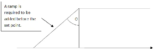
Figure 8 – Optimum Start Requirement

We cannot shift this to be generic as the size of a heating system and the value of g can differ (due to the responsiveness of a system), so the following is required:

Figure 9 – Optimum Start, addition of Ramp

The fundamental requirement of Optimum Start is to run the heating system at maximum power for as short as possible time.

For controllability of the system we break the system down into its fast and slow parts. Fast and Slow Decomposition of the Model:

11 max ( 11 ( ) 12 ( ) 13 ( ) 11 ( ) 12 ( ))

MAX H S FT FREE o

T b Q a T t a T t a T t d Q t d T t (33)

Where:

11 H max

b Q is the controllable ramp which is known.

11 12 13 11 12

Equation (33) sets a slope for our optimum start algorithm which is tracked by the heating system. The responsivity of the system is a combination of the amount of heat that can be delivered to the heater plus the effectiveness of the system itself (the systems time delay). Therefore a heater with an increased heat transfer for the same QH maxwill give a system with a higher responsiveness. It therefore could be possible to scale heating systems more accurately; a larger b₁₁term will give a more responsive system.

Due to the fast and slow decomposition of the model, in the time frame within the Optimum Start Period we can say that

. . . .. .

( ) S( ) FT( ) _FREE o( ) 0

T t T t T t Q T t (34)

We assume that the rate of change of the Free Heats, Outside, Furniture and Internal Mass, Air, and Structure is equal to Zero, due to the fast and slow decomposition of the model for this Optimum Start Period

We have two main properties of a heating system to compensate for:

1. The Maximum Power of the system

2. The responsiveness of the system - The g factor – how stable the control system could be

In the above method (equation (34)) we have compensated for the size of the plant relative to the building (the parameters of the building).

Figure 9 highlights our Optimum Start ramp to compensate for the maximum power of the heating system. We know what the optimum responsiveness of the system is, relative to the building. We need to compensate the slope based upon the thermal lag of the system. We therefore compensate for the phase lag which is the time constant of the system to react. We then shift the phase lag by 1/g to track the slope. This is the Steady State Tracking Error for a Ramp Input for a first order system (21). A first order system with a time constant lags a ramp at

1

to track the ramp you have to pass the ramp the time before equal to

1

underfloor heating, g will have to be set very low. And therefore the system will have to start a lot earlier for a defined set point to be achieved. The maximum g setting which can be used without the system going unstable is the maximum performance which can be produced from the Underfloor Heating system. A logical check is important in IDEAS to check that g is not infinity – if g was infinity then the optimum start time will be zero.

7.0 RESULTS

7.1 SAP Heating Profile

Figure 10 - BREDEM Weekday and Weekend heating profile for two zones (1)

Some coefficients in SAP are empirical and derived from extensive studies. The BREDEM Weekday and Weekend heating profiles for two zones are used to

determine the energy consumption of a dwelling. They are based upon temperature testing and recording of measured data of homes throughout the UK (Figure10). Monitored data was used extensively in the development of BREDEM.

7.2 Modelling a highly responsive system in IDEAS

A fast acting heating system consisting of a gas powered boiler and radiators was modelled in SAP and IDEAS.

The yearly SAP heating profile was tracked stating a temperature of 21°C in Zone 1 (Lounge) between 7 and 9am, and 4 and 11pm; Weekend heating profile states a Zone 1 temperature of 21°C being applied between 7am and 11pm (Figure 10). Figure 11 below highlights the transient performance of the IDEAS model, the setpoint is reached for the demand time, in keeping with the philosophy of SAP.

Figure 11 – IDEAS Optimum Start tracking of a SAP Setpoint for a fast acting heating system

The graph titled Optimum Start in figure 11 above highlights how similar the IDEAS setpoint with Optimum Start is to the SAP/BREDEM demand profiles in figure 10. Therefore with a heating system of a fast responsiveness, only a minimum Optimum Start is required.

7.3 Modelling a slow responsive system in IDEAS

A slow acting heating system consisting of an electrically supplied underfloor heating system was modelled in SAP and IDEAS. We can illustrate the effect of slow order systems by reducing the g term but a more accurate method would be to include the dynamics of the heating system within the model.

Tem

per

a

ture

C

Tem

per

a

ture

C

It can be seen from Figure 12 above that due to the slow responsiveness of this type of heating system an Optimum Start which varies significantly from that determined by SAP (figure 10) and calculated by IDEAS (figure 11) for a fast responsive system. Figure 12 details that for a slowly responsive system an Optimum Start requiring 21°, for almost 24 hours each day is required for the SAP demand heating profile to be met.

7.4 Optimum Start implementation findings and SAP Comparison

The implementation of Optimum Start into IDEAS has highlighted the variance in required Optimum Start by heating systems of differing responsiveness. This work could also be used to assist with determining the likelihood of overheating in a dwelling based upon the responsiveness of a heating system.

An additional area where Optimum Start in IDEAS could benefit SAP is to determine if the sizing of a heating system is appropriate for a particular dwelling. Figure 13 below highlights an example of reachability where there is not enough power in the heating system for the demand profile to be met.

The IDEAS tool could be used to suggest what heating system would be most appropriate to a dwelling, base upon the specifics of that dwelling as required to determine the SAP rating of that dwelling.

8.0 Conclusion

This paper presents the current SAP methodology and the BREDEM foundations with respect to the Energy Estimation of a Heating System for a dwelling. From this a new methodology is presented based upon systems engineering analysis and control theory knowledge developed from the aerospace industry. The work

presented in this paper is an encouraging start and a foundation. The focus of this Figure 12 – IDEAS Optimum Start tracking of a SAP setpoint for a slow acting heating system

Tem

per

a

ture

C

Tem

per

a

ture

C

Day of the Week _Wednesday

Figure 13 – ‘Reachability’ demonstrated in IDEAS

Tem

per

a

ture

C

paper was the implementation of an optimum start algorithm into a simplified symbolic model.

An energy estimation model for a single zone dwelling was presented; the

methodology can be used to supplement the SAP Methodology. Currently SAP is linear; the net response at a given place and time caused by two or more stimuli is the sum of the responses which would have been caused by each stimulus

individually (22). We need Non Linear SAP to take into account the non linearity of the system. In reality, systems are not perfect and behave in a non-linear manner. For example, natural ventilation and radiation are both non linear. Heating Systems are not perfect and behave in a Non Linear method. For the SAP methodology to accurately model Non Linear systems such as Heating, a Non Linear method must be employed.

The methodology presented builds on the foundations set by BREDEM, by

highlighting the importance of Responsivity, Efficiency and Controllability factors of a system. These factors are very important in the aerospace industry in addition to the buildings industry, and therefore it is felt that the correlation between the two

sciences is appropriate.

The main benefits of this proposed addition to the SAP methodology are

advantageous to both the dwelling occupier and the environment. A dwelling with good control is a home which has good occupant comfort, saves energy and therefore also saves the occupier money. The reduction in energy use from a well controlled dwelling has a positive effect on both the dwellings SAP score and the environment. A dwelling with poor control wastes energy, can cause discomfort for the tenant and can increase dwelling CO2 emissions. Without the addition of

optimum start, the lack of controllability of heating systems would result in an increase in energy use and a poorer SAP rating.

8.1 Discussion and Future Work

The Dynamic model presented is a fundamental model based on the linearised thermodynamics of the dwelling. This can be extended to a non linear third order model. The philosophy is extendable to non-linear models and can include higher order models.

As highlighted in the conclusions, this work is a foundation focused on the example of a dwelling structure with a uniform material; this work will be taken further by building on the flexibility that this method offers. The method will be extended for composite wall types based upon a resistance – capacitance (R-C) model (23).

IDEAS is currently a linear model with constraints. Whilst this is a simple model, work is already being carried out on more sophisticated approaches to include a non linear model and also the actual specific dynamics of the heating system to further detail. The linear Ordinary Differential Equations are required to be replaced with Non Linear versions. QFree Gains and Weather Data is independent of model (whether model is linear or non-linear) and so this data will be still be usable in a future non linear physics model. Comparative studies between the current linear model and a non linear model would then be required.

framework (24). This work highlights the dwelling design versus dwelling

performance gap and the importance of rigour in methods such as SAP. New tools such as IDEAS can be an important part of this discussion and can suggest how SAP could evolve in the future.

Further analysis is required into the integration of the optimum start algorithm in respect of a wider number of dwelling heating sources, including renewables. The effect of optimum start on a dwellings energy use and temperature levels can also be researched further.

Acknowledgement

BRE TRUST for the funding of this research

References

1. Anderson BR, Chapman PF, Cutland NG, Dickson CM, Henderson G, Henderson JH, et al. BREDEM 12 - Model Description: BRE; 2001.

2. European Parliament. DIRECTIVE 2002/91/EC OF THE EUROPEAN PARLIAMENT AND OF THE COUNCIL of 16 December 2002 on the energy performance of buildings. Official Journal of the European Communities. 2003. 3. Cooper GA. SAP 2005 and Low Energy Dwellings: Oxford Brooks2008. 4. Reason L, Clarke A. PROJECTING ENERGY USE AND CO2 EMISSIONS FROM LOW ENERGY BUILDINGS; A COMPARISON OF THE PASSIVHAUS PLANNING PACKAGE (PHPP) AND SAP: AECB2008.

5. Murphy GB, Kummert M, Anderson B, Counsell J. A comparison of the UK Standard Assessment Procedure and detailed simulation of solar energy systems for dwellings. Journal of Building Performance Simulation. 2011;4(1):75-90.

6. Tashtoush B, Molhim M, Al-Rousan M. Dynamic model of an HVAC system for control analysis. Energy. 2005;30(10):1729-45.

7. Hudson G, Underwood C, editors. A simple building modelling procedure for MATLAB/SIMULINK1999.

8. Counsell JM, Khalid YA, Brindley J. CONTROLLABILITY OF BUILDINGS, A multi-input multi-output stability assessment method for buildings with slow acting heating systems. Simulation Modelling Practice and Theory. 2010.

9. Tindale A. Third-order lumped-parameter simulation method. Building Services Engineering Research and Technology. 1993;14(3):87.

10. Khalid Y. Controllability of Building Systems. Glasgow: Strathclyde; 2011. 11. Counsell JM. Optimum and safe control algorithm (OSCA) for modern missile autopilot design. . Lancaster: Lancaster University; 1992.

12. Uglow CE. Energy use in dwellings: An exercise to investigate the validity of a simple calculation method. Building Services Engineering Research and Technology. 1982;3(1):35.

13. Uglow CE. The calculation of energy use in dwellings. Building Services Engineering Research and Technology. 1981;2(1):1.

14. Anderson BR, Chapman PF, Cutland NG, Dickson CM, Doran SM, Henderson G, et al. BREDEM 8 - Model Description: BRE; 2001.

15. French MJ. Conceptual design for engineers: Springer Verlag; 1999. 16. ESRU. ESP-r Applications Tutorial. 2011 [2011/05/20]; Available from:

http://www.esru.strath.ac.uk/Programs/ESP-r_tut/esp_aps.htm.

17. Meteotest. Meteonorm - Global Meteorological Database version 6.1. 2011 [cited 2011 10/10]; Available from: www.meteotest.ch/en.

19. Bradshaw A, Counsell J. Design of autopilots for high performance missiles. ARCHIVE: Proceedings of the Institution of Mechanical Engineers, Part I: Journal of Systems and Control Engineering 1991-1996 (vols 205-210). 1992;206(29):75-84. 20. Muir E, Bradshaw A. Control law design for a thrust vectoring fighter aircraft using robust inverse dynamics estimation (RIDE). ARCHIVE: Proceedings of the Institution of Mechanical Engineers, Part G: Journal of Aerospace Engineering 1989-1996 (vols 203-210). 1989-1996;210(47):333-43.

21. Franklin GF, Powell JD, Emami-Naeini A. Feedback control of dynamic systems: Addison-Wesley Reading (Ma) etc.; 1994.

22. Bach DR, Flandin G, Friston KJ, Dolan RJ. Time-series analysis for rapid event-related skin conductance responses. Journal of neuroscience methods. 2009;184(2):224-34.

23. ISO E. 13790: 2008. Thermal performance of buildings-Calculation of energy use for space heating and cooling. 2008.