Stepwise Development and Verification of a Boiler System Specification

      

City, University of London Institutional Repository

Citation: Bishop, P. G., Burns, G. and Anderson, S. O. (1993). Stepwise Development and Verification of a Boiler System Specification. Paper presented at the International

Workshop on the Design and Review of Software Controlled Safety-related Systems, 28 - 29 Jun 1993, National Research Council, Ottawa, Canada.

This is the unspecified version of the paper.

This version of the publication may differ from the final published version.

Permanent repository link: http://openaccess.city.ac.uk/551/

Link to published version:

Copyright and reuse: City Research Online aims to make research outputs of City, University of London available to a wider audience. Copyright and Moral Rights remain with the author(s) and/or copyright holders. URLs from City Research Online may be freely distributed and linked to.

Stepwise Development and Verication of a Boiler System

_Specication

Peter Bishop and Glenn Bruns and Stuart Anderson

Abstract

The rigorous development and verication of a boiler system specication is presented. Part I shows how the boiler system controller can be developed in a series of elaboration steps in which variables that directly reect plant conditions are replaced by variables representing sensed, communicated values. Part II shows how the safety of the system can be assessed by rst verifying safety relative to some failure assumptions and then estimating the likelihood that the assumptions hold.

1 General Introduction

In attempting to demonstrate the safety of the Generic Boiler System, two main

problems are faced. First, there are a wide range of possible failures that can occur. For example, the physical devices themselves can fail, sensors can fail, and sensed values can be delayed or lost in transmission. Taking careful account of all possible failures is dicult. A second problem, common to all safety-critical systems, is that absolute safety cannot be shown. One can only hope to demonstrate partial or probable safety. However, estimates of the probability of safety are hard to calculate, and it is hard to know

whether one can place much condence in them.

The approach demonstrated here addresses both of these issues. We present a stepwise approach to the development of the boiler monitoring and control system. Initially, we present an idealised controller that observes plant variables directly. Successive steps make weaker assumptions, until nally we arrive at a specication in which only sensor values received from the data communications system are observed. At each step, safety of the boiler system is maintained. In this way, failures are treated systematically. The second part of our approach is a separation of the deterministic and probabilistic parts of the safety analysis. Safety is proved of the boiler system absolutely, under certain assumptions that are believed to nearly always hold. Next, the likelihood of these

Part 1 - Step-Wise Derivation of a Boiler System

_Specication

Peter Bishop, Adelard, UK

1 Introduction

This part intended to illustrate the value of a step-wise approach for the derivation and validation of a specication using the Generic Problem as an example.

The basic strategy is to start with a model of the plant. Initially we model the

unconstrained behaviour of the plant where the plant may exhibit any physically feasible behaviour. We then need to identify the permissible set of safe behaviours: the safety constraints and, for the successful working of the plant, we also need to identify the normal operating constraints (see gure 1).

Given these basic denitions we now need to consider how this top-level set of requirements is elaborated into a software specication. We do this by constructing successive models of the control system which can satisfy the top-level constraints. In considering the physical plant and equipment we need to model failures as well as ideal operation. In order to demonstrate safety at a given level we may require extra

assumptions that constrain the behaviour of that model. For example, it may be

necessary to assume that only a single failure will exist at any given time, or that failures are always detected. Obviously these assumptions are not always correct but we should be able to compute the probability of violating the design assumptions.

So nally we should be able to derive a specication of the software function that should satisfy the plant safety constraints provided the additional equipment-related

assumptions are true. We can then estimate the probability that the equipment-related assumptions are violated in order to determine whether the system meets some

quantitative safety target.

It should be noted that the main intent is to illustrate the basic step-wise approach and the reasoning behind the safety arguments. While the approach is expressed in a formal notation, it does not claim to be rigorous.

The paper will primarily consider the elaboration of the safety specication for a controller. However we shall also consider some aspects of the availability requirements which have relevance to the Generic Problem Specication.

2 Formal Notation Employed

Lamport's TLA (Temporal Logic Algebra) [2] is used as the formal notation to represent the boiler and control system behaviour. TLA can specify temporal formulae such as:

x

= 0^2

x

0=

x

+ 1. This would describe the a variable

x

that, on each transition step,

increments indenitely from a value of zero. The reader is referred to Part II of this paper for a description of the semantics of TLA.

2.1 Denitions and conventions

We userangesto represent most values because error and uncertainties need to be taken

into account. For example, a meter reading of

x

might be manipulated as a range (

x

;

err

min

;x

+

err

max). We also use the following notational conventions:

V

p The physical limits of a plant variable (usually xed).

V

m The measured value of a plant variable.

f

d The failure state of plant component

d

.

r

d The reported (diagnosed) failure state of plant component

d

.

Unless otherwise specied, ranges are normally represented by a single upper-case letter. For convenience, the instantaneous value of plant variable is regarded as a range i.e.

V

= (

v;v

) where

v

is the scalar plant value.

2.2 Range Operators

A range

A

is represented as a pair (

x;y

) in which

x

and

y

are real and

x

y

.

We dene some operations on ranges: (

x;y

)1

4

x

(

x;y

)2

4

y

A

B

4

A

1

B

1

^

A

2

B

2

A

+

B

4 (

A

1+

B

1

;A

2+

B

2)

A

;

B

4 (

A

1

;

B

2

;A

2

;

B

1)

3 Boiler System Safety Requirement

3.1 Dening the Plant Model

xed time intervals. The interval between time instants is arbitrary, but to make life easier, we shall interpret the successive instants as the plant interface sampling time points (5 second intervals). This is suciently small to capture most boiler dynamics, and simplies the equations used for the various levels of modelling.

In dening the plant behaviour we will use the following plant variables:

L

boiler content level

S

steam ow per unit time

D

drain ow per unit time

P

pump ow per unit time

np

number of operating pumps

t

the current time and the following constants:

Safe

p safe static boiler level range

Safe

safe shutdown level range (dynamic operation)

K

pump ow per pump

L

p physical limits of boiler level

P

p physical limits of net pump ow

S

p physical limits of steam ow

S

p physical limits on change of steam ow / unit time The boiler model is dened as:

Boiler

4

L

0=

L

+

P

0 ;

S

0 ;

D

0 ^

P

=

K

np

^

L

L

p ^

S

S

p ^

S

0

;

S

S

p ^

P

P

p ^

t

0

=

t

+ 1

The rst line of the denition is a mass balance equation where the change in level is the dierence between the input and output ows. Subsequent lines specify constraints on the physical values. The nal line models the passage of time for successive transitions. This is not strictly needed for the plant model, but is relevant to time-dependent denitions in the controller. It is included in the boiler model since it is a physical quantity.

For convenience, the maximum change in level

L

per unit time due to physical ow limitations is dened as:

Note that this denition excludes the drain valve ow

D

since this only appears to be used at system start-up, and there is no specication for the physical limits of the maximum drain ow.

It should be noted that Part 2 uses a reduced boiler model which excludes timing and the drain valve ow. However the models are equivalent under under the analysis

assumptions made in Part 2.

3.2 Establishing the Boiler System Safety Requirement

The plant model dened above can exhibit any arbitrary behaviour permitted by its denition. In practice we wish to constrain its behaviour to meet some operational criterion. The overall safety criterion for the boiler system is:

2LSafe p

where

L

is the boiler level, Safe

p is the physical range of levels for boiler safety.

At an abstract level we should be able to identify a `constraint behaviour' that can meet this criterion. We then have to show that, given some safe initial condition, this

constrained behaviour always satises the plant safety property.

A more restrictive set of behaviours can be dened for maintaining plant availability, but this not the major property of concern here. Some aspects of availability will be discussed later.

3.3 Identifying the Shutdown Safety Boundary

At the top level of implementation, we have to identify a suitable constraint behaviour. In the Generic Problem Specication, some form of shutdown action is taken. There is no information about how the boiler actually shuts down, but since the plant cannot

shutdown immediately, we have to establish another range

Safe

such that:

L

Safe

^2(

Boiler

^

ShutBehaviour

) ) 2

L

Safe

p

Where

ShutBehaviour

is some arbitrary shutdown behaviour. One rather unlikely example of

ShutBehaviour

could be:

ShutBehaviour

4 :(

L

Safe

) ) (

S

0= 0

^

P

0= 0

^

D

0= 0)

With this extremely idealized system, it is fairly clear that excursions will be halted one time step beyond the

Safe

region. Since the shutdown occurs in a single time step,

Safe

must satisfy:

where

L

p is the maximum change in level that is physically possible in one step. In practice, the shutdown behaviour would be more complex and there would have to be a greater margin between

Safe

and

Safe

p, i.e.:

Safe

+

L

Shutdown

Safe

p

but the same approach should be applicable. Note that the dynamic aspects of shutdown have already been taken into account in the Generic Problem Specication, so the

specied range of

Safe

is assumed to have been veried.

3.4 Partitioning the Control System

Having identied the shutdown safety boundary, we can consider the structure of control system to implement the safety and normal operation requirements. We can divide the control system into two parts: a system which implements the plant shutdown behaviour

PlantShutdown

, and a controller unit

Shutdown

which detects unsafe plant conditions and also performs normal plant control actions. These two components are connected by a signal

up

which is monitored by the

PlantShutdown

system. When the

up

signal is false the boiler shutdown behaviour is triggered.

We can now consider these two systems separately. In particular, we can construct a sub-model containing the

Boiler

model and the

ShutDown

model for which we wish to show that:

2up ) LSafe

Or in other words, whenever the signal true, there is a safe level in the boiler. Provided

up

is true initially, this specication, combined with the

PlantShutdown

specication should ensure the overall safety criterion is always satised.

3.5 Elaboration Strategy

We now need to elaborate the design of the controller. The requirements for normal operation are not considered, only those aspects relevant to safety, i.e. the value of

up

. The basic approach to the design is a re-denition of

Shutdown

in a sequence of design elaborations

i

. In the physical system hardware failures can occur, so we wish to ensure the system isfail-safe i.e. shutdown will occur if the boiler limits are exceeded or if the

controller fails. so we dene the abstract signal

up

to be implemented by:

up

4

up

i ^

ok

i

Where variable

ok

i is used to represent an acceptable physical failure status. and

up

i represents the safety limit check implemented in terms of information available at that level of elaboration. The implementation

BSys

i is dened as:

In producing that implementation we may also make a set of design assumptions

Assump

i. In order for the implementation to satisfy the abstract safety specication we have to show that:

BSys

i ^

Assump

i ) 2(

up

i ^

ok

i )

L

Safe

)

It will be seen that at each stage of elaboration, additional uncertainty (or `fuzz') is introduced regarding the water level position. It will also be seen that additional

assumptions have be made to accommodate the physical characteristics and failure modes of the various controller subsystems.

3.6 Elaboration 1 - Plant Measurement

Obviously in the physical implementation, measured values will be used rather than the true plant variables. This data acquisition process is modelled as:

Measure

4

t

m =

t

^ (:

f

l )

L

L

m) ^ (:

f

s )

S

S

m)

^ (:

f

p )

np

=

]i:

(

pm

i ^

pi

i)

where the

L

m and

S

m are nominal accuracy ranges,

pm

i and

pi

i are independent indications of whether pump

i

is on, and

f

l,

f

s and

f

p refer to the failure states of the respective sensors.

In the simplest case we can just take the measured level

L

m. In this case this it is clear that if

up

1=

L

m

Safe

then:

(:

f

l ^

up

1)

)

L

Safe

If

ok

1 =

:

f

l then the safety requirement is met. However the controller has no absolute

knowledge of device failure status: it has to rely on a reported failure status,

r

l, which is based on some (unspecied) diagnosis

Diag

l of the measured values, i.e.:

ok

1 = :

r

l

So we need an assumption:

Assump

1 4

f

l )

r

l

to obtain a valid value for

ok

1.

Like all assumptions, this may not be valid in practice, and the chance of the assumption being violated will have be evaluated probabilistically. So the overall denition for shutdown at this elaboration is:

ShutDown

1 4

Measure

^

Diag

l ^

up

1=

L

m

Safe

^

ok

3.7 Elaboration 2 - Data Fusion

For availability reasons, the Generic Problem requires operation to be maintained for as long as is safely possible using available data. In order to achieve this we require adata fusionapproach where of faulty measurements are diagnosed based on the consistency of

the measurements. This topic is quite complex and is discussed in detail in Part 2. However the general features of the data fusion process are:

A consistency model for measured values.

`Fusion' which identies all potentially failed devices (i.e./ the values of

r

l,

r

s,

r

p). A computation which utilizes the failure reports and measured values to compute a

bounding range,

L

c such that:

L

L

c

For convenience this whole process is termed the

FusionProcess

. With data fusion we have to assume that the failure of all the sensors are detectable. In addition, data fusion is probably impossible if there is ow through the drain valve (since it is not measured), so we assume:

Assump

2

4

f

l )

r

l ^

f

s )

r

s ^

f

p )

r

p ^

D

= 0

It is assumed that the fusion process can be characterized by a variable

FusionOK

, such that:

FusionOK

)

L

L

c

FusionOK

will be false when it is impossible to compute

L

c. One example of this is when the level measurement is initially faulty (

t

= 0^

r

l), in this case there is no basis

for extrapolation using the steam and pump ow measurements. So the overall shutdown denition is:

ShutDown

2

4

Measure

^

FusionProcess

^

up

2 =

L

c

Safe

^

ok

2 =

FusionOK

3.8 Elaboration 3 - Eect of Communications

The communications system can corrupt a message, so correct measurements are only received when there are no communications failures, i.e.:

where

f

x is the message corruption state. We assume there is sucient redundancy in the message to perform a diagnosis of a faulty message, i.e.:

f

x )

r

x

where

r

x is the diagnosis.

Loss of messages eectively increases the time between measurement samples, and hence the uncertainty in the current value of the level. In order to guarantee safety, we require an upper limit on the interval between valid messages,

t

x, otherwise the worst case change in level cannot be predicted, hence.

ok

3

4

ok

2

^ (

t

0

m;

t

)

t

x

where

t

m is the time of the last received message and

t

is the current time.

To detect the existence of valid messages, we need an extra assumption for this level:

Assump

3

4

Assump

2 ^

f

x )

r

x

Taking the worst case changes permitted by the physical constraints, the range of

possible values for the level will expand by:

L

p

t

x where

L

p is the maximum possible

change in level per unit time. Thus the denition of the shutdown function is:

ShutDown

3

4

Comms

^

FusionProcess

2 ^

up

3 =

L

c+

L

p

:

t

x

Safe

^

ok

3 =

ok

2

^(

t

m;

t

)

t

x

FusionProcess

2 is an extension of the original fusion process which takes account the variable communication delays.

3.9 Elaboration 4 - Computer System Hardware

Obviously computer hardware failures (represented by

f

h) will aect the safety behaviour. In terms of the available information the system has to rely on

r

h, the reported hardware failure status. Thus we can dene

ok

4 4

ok

3

^:

r

h

Hence we need to assume:

Assump

1 4

f

h )

r

h

in order to ensure that

ok

4 is valid.

So at this level of the elaboration, the controller is dened as:

ShutDown

4

4 :

f

h ) (

Comms

^

FusionProcess

) ^

up

4=

L

c+

L

p

:

t

x

Safe

^

ok

3.10 Summary of the Elaboration Sequence

The following table shows the evolution of the design. For each implementation

i

, (

ok

i ^

up

i) is necessary to avoid shutdown.

Model

ok

up

Assumptions

Ideal

true

L

Safe

ShutDown

1

:

r

l

L

m

Safe

f

l )

r

l

(measurement)

ShutDown

2

FusionOK

L

c

Safe

f

l )

r

l

(+fusion)

f

s )

r

s

f

p )

r

p

D

= 0

ShutDown

3

ok

2

^(

t

m;

t

t

x)

L

c+

L

p

t

x

Safe Assump

2

(+comms) ^

f

x )

r

x

ShutDown

4

ok

3

^:

r

h

L

c+

L

p

t

x

Safe Assump

3

(+computer) ^

f

h )

r

h

It should be noted that further work is required to complete the elaboration. In particular, the chain of communication of the

up

i signal to some physical actuation system has not been addressed.

4 Availability Considerations

5 Impact of Plant Failures

We now have to consider whether this control behaviour can prevent excursions when there are plant failures. The only physical plant failure is the failure of a pump, which can either be `stuck-on' or `stuck-o'. It can be shown from the engineering data that `bang-bang' control can only be maintained indenitely if there are no `stuck-on' pumps and only one `stuck-o' pump. What this means in physical terms is that if a pump is stuck-on and there is a low steaming rate, the water level keeps on rising until it hits the upper safety limit. Similarly if there are two stuck-o pumps, the pump ow may not keep up with the steaming rate so the water level can drop below the lower safety limit.

6 Comparison with the Generic Problem Specification

The Generic Problem Specication identies a number of states for the software

implementation. There are transition conditions between the states and certain specic control actions are required in each state. In order to make a comparison, we analysed the transition conditions in order to determine the `residence condition' and actions in each state. The residence condition is essentially the union of all the entry conditions, with all possible exit conditions removed. One feature that was noted when analysing the state transition diagram was the variation of entry conditions for the same node when entered from dierent source nodes. For instance, the `degraded mode' can be entered with all sensors working from the `normal mode', but with a sensor missing when entered from `emergency mode'.

The following features were observed this analysis:

there are `health checks' on the hardware which can prevent normal operation

altogether. This is similar to our initial condition, where the system must be

ok

^

up

before the system can operate.

If the checks are satisfactory, the safety limit check (similar to our

up

i) is applied in

all operational states using dierent data fusion methods. Limit excursions cause shutdown.

Assuming there is no limit violation, normal control actions are performed.

There are also transitions based on pump availability. This is directly related to our

availability analysis which shows that three pumps are required to maintain availability.

The `emergency' mode relates to the loss of the main level measurement, so some

form of data fusion is needed to calculate the current level.

maximum interval between messages.

6.1 Potential Problems

In reviewing this specication, a number of potential problems have been identied.

There is no recognition of the fact that a pump can be `stuck-on' since the Generic

Problem specication only includes fully usable pumps. As shown in the earlier availability analysis, continued availability cannot be guaranteed with a stuck-on pump. It might therefore be desirable to prevent start-up or immediately shut down when the condition is identied (as it does when there are less than three pumps working).

There is no information about what happens to the drain valve during operation.

In order to maintain safety and availability it is essential for the drain valve to be shut. There is no explicit control of this valve by the computer. Ideally it should only be possible to open it in the `system test mode', but nothing is specied.

The variation in the node entry conditions may indicate an inconsistency about

when to continue operating in the event of failures. Ideally there should be a set of invariant conditions for the safety of the plant after initialisation. The only aspect that might need to vary between modes is the operating status of the pumps.

7 Probabilistic Analysis

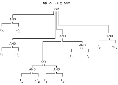
From the design assumptions and the modes of operation, we can construct a tree of failures leading to a dangerous failure (i.e. a failure to shut down when the level is potentially outside the safe limits). The actual structure of the tree will vary with the approach to data fusion. Figure 3 shows an example tree where the fusion relies on the level until it fails, then it uses the steam and pump ow measurements as an alternative. Provided the deterministic reasoning is correct, the top event can only occur when an assumption is violated. In our case, all these events are undetected failures, since detected failures can be rendered safe.

Provided we can assign probabilities to these base events, we should be able to compute the probability of the top event. To determine the probabilities we need to quantify:

the failure modes and failure rates of the sensors and the other hardware systems. the detection eciency of the diagnostic algorithms.

the repair time for reported failures. potential sources of common cause failure.

(1) There are many sources of common cause failure within the basic architecture because the control and shutdown functions both rely on

L

c. A better system design would have made the shutdown and control systems independent (e.g. independent sensors and hardware) so that there would be a higher probability of trapping control excursions (i.e. there is an AND at the top of the failure tree). (2) The communications system is one potential source of failure that aects all

measured variables and yet the specied protocol has no simple way of checking the integrity of the message. Reliance has to be placed on application-specic

knowledge (e.g. of the message contents, and credible values for variables). It would have been better if some standard message integrity check could be incorporated (e.g. CRC-32) whose diagnostic eciency is easily calculated for any specied level of `noise'.

(3) The level measurement is obviously very important since it is the main line of defence; the other variables are only signicant as standbys or consistency checkers. Safety and availability could be improved by the use of multiple level sensors.

8 Conclusions

The stepwise approach to the design allows the system to be reasoned about at a number of dierent levels. It allows the software specication to be related to specic features of the design which impinge on safety, and there is a logical connection with the

probabilistic safety analysis.

With regard to the Generic Problem Specication itself, many of the features derived by the stepwise analysis are analogous to features in the Problem Specication. However it was noted that certain aspects of the plant that could aect plant safety were not addressed, notably the control of the drain valve, and the treatment of `stuck-on' pump failures.

AAAA AAAA AAAA AAAA AAAA AAAA AAAA AAAA AAAA AAAA AAAA AAAA AAAA AAAA AAAA AAAA AAAA AAAA AAAA AAAA AAAA AAAA AAAA AAAA AAAA AAAA AAAA AAAA AAAA AAAA AAAA AAAA AAAA AAAA AAAA AAAA AAAA AAAA AAAA AAAA AAAA AAAA AAAA AAAA AAAA AAAA AAAA AAAA AAAA AAAA AAAA AAAA AAAA AAAA AAAA AAAA AAAA AAAA AAAA AAAA AAAA AAAA AAAA AAAA AAAA AAAA AAAA AAAA AAAA AAAA AAAA AAAA AAAA AAAA AAAA AAAA AAAA AAAA AAAA AAAA AAAA AAAA AAAA AAAA AAAA AAAA AAAA AAAA AAAA AAAA AAAA AAAA AAAA AAAA AAAA AAAA AAAA AAAA AAAA AAAA AAAA AAAA AAAA AAAA AAAA AAAA AAAA AAAA AAAA AAAA AAAA AAAA AAAA AAAA AAAA AAAA AAAA AAAA AAAA AAAA AAAA AAAA AAAA AAAA AAAA AAAA AAAA AAAA AAAA AAAA AAAA AAAA AAAA AAAA AAAA AAAA AAAA AAAA AAAA AAAA AAAA AAAA AAAA AAAA AAAA AAAA AAAA AAAA AAAA AAAA AAAA AAAA AAAA AAAA AAAA AAAA AAAA AAAA AAAA AAAA AAAA AAAA AAAA AAAA AAAA AAAA AAAA AAAA AAAA AAAA AAAA AAAA AAAA AAAA AAAA AAAA AAAA AAAA AAAA AAAA AAAA AAAA AAAA AAAA AAAA AAAA AAAA AAAA AAAA AAAA AAAA AAAA AAAA AAAA AAAA AAAA AAAA AAAA AAAA AAAA AAAA AAAA AAAA AAAA AAAA AAAA AAAA AAAA AAAA AAAA AAAA AAAA AAAA AAAA AAAA AAAA AAAA AAAA AAAA AAAA AAAA AAAA AAAA AAAA AAAA AAAA AAAA AAAA AAAA AAAA AAAA AAAA AAAA AAAA AAAA AAAA AAAA AAAA AAAA AAAA AAAA AAAA AAAA AAAA AAAA AAAA AAAA AAAA AAAA AAAA AAAA AAAA AAAA AAAA AAAA AAAA AAAA AAAA AAAA AAAA AAAA AAAA AAAA AAAA AAAA AAAA AAAA AAAA AAAA AAAA AAAA AAAA AAAA AAAA AAAA AAAA AAAA AAAA AAAA AAAA AAAA AAAA AAAA AAAA AAAA AAAA AAAA AAAA AAAA AAAA AAAA AAAA AAAA AAAA AAAA AAAA AAAA AAAA AAAA AAAA AAAA AAAA AAAA AAAA AAAA AAAA AAAA AAAA AAAA AAAA AAAA AAAA AAAA AAAA AAAA AAAA AAAA AAAA AAAA AAAA AAAA AAAA AAAA AAAA AAAA AAAA AAAA AAAA AAAA AAAA AAAA AAAA AAAA AAAA AAAA AAAA AAAA AAAA AAAA AAAA AAAA AAAA AAAA AAAA AAAA AAAA AAAA AAAA AAAA AAAA AAAA AAAA AAAA AAAA AAAA AAAA AAAA AAAA AAAA AAAA AAAA AAAA AAAA AAAA AAAA AAAA AAAA AAAA AAAA AAAA AAA AAA AAA AAA AAA AAA AAA AAA AAA AAA AAA AAA AAA AAA AAA AAA AAA AAA AAA AAA AAA AAA AAA AAA AAA AAA AAA AAA AAA AAA AAA AAA AAA AAA AAA AAA AAA Unsafe behaviour Safe behaviour

Set of all plant behaviours

[image:15.595.166.444.57.336.2]

Normal Constrained behaviour

Fig 1. Behaviour of Hazardous Plant

S

D P = K.np

L

Safe Safe_p

np

[image:15.595.169.430.405.672.2]

AND

f

h ¬ rh

OR

AND

f

l ¬ rl

AND

f

p ¬ r p

AND

f

s ¬ rs OR

AND

f_{l l}

AND AND

f

x ¬ rx

r ¬ L Safe⊆

[image:16.595.96.496.107.395.2]

up ∧

Part II | Verifying Properties of a Boiler System

Glenn Bruns and Stuart Anderson

Laboratory for Foundations of Computer Science University of Edinburgh

Edinburgh EH9 3JZ, UK

1 Introduction

To rigorously show that a safety-critical system is safe, one would like to take advantage of the many existing system verication techniques. Unfortunately, this cannot be done, at least directly, because no real system is absolutely safe | there is always at least a remote chance that a component will fail. However, it is not necessary to reject logical techniques in favour of wholly probabilistic ones. In this paper we show that the safety of systems can be proved, relative to failure assumptions that hold only in a probabilistic sense.

We demonstrate our approach by proving safety and other properties of a generic boiler system [

?

], composed of a boiler, feed pumps, sensors, and a monitoring and control system. We formally specify the plant and monitoring sub-systems, and show that the system as a whole is safe relative to failure assumptions that state, for example, that if all monitored values are consistent, in a precise sense, then no device has failed. We also show some important failure reporting properties of the system.

2 Notation

We will use Lamport's Temporal Logic of Actions (TLA) to describe both the boiler system and its properties. We briey describe TLA here; for more details see [

?

]. The atomic formulas of TLA are predicates and actions. A predicate is a boolean expression build from variables and values, such as

x >

1. A predicate can be regarded semantically as a function from states to booleans, where a state is a mapping from variables to values. An action is a boolean expression built up from variables, primed variables, and values, such as

x

0=

x

+ 1. An action can be regarded semantically as a

relation on states, in which primed variables refer to a \new" state and unprimed

variables to an \old" state. Thus,

x

0=

x

+ 1 holds between two states if the value of

x

in

the new state is one greater than the value of

x

in the old state.

The syntax of TLA formulas is as follows, where

P

ranges over predicates andA ranges

over actions:

F

::=

P

2A :

F F

1

^

F

2

A TLA formula is valid if it is satised by every innite sequence of states. Predicate

P

is satised by sequence

if

P

holds for the rst state of

. Action Ais satised by

if A

holds for the rst pair (

s

0

;s

1) of states in

. Formula

:

F

is satised by

if

F

is not

satised by

. Formula

F

1 ^

F

2 is satised by

if both

F

1 and

F

2 are satised by

.

Finally,2

F

is satised by

if

F

is satised by every sux of

.

Systems are always represented in TLA by formulas of the form

P

^2A, where

P

represents an initial condition. For example, (

x

= 0)^2(

x

0=

x

+ 1) represents a system

in which

x

is initially 0 and is incremented in every successive state. To express the correctness condition that a property

F

holds of a system Sys, we write Sys)

F

. For

example, letting Sys be the formula

x

= 0^2(

x

0=

x

+ 1), we write Sys

)2(

x

0

> x

) to

express that

x

increases in every successive state of Sys.

Some basic TLA proof rules, taken from [

?

], are listed in Appendix

??

.

In modelling the boiler system it is convenient to have variables that represent a range of values. For example, we model the measured boiler level as a range that takes the

possible measurement error into account. All model variables of type range have names beginning with an upper-case letter. Formally, a range is a pair (

x;y

) in which

x

and

y

are real and

x

y

. We dene some operations on ranges:

(

x;y

)1 def

=

x

(

x;y

)2 def

=

y

A

B

def

=

A

1

B

1 and

A

2

B

2

A

[

B

def

= (min(f

A

1

;B

1

g)

;

max(f

A

2

;B

2

g))

A

+

B

def

= (

A

1+

B

1

;A

2+

B

2)

A

;

B

def

= (

A

1 ;

B

2

;A

2 ;

B

1) j

A

j

def

=

A

2 ;

A

1

Notice that ranges are closed under the;operator. We will later use the fact that + and ;are monotonic with respect to, so that

A

B

)(

A

+

C

)(

B

+

C

), and similarly

for the; operator.

For convenience, certain plant variables that really represent scalar values are also represented as ranges of the form (

x;x

).

3 Modelling the Boiler System

We now present a formal model of the boiler system, based on [

?

]. Roughly, our model contains a part that models the physical plant and a part that species a plant monitor. The plant monitor does not explicitly contain modes, but does perform the failure

emergency, and shutdown modes of operation. We model sensors and sensor failure, but do not model data communications. Also, we do not model the boiler control scheme; the safety properties we prove hold for any control scheme.

We begin by describing the model variables. Our specication contains the following plant variables:

L

boiler content level

S

steam ow per unit time

np

number of operating pumps

L

m metered content level

S

m metered steam ow rate

pi

i motor on/o indicator for pump

i

pm

i monitor for pump

i

the following control variables:

L

c calculated boiler content level

S

c calculated steam rate

P

c calculated net pump rate

f

d actual failure of device

d

r

d reported failure of device

d

c

D consistency of readings from devices in set

D

up

shutdown variable

and the following constants:

L

p physical limits of boiler level

S

p physical limits of steam ow

P

p physical limits of net pump ow Safe safe boiler level range

K

pump ow per pump

The subscript

d

of variables

f

d and

r

d range over elements of Devdef

= f

l;s;p

g, where

l

stands for the content level meter,

s

stands for the steaming valve meter, and

p

stands for the pumps. In writing a consistency variable

c

D, we abbreviate device sets as strings of symbols from Dev, for example, we write

c

sp instead of

c

fs;pg.

model states the relationships between physical plant variables, and also contains failure assumptions:

Boiler def

=

L

0

=

L

+ (

P

0 ;

S

0

)

^

P

=

K

np

^

S

S

p ^

P

P

p

^ :

f

l)

L

L

m ^ :

f

s)

S

S

m ^ :

f

p)

np

=

]i:pm

i

^ ^

d2Dev 0 @

f

d ) _

Dfdg :

c

D

1 A

^ ^

DDev 0 @

:

c

D ) _

d2D

f

d

1 A

The model is a discrete approximation of the physical plant behaviour. The rst three failure assumptions state that the meters are accurate in the absence of failure. The fourth states that failure of a device

d

produces some inconsistency involving

d

. The nal assumption states that every inconsistency is produced by some failed device.

We use the notationV

i2I

F

i rather than

8

i

2

I:F

i because we always quantify over nite

sets, and are therefore using only simple propositional logic, not predicate logic. The notation

]i:F

i denotes the number of

i

for which

F

i holds.

The shutdown model determines the value of the variable

up

, which holds whenever the calculated boiler level is within the safe bounds:

Shutdown def

=

up

=

L

c

Safe

The data fusion model determines the value of failure reporting variables. The model states that if an inconsistency exists for some device set

D

, then all devices in

D

are reported as failed. This pessimistic failure reporting strategy is necessary when calculating a level range that is guaranteed to contain the actual boiler level.

Fusion def

= ^

d2Dev 0 @

r

d = _

Dfdg :

c

D

1 A

Notice that the failure reporting strategy is given as a function of consistency conditions only.

The consistency model states consistency conditions between device readings. Informally,

meter reading taken alone is consistent, i.e., if it is not outside the possible physical range. Similarly,

c

sp holds if the steam and pump readings are consistent. Note that

:

c

d

1d2 does not imply :

c

d

1 or :

c

d

2.

Cons def

=

c

s=

S

m

S

p ^

c

p =8

i:pm

i =

pi

i ^

c

l =

L

m

L

p ^

c

sp = true ^

c

sl= true ^

c

pl = true ^

c

0

spl =

L

0

m

L

m+ (

K

(

]i:pm

0

i);

S

0

m)

The nal component determines the estimated level variable from reported failures. The calculated level is the best estimate of the actual level given the current reported failure conditions. For example, if the level meter is not reported as failed, then the best estimate of the actual level is by the level meter.

Level def

= :

r

0

l)

L

0

c =

L

0

m

^

r

0

l)

L

0

c =

L

c+ (

P

0

c;

S

0

c)

^ :

r

s)

S

c=

S

m ^

r

s)

S

c =

S

p

^ :

r

p)

P

c=

K

(

]i:pm

i) ^

r

p )

P

c =

P

p

The action Step represents the combined behaviour of the preceding components: Step def

= Boiler^Shutdown^Fusion^Cons^Level

The initial conditions include the conjunct

L

c =

L

, which states that we must initially know the actual level of the boiler.

Init def

=

L

c=

L

^

L

Safe

The top-level boiler system description has the standard form of a TLA specication: BSys def

= Init^2Step

4 Failure Properties

failure occurs it should be reported. This is critical to the proof of safety. Letting

D

r be the the set of devices reported as failed, and

D

f be the set of actually failed devices, the property can be formalised as follows:

Pessimismdef

= 2(

D

f

D

r)

Theorem 1

BSys)Pessimism

Proof.

_D

f =f

d

2Devj

f

dg by denition of

D

f

f

d) W

Dfdg

:

c

D in def. of Boiler

D

f f

d

2Devj W

Dfdg

:

c

Dg propsitional logic, set theory

D

f f

d

2Devj

r

dg by denition of

r

d

D

f

D

r by denition of

D

r

Clauses of Step were used to prove

D

f

D

r, so by the deduction principle we have that

Step)

D

f

D

r. TLA rule STL4 then gives us that2Step) 2(

D

f

D

r), and from

this BSys)Pessimismeasily follows. 2

The second property is that if one or more devices are reported as failed, then at least one of the reported devices must have actually failed. This property can be formalised as follows:

No False Alarmsdef

= 2(

D

r6=;) _

d2D r

f

d)

Theorem 2

BSys)No False Alarms

Proof.

By denition,

D

r =f

d

2Devj

r

dg. Expanding the denition of

r

d and

simplifying, we equivalently have that

D

r =S

f

D

Devj:

c

Dg. Writing the nitely

many elements of the setf

D

Devj:

c

Dgasf

D

1

;:::;D

n

g, we have that

D

i

D

r and

thatW

d2D

i

f

d for 1

i

n

. Therefore, since

D

r6=;, W

d2D r

f

d.

2

5 Safety Properties

The most important property to show is that if the shutdown variable

up

is true, then the boiler level is within its safe bounds. This notion of safety can be formalised in TLA as the formula:

Safetydef

= 2(

up

)

L

Safe)

Before proving the safety property we present a few lemmas. Of these, the third is the most important, stating that the actual boiler level is always within the calculated level range.

Proof.

Assume that Step holds. If :

r

s then

S

c =

S

m. By the Pessimism property we

know that:

r

s):

f

s, and since :

f

s)

S

S

m, we have

S

S

c. If

r

s, then

S

c

S

p, and

since

S

S

p, we have

S

S

c. Thus Step)

S

S

c. 2

Lemma 2

Step)

P

P

c

Proof.

We use a similar argument as in the proof to the previous theorem. If :

r

p, then

P

c =

K

(

]i:pm

i) and

np

=

]i:pm

i, so

P

c=

P

. If

r

p, then

P

P

c just as for

r

s. 2

Lemma 3

BSys)2(

L

L

c)

Proof.

To simplify the proof, we use the following derived TLA proof rule (where

I

is a predicate):

A)

Q I

^(A^

Q

0)

)

I

0

I

^2A)2

I

To see that the rule is sound, observe that we get2A)2(A^

Q

0) from the rst premise

by TLA rule STL4 and other rules of simple temporal logic, and that we get

I

^2(A^

Q

0)

)2

I

from the second premise and TLA rule INV1. Putting these together

gives the conclusion.

We dene

R

to be (:

r

l):

f

l)^(

S

S

c)^(

P

P

c). The rst conjunct is a clause of

Step, and the others were shown to be implied by Step in the previous lemmas, so Step)

R

.

We now show that (

L

L

c)^(Step^

R

0)

)(

L

L

c) 0. If

:

r

0

l, then

L

0

c =

L

0

m by a clause of Level. Knowing:

r

0

l also gives us:

f

0

l, by a conjunct of

R

0, and therefore

L

0

L

0

m, giving

L

0

L

0

c. If

r

0

l, then

L

0

c =

L

c+ (

P

0

c;

S

0

c). By

L

L

c,

R

0, and since + and ;are

monotonic on ranges, we have that

L

+ (

P

0 ;

S

0)

L

c+ (

P

0

c;

S

0

c), so

L

0

L

0

c. Applying the derived proof rule we get (

L

L

c)^2Step)2(

L

L

c). Furthermore,

L

L

c holds initially, giving Init^2Step)2(

L

L

c). 2

Theorem 3

BSys)Safety

Proof.

BSys ) 2Step by def. of BSys ) 2(

up

)

L

c Safe) by def. of Shutdown

BSys ) 2(

L

L

c) Lemma

??

BSys ) 2(

up

)

L

Safe) by TLA rule STL5 and trans. of

6 Failure Assumptions and Consistency Conditions

We have shown some important safety properties of the boiler system relative to some failure assumptions. As mentioned in the Introduction, the probability that the

assumptions hold could be estimated, allowing an overall estimate of system safety to be made. We will not perform a probabilistic analysis here, but will review the failure assumptions we have made and the related consistency conditions.

First, we have assumed that devices report values within their specied accuracy when they have not failed. Estimating the likelihood of this condition holding would probably be possible.

Second, we have assumed that failed devices report inconsistent values. Calculating the likelihood of this assumption holding is likely to be dicult, as a detailed knowledge of the likelihood and behaviour of failure modes is needed. Furthermore, the system context is relevant. For example, a meter that fails to a 0 reading will produce a consistent failure in contexts where a 0 reading is expected.

Third, we have assumed that inconsistencies arise only in the presence of failures. The diculty of assessing this assumption depends on the particular consistency conditions adopted.

The consistency conditions play no part in the deterministic analysis, but do aect the probabilistic analysis. The conditions chosen in our model could certainly be augmented. For example, the conditions

c

p and

c

lcould be strengthened by additionally requiring that the change in pump and level values in the last step are within a certain range. The condition

c

spl holds when the level meter reading is consistent with the old level reading and the calculated net ow. Note that this condition depends on values in both the current and previous states. The use of values from the current and previous state in determining consistency could be extended so that a sequence of past values is used. For example, a sequence of ow values could be recorded and tested. An important part of the design of the boiler system is the selection of consistency conditions that are easy to compute and likely to uncover device failures. Furthermore, a good consistency condition is one for which it is possible to estimate the probability that the condition fails just when some device fails.

7 Conclusions

if level meter ok then

L

c:= level meter reading

else if steam meter ok then

S

c := steam meter reading else

S

c := physical steam limit

if pump mon's ok then

P

c := sum of pump mon. readings else

P

c := sum of physical pump limits

L

c :=

L

c+ (

P

c;

S

c)

Figure 1: The Level Calculation in Pseudo-code

inadequate to ensure the main safety property.

The process of proving the properties was also benecial. Attempting the proofs often uncovered missing details, such as initial conditions. On the other hand, superuous parts of the specication were found by examining the nished proofs, and noting the dependencies on the specication. For example, we had initially included a single-failure assumption in the model, and realised later, after looking at our proofs, that this

assumption was not needed.

Some parts of the model are generic and could be used for other systems. The data fusion model embodies a general strategy for detecting failure from inconsistencies between measured values. We chose a pessimistic strategy that reports a device failed if a

measurement from the device is inconsistent with other values. Less pessimistic strategies may be better in other contexts. For example, another strategy is to select the smallest set of devices such that some device in the set is guaranteed to have failed. Thus if the

:

c

spl and :

c

pl, the devices

p

and

l

might be reported as failed, but not

s

. Failure

assumptions could also be incorporated into data fusion model, allowing a smaller set of devices to be reported as failed. For example, if:

c

sp and:

c

sl, and if

f

l implies :

f

s and :

f

p, then one can conclude that

s

has denitely failed.

The level calculation strategy is also quite generic. This strategy is related to various software fault-tolerance schemes, such as recovery blocks [

?

,

?

]. The resemblance may be easier to see if the strategy is given in pseudo-code (see Figure

??

) rather than in logic. In a recovery block, alternative computations are tried until an acceptable result is delivered. Here, alternative computations are ordered according to the accuracy of the result. A specic computation is chosen according to which devices have failed.

Acknowledgements

Appendix A Some TLA Proof Rules

STL1

F

provable by propositional logic

F

STL2 `2

F

)

F

STL3 `22

F

2

F

STL4

F

)

G

2

F

)2

G

STL5 `2(

F

^

G

)(2

F

)^(2

G

)

STL6 `(32

F

)^(32

G

)32(

F

^

G

)

INV1

P

^A)

P

0

P

^2A)2

P

Appendix B Bibliography

[1] T. Anderson and P.A. Lee, editors. Fault Tolerance: Principles and Practice. Prentice Hall, 1981.

[2] Specication for a software program for a boiler water content monitor and control system. Institute for Risk Research, 1992.

[3] Leslie Lamport. The temporal logic of actions. Technical Report 79, Digital Systems Research Center, 1991.