Fatigue life prediction on nickel base superalloys

Full text

(1)University of Southampton Research Repository ePrints Soton. Copyright © and Moral Rights for this thesis are retained by the author and/or other copyright owners. A copy can be downloaded for personal non-commercial research or study, without prior permission or charge. This thesis cannot be reproduced or quoted extensively from without first obtaining permission in writing from the copyright holder/s. The content must not be changed in any way or sold commercially in any format or medium without the formal permission of the copyright holders.. When referring to this work, full bibliographic details including the author, title, awarding institution and date of the thesis must be given e.g. AUTHOR (year of submission) "Full thesis title", University of Southampton, name of the University School or Department, PhD Thesis, pagination. http://eprints.soton.ac.uk.

(2) University of Southampton School of Engineering and Applied Sciences Materials Research Group. Fatigue Life Prediction of Nickel Base Superalloys by Mark Miller. Thesis Submitted for the degree of Engineering Doctorate July 2007.

(3) University of Southampton Abstract School of Engineering and Applied Sciences Materials Research Group Engineering Doctorate. Fatigue Life Prediction of Nickel Base Superalloys By Mark Miller Neural networks have been used extensively in material science with varying success. It has been demonstrated that they can be very effective at predicting mechanical properties such as yield strength and ultimate tensile strength. These networks require large amounts of input data in order to learn the correct data trends. A neural network modelling process has been developed which includes data collection methodology and subsequent filtering techniques in conjunction with training of a neural network model. It has been shown that by using certain techniques to ‘improve’ the input data a network will not only fit seen and unseen Ultimate Tensile Strength (UTS) and Yield Strength (YS) data but correctly predict trends consistent with metallurgical understanding. Using the methods developed with the UTS and YS models, a Low Cycle Fatigue (LCF) life model has been developed with promising initial results. Crack initiation at high temperatures has been studied in CMSX4 in both air and vacuum environments, to elucidate the effect of oxidation on the notch fatigue initiation process. In air, crack initiation occurred at sub-surface interdendritic pores in all cases. The sub-surface crack grows initially under vacuum conditions, before breaking out to the top surface.. Lifetime is then dependent on initiating pore size and distance from. the notch root surface. In vacuum conditions, crack initiation has been observed more consistently from surface or close-to-surface pores - indicating that surface oxidation is in-filling/”healing” surface pores or providing significant local stress transfer to shift initiation to sub-surface pores. Complementary work has been carried out using PWA 1484 and Rene N5. Extensive data has been collected on initiating pores for all 3 alloys. A model has been developed to predict fatigue life based upon geometrical information from the initiating pores. A Paris law approach is used in conjunction with long crack propagation data. The model shows a good fit with experimental data and further improvements have been recommended in order to increase the capability of the model..

(4) Contents. 1 Introduction...................................................................................................................1 1.1 Neural Networks for Fatigue Life Prediction.................................................................1. 2 Neural Network Design and Architecture....................................................................3 2.1 What is a Neural Network?.............................................................................................3 2.2 McCulloch-Pitts Neuron .................................................................................................3 2.3 Perceptron........................................................................................................................3 2.4 Multi-layer perceptron....................................................................................................5 2.5 Backpropagation..............................................................................................................5 2.6 Early stopping..................................................................................................................6 2.7 Fitting and over-fitting.....................................................................................................6 2.8 Regularization..................................................................................................................7 2.9 Other types of network....................................................................................................7 2.10 Analysis of Significance of Inputs...............................................................................10 2.11 Neural Networks to Predict Material Properties.......................................................10 2.11.1 Summary of Literature............................................................................................................14. 3 Fatigue.........................................................................................................................17 3.1 Introduction to Fatigue..................................................................................................17 3.2 Total Lifetime Approaches............................................................................................17 3.3 Introduction to Fracture Mechanics.............................................................................18 3.3.1 Linear Elastic Fracture Mechanics............................................................................................18. 3.4 Initiation of fatigue cracks.............................................................................................22 3.5 Stage I / II / III crack growth........................................................................................22 3.6 Extrinsic shielding effects (closure mechanisms).........................................................23 3.7 Short crack behaviour...................................................................................................24 3.8 Creep and Environmental Interactions........................................................................25 3.9 Creep-Fatigue.................................................................................................................25. 4 Nickel Based Super Alloys..........................................................................................27 4.1 Development of Nickel Based Alloys.............................................................................27 4.2 Microstructure...............................................................................................................27 4.3 Deformation of Nickel Base Alloys................................................................................28 4.4 Single Crystals................................................................................................................28 4.5 CMSX-4..........................................................................................................................29 4.5.1 Microstructure and Physical Properties.....................................................................................29 4.5.2 Heat Treatment..........................................................................................................................30 4.5.3 Oxidation behavior....................................................................................................................30 4.5.4 Creep.........................................................................................................................................31 4.5.5 Fatigue Behaviour.....................................................................................................................31.

(5) 4.5.6 Summary of CMSX-4 findings.................................................................................................32. 5 Neural Network Modelling.........................................................................................37 5.1 Program of Work...........................................................................................................37 5.2 Software Approaches.....................................................................................................38 5.2.1 Neuromat Overview..................................................................................................................38 5.2.2 Bayesian learning......................................................................................................................39 5.2.3 Ranking models.........................................................................................................................40 5.2.4 Data Preparation........................................................................................................................40 5.2.5 Training models.........................................................................................................................40 5.2.6 Committees of models...............................................................................................................41 5.2.7 Significance of inputs................................................................................................................41 5.2.8 Neuromat Notation....................................................................................................................42 5.2.9 Matlab........................................................................................................................................44. 5.3 Initial Modelling Work using UTS Database...............................................................48 5.4 Data Collection Methodology........................................................................................48 5.4.1 Data Sources..............................................................................................................................48 5.4.2 Selection of Inputs.....................................................................................................................49 5.4.3 Alloy composition.....................................................................................................................49 5.4.4 Processing parameters...............................................................................................................50 5.4.5 Heat Treatments........................................................................................................................51. 5.5 Predictions using UTS_IW7_Test database.................................................................52 5.6 Supporting work using Matlab.....................................................................................56 5.7 Summary of Preliminary Results..................................................................................58 5.8 Data Preparation and Analysis.....................................................................................59 5.9 Modifications to database..............................................................................................62 5.10 Models Using refined UTS Database..........................................................................64 5.10.1 Discussion..............................................................................................................................75 5.10.2 Conclusions ............................................................................................................................77. 5.11 YS database..................................................................................................................79 5.12 Statistical analysis of YS input database....................................................................79 5.13 Results from models trained on ‘clean’ YS dataset...................................................81 5.13.1 Supporting Work with Matlab Neural Network Models.........................................................86. 5.14 Discussion......................................................................................................................90 5.15 Conclusion....................................................................................................................91 5.16 Low Cycle Fatigue Model............................................................................................92 5.16.1 Introduction.............................................................................................................................92 5.16.2 Selection of inputs and data collection....................................................................................93 5.16.3 Analysis of Input Data.............................................................................................................94 5.16.4 Statistical Analysis..................................................................................................................97 5.16.5 Preliminary models..................................................................................................................99 5.16.6 Discussion.............................................................................................................................100 5.16.7 LCF model 2nd attempt.........................................................................................................101 5.16.8 Discussion.............................................................................................................................106. 5.17 Final Conclusions.......................................................................................................107. 6 Fatigue testing...........................................................................................................109 6.1 Introduction..................................................................................................................109 6.2 Materials.......................................................................................................................110 6.3 Material Characterisation...........................................................................................111 6.3.1 Sample preparation..................................................................................................................111.

(6) 6.3.2 Hardness testing......................................................................................................................112 6.3.3 Oxidation Study.......................................................................................................................112 6.3.4 Sectioning and Ni Plating........................................................................................................113 6.3.5 Porosity Analysis.....................................................................................................................113. 6.4 Finite Element Model...................................................................................................114 6.4.1 CMSX-4 Model geometry.......................................................................................................114 6.4.2 Elastic model - (determination of notch depth).......................................................................114 6.4.3 Elasto-plastic model - (evaluation of notch root stress/strain fields)......................................115 6.4.4 Sub-sized CMSX-4 specimens................................................................................................115 6.4.5 René N5...................................................................................................................................115 6.4.6 PWA 1484...............................................................................................................................115. 6.5 Fatigue Testing.............................................................................................................116 6.5.1 Specimen Preparation..............................................................................................................116 6.5.2 Testing Procedure....................................................................................................................117 6.5.3 Fractography............................................................................................................................118. 6.6 Results...........................................................................................................................124 6.6.1 Material Characterisation........................................................................................................124 6.6.1.1 Macrostructure.................................................................................................................124 6.6.1.2 Microstructure.................................................................................................................125 6.6.2 Oxidation Studies....................................................................................................................125 6.6.2.1 CMSX-4..........................................................................................................................125 6.6.2.2 ReneN5............................................................................................................................126 6.6.2.3 PWA1484........................................................................................................................126 6.6.2.4 Summary..........................................................................................................................127 6.6.3 Fatigue Testing Results...........................................................................................................127 6.6.3.1 Fatigue Test Lifetimes.....................................................................................................127 6.6.3.2 Fracture Surface Overviews............................................................................................129 6.6.3.3 Detailed Fractography – .................................................................................................131 CMSX-4 Tests in Air.............................................................................................................131 CMSX-4 Tests in Vacuum.....................................................................................................133 René N5 Tests in Air.............................................................................................................133 PWA1484 Tests in Air...........................................................................................................134 6.6.3.4 Collection of Porosity Data.............................................................................................134. 6.7 Discussion & Analysis of Results.................................................................................175 6.7.1 Fatigue Life Data.....................................................................................................................175 6.7.2 Fractography............................................................................................................................175 6.7.3 Analysis of porosity initiating fatigue cracks..........................................................................177 6.7.4 Effect of shape of initiating porosity.......................................................................................178 6.7.5 CMSX-4 long crack data.........................................................................................................178 6.7.6 Lifing Model............................................................................................................................179 6.7.6.1 Sensitivity to Pore Geometry...........................................................................................181 6.7.6.2 Sensitivity to Paris Constants and K level at failure.......................................................182 6.7.6.3 Fatigue life model results................................................................................................183 6.7.7 Fatigue life modeling using Neural Networks........................................................................183 6.7.7.1 Training a Neural Network to emulate the lifing model.................................................184 6.7.7.2 Training a Neural Network on test data...........................................................................184. 6.8 Discussion......................................................................................................................199 6.8.1 Fatigue life modeling...............................................................................................................200. 6.9 Conclusions...................................................................................................................203. 7 Final Conclusions ....................................................................................................204 8 Further Work.............................................................................................................206 Appendices. 207. References. 217.

(7) Figures Figure 1 - McCulloch - Pitts Neuron..............................................................................15 Figure 2 - A single neuron..............................................................................................15 Figure 3 - A basic network..............................................................................................15 Figure 4 a typical feed forward network.........................................................................16 Figure 5 An example of overfitting (after Neuromat reference manual)........................16 Figure 6 Evolution of yield stress as a function of temperature.....................................16 Figure 7 Evolution of creep rupture stress as function of temperature..........................16 Figure 8 - Anatomy of a Jet Engine................................................................................33 Figure 9 - Fir tree root fixing for turbine blade.............................................................33 Figure 10 - A typical S-N curve......................................................................................33 Figure 11 - Sharp crack length 2a in a thin elastic plate, with a nominal applied stress σ......................................................................................................................................34 Figure 12 - Sharp crack length 2a in an elastic plate, with a nominal applied stress σ 34 Figure 13 - Typical opening modes.................................................................................35 Figure 14 - Typical da/dN versus ∆K curve....................................................................35 Figure 15 - Typical long crack/short crack behaviour (after Suresh218)......................35 Figure 16 - Cuboidal γ'...................................................................................................36 Figure 17 - Cross-slip pinning mechanism, the dislocation cross-slips onto (010) due to lower APB energy and is locked in this configuration....................................................36 Figure 18 - Definition of secondary orientations A and B and their nominal crack growth directions.............................................................................................................36 Figure 19 Examples of two possible data fits (after Neuromat reference manual)........43 Figure 20 Addition of test data to indemtify model overfitting (after Neuromat reference manual)............................................................................................................................43 Figure 21 Effect of complexity (number of HU’s) on test and training error................43 Figure 22 – Test error vs. number of models in a committee.........................................43 Figure 23 – Example of Matlab output during training..................................................46 Figure 24 – Example of test vs training error graph generated using Matlab...............46 Figure 25 – Example of Matlab neural network predictions vs. actual data..................46 Figure 26 – Example of Significances related to input weights generated by Matlab. . .47 Figure 27 – Excel calculations for solution heat treatment approximation...................52 Figure 28 - UTS predictions for Nim739 using UTS_IW7_Test.....................................53 Figure 29 - UTS predictions for M313 using UTS_IW7_Test........................................54 Figure 30 - Comparison of data for Nim739 and IN939 + Neuromat prediction..........54 Figure 31 - Significance of inputs for best TE committee...............................................55 Figure 32 - Significance of inputs for best LPE committee............................................55.

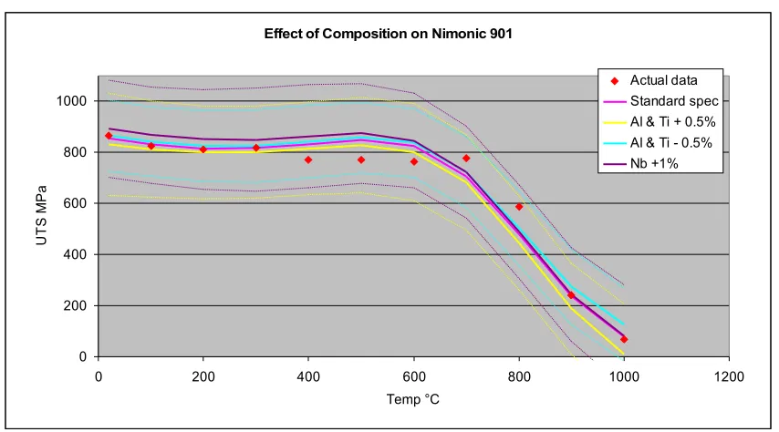
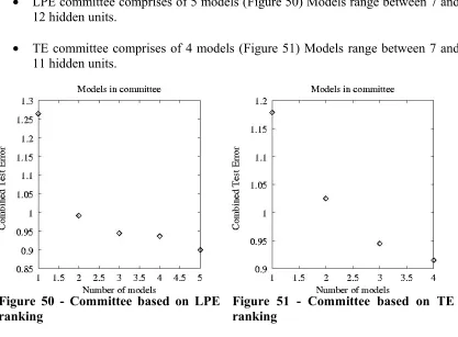
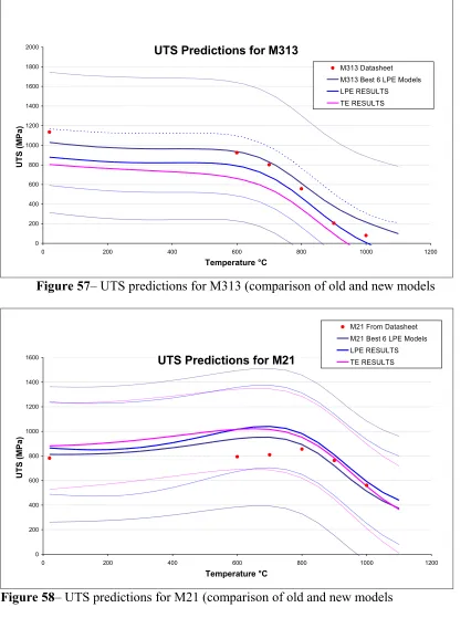
(8) Figure 33 – Models trained using the same training in Matlab using different initial values...............................................................................................................................56 Figure 34 – Predictions for Nim739 UTS, varying number of HU’s..............................57 Figure 35 – Full spread of UTS data by alloy (UTS vs. Temp)......................................61 Figure 36 – Identification of outliers in UTS database..................................................62 Figure 37 – Material curve for alloy R44.......................................................................62 Figure 38 – Data for U720 exhibiting large amounts of scatter at common test temperatures....................................................................................................................62 Figure 39 - Committee based on LPE ranking...............................................................64 Figure 40 - Committee based on TE ranking..................................................................64 Figure 41 – Neuromat predictions for Inconel 617 UTS................................................65 Figure 42 – Neuromat predictions for Nimonic 901 UTS...............................................65 Figure 43 – Neuromat predictions for MERL 76 UTS....................................................66 Figure 44 – Significance of inputs for input dataset UTS_17_01_05.............................67 Figure 45 – Sensitivity of UTS model to change in heat treatment for Inconel 617.......67 Figure 46 - Sensitivity of UTS model to change in 1st age temperature for MERL 76. .68 Figure 47 - Sensitivity of UTS model to change in 2nd age temperature for MERL 76. 68 Figure 48 Sensitivity of UTS model to change in 1st age temperature for Nimonic 90169 Figure 49 Sensitivity of UTS model to change in composition for Nimonic 901............69 Figure 50 - Committee based on LPE ranking...............................................................70 Figure 51 - Committee based on TE ranking..................................................................70 Figure 52 – Predictions for Inconel 617 using models trained with and without the test data set............................................................................................................................71 Figure 53 - Predictions for MERL 76 using models trained with and without the test data set............................................................................................................................71 Figure 54- Predictions for Nimonic 901 using models trained with and without the test data set............................................................................................................................72 Figure 55 – Significance values for UTS model committees..........................................72 Figure 56 – UTS predictions for Nimonic 739 (comparison of old and new models.....73 Figure 57– UTS predictions for M313 (comparison of old and new models..................74 Figure 58– UTS predictions for M21 (comparison of old and new models....................74 Figure 59 – Spread of data in UTS database for IN718.................................................78 Figure 60 – Input data spread for Cr in the YS database...............................................79 Figure 61 – YS database. All inputs with respect to test temperature...........................80 Figure 62 – YS prediction for Inconel 617 (seen data)...................................................81 Figure 63 YS prediction for MERL 76 (seen data).........................................................81 Figure 64 YS prediction for CMSX-4 (unseen data).......................................................82 Figure 65 YS prediction for Nimonic 901 (seen data)....................................................82.

(9) Figure 66 – significance of inputs for YS model.............................................................83 Figure 67 – Sensitivity to inputs YS model – CMSX-4 example......................................84 Figure 68 - Sensitivity to inputs YS model – MERL 76 example.....................................84 Figure 69 Significance of YS input values after training with 90/10 split......................85 Figure 70 Sensitivity to inputs YS (90/10 split) model – CMSX-4 example...................85 Figure 71 –YS predictions for M313 with 10 networks all using different seed points in Matlab.............................................................................................................................86 Figure 72–YS predictions for M22 with 10 networks all using different seed points in Matlab.............................................................................................................................87 Figure 73 - YS predictions for M21 with 10 networks all using different seed points in Matlab.............................................................................................................................87 Figure 74 – Effect of number of hidden units on model data fit (YS dataset) M22 alloy used as example...............................................................................................................89 Figure 75 – Total input space (strain range vs. cycles to failure) for LCF database.....94 Figure 76 – Spread of training data for Haynes 230 by strain range............................95 Figure 77 Spread of training data for Haynes 230 by test temperature and Ref source. .........................................................................................................................................95 Figure 78 Multi-plots -spread of training data for Haynes 230 by test temperature and reference source..............................................................................................................96 Figure 79 – PWA1480 strain life data............................................................................97 Figure 80 – Distribution of LCF model variables 1.......................................................98 Figure 81 – Distribution of LCF model variables 2.......................................................98 Figure 82 – LCF model predictions against unseen CMSX-4 data................................99 Figure 83 – LCF model significance of inputs..............................................................100 Figure 84 - Analysis of strain range distribution.........................................................100 Figure 85 – Matlab neural network demonstrating data fit to CM186 data................101 Figure 86 – LCF model predictions for seen data Haynes 230....................................102 Figure 87 – Neuromat LCF predictions for seen data CMSX-4...................................103 Figure 88 – Input significances for model trained on reduced input dataset...............103 Figure 89 – Neuromat LCF predictions for seen data CM186LC R=-1......................104 Figure 90 – Matlab LCF predictions for seen data CM186LC R=-1...........................104 Figure 91 – Neuromat LCF predictions for seen data CM186LC R=0.05...................105 Figure 92 – Matlab LCF predictions for seen data CM186LC R=0.05 (Key as in Figure 91)..................................................................................................................................105 Figure 93 – Ni plating apparatus..................................................................................120 Figure 94 - Meshing, loading and constraint strategy. Note distributed constraints shown (used in elasto-plastic model only) (after Mark Joyce).....................................120 Figure 95 - Notch root mesh detail – 8 node mapped quadrilaterals employed to accurately assess notch root fields (after Mark Joyce).................................................120.

(10) Figure 96 - Mode I stresses and strains predicted at notch root in CMSX-4 at 650°C. (after Mark Joyce).........................................................................................................121 Figure 97 – Stress/strain behaviour for PWA1480.......................................................121 Figure 98 - Abaqus FEA model of PWA 1484 test bar with detail of mesh refinement around notch root..........................................................................................................122 Figure 99 - Definition of secondary orientations A and B and their nominal crack growth directions...........................................................................................................122 Figure 100 - Secondary orientation with relation to dendrites taken from end of cast bar.................................................................................................................................123 Figure 101 - Short crack test specimen geometry.........................................................123 Figure 102 - Etched and polished notch (orientation B)..............................................123 Figure 103 - Trapezoidal 1-1-1-1 waveform.................................................................123 Figure 104 CMSX-4 dendrites (100) orientation.........................................................140 Figure 105 PWA1484 dendrites (100) orientation......................................................140 Figure 106 - René N5...................................................................................................140 Figure 107 SEI Image...................................................................................................140 Figure 108 Rhenium Concentration..............................................................................140 Figure 109 - Example of interdendritic porosity in RenéN5........................................140 Figure 110 Sample of porosity in CMSX-4 used for porosity analysis ........................141 Figure 111 – Example of FBTA cell gathering for CMSX-4 porosity..........................141 Figure 112 CMSX-4 - Slip bands around a hardness indent........................................141 Figure 113 PWA1484 - Slip bands around a hardness indent......................................142 Figure 114 CMSX-4 etched surface {001} orientation using FEG-SEM.....................142 Figure 115 SEM images Etched surface (left) Backscattered electron image (right) 111 plane..............................................................................................................................142 Figure 116 SEM image Etched surface of René N5 γ matrix (110) orientation A .......143 Figure 117 SEM image Etched surface of PWA1484 γ matrix (110) orientation A.....143 Figure 118 SEM images – Polished CMSX-4 after 1 hour exposure at 650°C...........144 Figure 119 SEM images – Polished CMSX-4 after 256 hours exposure at 650°C......145 Figure 120 SEM images – Polished and etched CMSX-4 after 1 hour exposure at 650°C.............................................................................................................................146 Figure 121 SEM images – Polished and etched CMSX-4 after 1 hour exposure at 650°C.............................................................................................................................147 Figure 122 SEM image - Slice from oxidised sample showing oxide thickness...........148 Figure 123 SEM image – As Figure 122, higher magnification...................................148 Figure 124 - Preferential oxidation of γ‘on an polished sample of Rene N5..............149 Figure 125 - oxidised carbides on Rene N5 oxidation sample (1)................................149 Figure 126 - oxidised carbides on Rene N5 oxidation sample (2)................................149 Figure 127 - - - oxidised carbides on Rene N5 oxidation sample (3)...........................149.

(11) Figure 128 Orientation A, Air, 21°C............................................................................150 Figure 129 Orientation A, Air, 650°C .........................................................................150 Figure 130 Orientation B, Air, 650°C..........................................................................150 Figure 131 Orientation B Air, 725°C...........................................................................151 Figure 132 Orientation B, Vac, 650°C.........................................................................151 Figure 133 Orientation A, Vacuum, 725°C..................................................................151 Figure 134 Orientation B Vacuum, 725°C...................................................................152 Figure 135 CMSX-4 Bar 16 OA....................................................................................153 Figure 136 CMSX-4 Bar 17 OB....................................................................................153 Figure 137 CMSX-4 Bar 24 OB....................................................................................153 Figure 138 CMSX-4 Bar 28 OB....................................................................................153 Figure 139 CMSX-4 Bar 29 OB....................................................................................153 Figure 140 René N5 Bar 1 OB......................................................................................154 Figure 141 René N5 Bar 2 OB......................................................................................154 Figure 142 René N5 Bar 3 OB......................................................................................154 Figure 143 René N5 Bar 4 OA......................................................................................154 Figure 144 René N5 Bar 5 OA......................................................................................154 Figure 145 René N5 Bar 6 OA......................................................................................154 Figure 146 BAR P28-A, OB..........................................................................................155 Figure 147 BAR P28-B, OB.........................................................................................155 Figure 148 BAR P24-A, OB..........................................................................................155 Figure 149 BAR P22-B, OB..........................................................................................155 Figure 150 BAR P22-A, OB..........................................................................................155 Figure 151 BAR P26-A, OB..........................................................................................155 Figure 152 – Strain Life data for all fatigue tests.........................................................156 Figure 153 SEI micrograph - Bar 1 - Orientation X, Fracture surface (a)..................157 Figure 154 SEI micrograph Interdendritic surface pore identified as major initiation point as marked on Figure 153.....................................................................................157 Figure 155 SEI micrograph of Pore on surface of etched notch from CMSX-4 room temperature test.............................................................................................................157 Figure 156 SEI micrograph Example of fracture surface features...............................158 Figure 157 Bar 2 - SEI micrograph overview Bar 2 orientation X, Air, 650°C, 100,000 cycles.............................................................................................................................158 Figure 158 SEI micrograph - Blemish observed on notch surface after testing at 650°C .......................................................................................................................................158 Figure 159 SEI micrograph - Large penetrating crack in oxide layer observed on notch surface after testing at 650°C.......................................................................................159 Figure 160 SEI micrograph image – As Figure 159 side on........................................159.

(12) Figure 161 BEI Topographical Scan of cracks in notch root oxide layer....................159 Figure 162 SEI micrograph of cracks in notch root oxide layer..................................159 Figure 163 SEI micrograph of cracks in notch root oxide layer..................................160 Figure 164 SEI micrograph – Fracture surface overview ,OA, 725°C, Air, 5271 cycles. .......................................................................................................................................160 Figure 165 SEI micrograph – Crack in notch surface (Figure 164 location A)...........160 Figure 166 SEI micrograph – Subsurface ‘halo’ crack initiation point (Figure 164 location B).....................................................................................................................161 Figure 167 SEI micrograph Sub-surface initiation point Orientation B, 650°C, 1-1-1-1, 6,500 cycles...................................................................................................................161 Figure 168 - SEI micrograph Subsurface initiation point Orientation A, 725°C.........161 Figure 169 - SEI micrograph Subsurface initiation point Orientation A, 725°C.........161 Figure 170 - BEI Topographical Scan. Sub-surface initiation point Orientation A, 725°C.............................................................................................................................161 Figure 171 - BEI Compositional Scan. Sub-surface initiation point Orientation A, 725°C.............................................................................................................................161 Figure 172 - EDX plot for Nickel, from Figure 171.....................................................162 Figure 173 - EDX plot for Oxygen, from Figure 171...................................................162 Figure 174 - EDX plot for Nickel, from Figure 171.....................................................162 Figure 175 - EDX plot for Nickel, from Figure 171.....................................................162 Figure 176 - EDX plot for Titanium, from Figure 171.................................................162 Figure 177 - EDX plot for Chromium, from Figure 171..............................................162 Figure 178 - EDX plot for Silicon, from Figure 171....................................................162 Figure 179 - EDX plot for Aluminium, from Figure 171..............................................162 Figure 180 - EDX plot for Tungsten, from Figure 171.................................................163 Figure 181 SEI micrograph crack propagation in CMSX-4 OA..................................163 Figure 182 SEI micrograph crack propagation in CMSX-4 OB..................................164 Figure 183 – Detail of sectioning and location of Figure 184, Figure 187Figure 185Figure 186...............................................................................................................164 Figure 184 SEI micrograph (Location A) oxide layer in notch root............................165 Figure 185 SEI micrograph (Location B) Crack following a slip band, cutting through g’....................................................................................................................................165 Figure 186 SEI micrograph (Location C) Crack deviation around pore before continuing along slip band............................................................................................165 Figure 187 SEI micrograph (Location D) oxide layer on fracture surface exhibiting ‘rooftop’ faceting...........................................................................................................166 Figure 188 – SEI micrograph fracture surface overview 650°, OB, Vacuum..............166 Figure 189 SEI micrograph – initiation pore 650°, OB, Vacuum................................166 Figure 190 SEI micrograph – initiation pore 650°, OA, Vacuum................................167.

(13) Figure 191 SEI micrograph – initiation pore 650°, OA, Vacuum................................167 Figure 192 SEI micrograph – Slip bands, pore and striations, 650°, OB, Vacuum.....167 Figure 193 SEI micrograph – Fast fracture region with porosity, 650°, OB, Vacuum168 Figure 194 SEI micrograph – initiation pore 650°, OA, Vacuum................................168 Figure 195 SEI micrograph overview – René N5 ffracture surface OA, 650°C, Air....169 Figure 196 - SEI micrograph Initiation site A (Figure 195).........................................169 Figure 197 - SEI micrograph Detail of initiating pore from Figure 196.....................169 Figure 198 - SEI micrograph Initiation site B (Figure 195).........................................169 Figure 199 - SEI micrograph Detail of initiating pore from Figure 198.....................169 Figure 200 - SEI micrograph Initiation site C (Figure 195)........................................170 Figure 201 - SEI micrograph Detail of initiating pore from Figure 200.....................170 Figure 202 - SEI micrograph Initiation site D (Figure 195)........................................170 Figure 203 - SEI micrograph Detail of initiating pore from Figure 202.....................170 Figure 204 Rene N5 fracture surface overview, OB.....................................................171 Figure 205 - SEI micrograph at location A (Figure 204).............................................171 Figure 206 - SEI micrograph at location B (Figure 204).............................................171 Figure 207 - SEI micrograph at location D (Figure 204)...........................................171 Figure 208 - SEI micrograph at location E (Figure 204).............................................171 Figure 209 - SEI micrograph at location C (Figure 204)............................................172 Figure 210 - SEI micrograph Detail of C (Figure 204)................................................172 Figure 211 - SEI micrograph orientation B with Nf of 3325 cycles ............................172 Figure 212 - SEI micrograph orientation B with Nf of 3507 cycles.............................172 Figure 213 Overview of fracture surface Bar P26-A, Orientation B, Nf = 182001.....172 Figure 214 SEI micrograph of the major initiation site in region A (Figure 213).......172 Figure 215 SEI micrograph at initiating facet region A (Figure 213).........................173 Figure 216 SEI micrograph detail of the dark phase in Figure 215 (possible oxidised carbide) that initiated first crack..................................................................................173 Figure 217 - Overview of fracure surface Bar P26-A, Orientation B, Nf = 182001:...173 Figure 218 SEI micrograph overview of the major initiation site in region A (Figure 217)................................................................................................................................173 Figure 219 - SEI micrograph of the initiation site in region A (Figure 217) ..............173 Figure 220 - SEI micrograph of initiating pore in Figure 219.....................................173 Figure 221 Pore measurement details..........................................................................174 Figure 222 Pore area calculation using TAP software ...............................................174 Figure 223 – Comparison of Southampton data with Alstom test data........................188 Figure 224 – Sum area of initiating pores vs. cycles to failure....................................188 Figure 225 – Major initiating pore vs. cycles to failure...............................................189.

(14) Figure 226 - effect of a/c ration on effective Kd (a simple analysis using Scott and Thorpe)..........................................................................................................................189 Figure 227 - CMSX-4 Long Crack Data (after Mark Joyce220)..................................190 Figure 228 Orientation A, Air fracture surface (after Mark Joyce220).......................190 Figure 229 Orientation A, Vacuum fracture surface (after Mark Joyce220)...............191 Figure 230 – Crack measurements for S&T analysis – OX 650°C air.........................191 Figure 231 – BAR OA, 725°C, Air, 5271 cycles...........................................................191 Figure 232 – Schematic of crack propagation from subsurface pore...........................192 Figure 233 Stress fieled in notch root of CMSX-4 notch bend bar...............................192 Figure 234 – Flow chart for Notch Fatigue Model.....................................................192 Figure 235 - Interaction plot for a, c and d with respect to subsurface life................193 Figure 236 - Interaction plot for a, c and d with respect to total life...........................193 Figure 237 – Surface plot for relationship between a, c and total cycles to failure.....194 Figure 238 – Surface plot for relationship between a, d and total cycles to failure.....194 Figure 239 – Correlation between predicted internal life and total predicted cycles to failure............................................................................................................................194 Figure 240 – Average effects for change in material properties vs cycles to failure for an average sized pore....................................................................................................195 Figure 241 – Interactions plot for mvac, mair, Cvac, Cair, Kcrit Vs. Cycles to failure .......................................................................................................................................195 Figure 242 – Power law fits in Excel to long crack data supplied by Mark Joyce.......196 Figure 243 - Predicted results vs. actual test results for 8mm x 8mm CMSX-4 Notch Bend Bars......................................................................................................................196 Figure 244 – Predicted results vs. actual test results (Large data points = main initiating pore, small data points = all other initiating pores for each bar)................196 Figure 245 – Training vs target data for 4 HU neural network using results from fatiue lifing model....................................................................................................................197 Figure 246 – Training error for neural networks using 1-20 HU’s.............................197 Figure 247 - Training vs target data for 3 HU neural network. Inputs = Material and Sum Area.......................................................................................................................197 Figure 248 - - Training vs target data for 3 HU neural network. Inputs = Material, Sum Area and Strain Range..................................................................................................198 Figure 249 – Significance of inputs for 3 HU model in Figure 248.............................198 Figure 250 - Training vs target data for 3 HU neural network. Inputs = Material, Sum Area, Test Temperature and Strain Range....................................................................198.

(15) Acknowledgements I would like to thank QinetiQ for the sponsorship of my Engineering Doctorate. The financial support of EPSRC is also gratefully acknowledged. Thanks also go to Alstom Power and GE for supply of raw materials. Thanks are extended to my academic tutor Dr Philippa Reed and colleague Dr Mark Joyce (University of Southampton) and industrial tutors Ian Wilcock and Dr Irene Di Martino (QinetiQ) for their support and guidance. I would also like to thank Dr Xijia Wu (CNRC Canada), Dr Mark Joyce, Amira Kawar and Irene Lee (University of Southampton) for their contributions to this work. Finally special thanks to my fiancée Nicky and my academic tutor Dr Philippa Reed who showed great patience as I procrastinated over my final write up and without whom I would have certainly have never finished..

(16) Nomenclature and Acronyms σ. ' f. -. Fatigue strength coefficient. -. Fatigue ductility coefficient.. -. Potential energy of an un-cracked plate. ∏. -. Potential energy supplied by internal strain energy and external forces. ϒe. -. Surface energy of the material. ε. ' f. ∏. 0. σf ϒp. -. Fracture stress Plastic work term. σy. -. Yield stress. ε. −. Strain. E. -. Elastic modulus. E. -. Energy. J. -. J integral. K. -. Stress intensity factor. KIC. -. Fracture toughness (mode I). Kth. -. Threshold stress intensity factor. Nf. -. Number of cycles to failure. -. Nv Ws. Valence-electron concentration -. APB ARD BEI CRP CRS DOE DS EDM EDX EPSRC FBTA FCC FEA FEG HCF HU LCF LEFM LPE MLP. Work required to create new surfaces.. -. Anti Phase Boundary Automatic Relevance Determination Backscattered Electron Image Collaborative Research Project Creep Rupture Strength Design of Experiments Directionally Solidified Electronic Discharge Machining Energy Dispersive X-ray Engineering and Physical Sciences Research Council Finite Body Tessellation Analysis Face Centre Cubic Finite Element Analysis Field Electron Gun High Cycle Fatigue Hidden Unit Low Cycle fatigue Linear Elastic Fracture Mechanics Log Predictive Error Multi Layer Perceptron.

(17) MSE NN NRC. -. Mean Squared Error Neural Network National research council (Canadian partners in CRP). OA OB ORT OX PM PX QQ RMS RR SEI SEM SEN SENB SSE SX TE UTS YS. -. Orientation A Orientation B Orientation Orientation X Powder Metallurgy Polycrystalline QinetiQ Root Mean Square Rolls Royce Secondary Electron Imaging Scanning Electron Microscope Single Edge Notch Single Edge Notch Bend Sum Squared Error Single Crystal Test Error Ultimate Tensile Strength Yield Stress.

(18) Alloys CM247 CMSX-4 IN939 Inconel 617 M21 M313 MERL 76 Nim739 Nimonic 901 PWA 1480 PWA 1484 U720. Cannon-Muskegon alloy CM247 Cannon-Muskegon alloy CMSX-4 INCOLOY alloy 939 INCONEL Alloy 617 Alloy M21 Alloy M313 Pratt and Whitney Alloy MERL 76 Nimonic Alloy 739 Nimonic Alloy 901 Pratt and Whitney Alloy 1480 Pratt and Whitney Alloy MERL 1484 Udimet 720.

(19) 1 Introduction This thesis is presented in two distinct but linked sections. Both pieces of work have been carried out as part of an Engineering Doctorate sponsored by QinetiQ. A theme of fatigue in nickel base superalloy runs throughout and other strong links can be drawn between the chapters. Literature reviews of neural networks and Ni based superalloys are pertinent to the neural network modelling and are therefore both included before the neural network modelling section. An introduction to the second section on fatigue life and crack initiation in notch bend bars is included in section 6 1.1. Neural Networks for Fatigue Life Prediction. Nickel based super alloys were developed initially for their high temperature resistance. Creep and oxidation resistance are major design considerations for turbine blades whereas turbine discs require high strength to cope with forces at high rotational speed. Fatigue performance of superalloys is becoming increasingly important as aero engine lives are extended and there is a push to extend intervals between inspections and overhauls. Fatigue lifing of aero engines is normally based on a safe life approach where lives are determined by physical test programs. Much is known about how alloying additions affect the microstructure and therefore the mechanical properties of a superalloy and new alloying combinations can be formulated with reasonable confidence of the expected material performance. As superalloys get closer to the limit of their performance due to extreme heat, corrosive atmospheres and high rotational forces further improvements in mechanical performance are generally small. A modelling technique that allows predictions to be carried out on multiple combinations of alloying conditions, processing routes and heat treatment temperatures will provide a powerful tool in the evolution of new alloys. Neural networks have been used extensively in material science with varying success.. It has been demonstrated that they can be very effective at predicting. mechanical properties such as yield strength, ultimate tensile strength and even crack growth rates given the correct information. These networks require large amounts of input data in order to learn the correct data trends and tensile strength related data is relatively easy and cheap to accumulate. Fatigue life data on the other hand is costly and time consuming to generate and not normally provided by the material manufacturer.. 1.

(20) The development of a neural network modelling process which includes data collection from a variety of sources and subsequent filtering of said data in conjunction with training of a neural network model will provide a framework to develop such a tool.. 2.

(21) 2 Neural Network Design and Architecture 2.1. What is a Neural Network?. Neural networks can be used to analyse trends in data or be trained to predict results for previously unseen data.. A neural network is composed of simple computational. elements called nodes, whose behaviour is based upon the function of the animal neuron. The processing ability of the network is stored in the weights associated with the interconnecting unitsi The following sections will describe the construction of a Multi Layer Perceptron network as used by Neuromat. Reference has been made to other types of network comparing their respective advantages and disadvantages. 2.2. McCulloch-Pitts Neuron. The history of neural networks can be traced back to the work of trying to model the neurons in the human brain. The first model of a neuron was created by physiologists, McCulloch and Pitts (1943). The model they created has two inputs and a single output. McCulloch and Pitts noted that a neuron would not activate if only one of the inputs was active. The weights for each input are equal, and the output is binary. Until the inputs sum to a certain threshold level, the output remains zero (Figure 1).. The. McCulloch-Pitts neuron has limitations. It cannot solve the “exclusive or” function (XOR) or the “exclusive nor” function (XNOR). 2.3. Perceptron. Frank Rosenblatt, using the McCulloch-Pitts neuron, went on to develop the first perceptronii. This perceptron, which could learn through the weighting of inputs, was instrumental in the later formation of neural networks.. A basic perceptron is. represented in Figure 2. If the perceptron is used to look at a simple linear problem the activation of the neuron is defined by:iii. a=. ∑ i. wi xi + φ. Equation 1. Where W are the weights, X is inputs and φ the bias value. The output, Y, is then given by applying a threshold to the activation 3.

(22) Y= 0 if a < output. Equation 2. Y = 1 if a ≥ output. Given a set of inputs and results, the perceptron can be trained to predict the results by adjusting the weights and bias accordingly. In order to do this a random set of inputs and weights is chosen and an output is recorded. The difference between the output and the real data is calculated in an error function.. The weights and bias are then. systematically changed until the error is minimised. The choice of starting values and weights along with the algorithms required to minimise the error function are a whole area of research in themselves. In order to model more complex non linear problems the summation function within the hidden unit can be changed. The activation function is often chosen to be the logistic sigmoid (Equation 3) or the hyperbolic tangent (Equation 4). 1/(1+e-x) tanh(x). Equation 3 Equation 4. These functions are used because they are mathematically convenient and are close to linear near origin while saturating rather quickly when getting away from the origin. This allows MLP networks to model well both strongly and mildly nonlinear mappings. For example, a hidden unit utilising a hyperbolic tangent would contain two contain two functions:. y=. ∑. w ( 2) h + φ. ( 2).  h = tanh  ∑ w (j1) x j + φ  j. Equation 5. (1).    . Equation 6. The input data xj are multiplied by weights wj(1), the sum of all these products form the argument of the hyperbolic tangent. The output y is described by the function h multiplied by another weight w(2), the product of which is then added to a second bias θ(2). Combining these equations gives the output y as a non-linear function of wj(1). Varying the weights will change the shape of the hyperbolic tangent.. The neuron, or perceptron, is the base upon which neural networks are built. A single neuron cannot do very much. However, several neurons can be combined into a layer 4.

(23) or multiple layers that have greater power. A neural network has a layer of input nodes and a hidden layer comprised of neurons which then in turn feed one or more output nodes. There may be more than one hidden layer. Each node in each layer is connected to all nodes in preceding and following layers (Figure 3). The equations for a multiple hidden unit network are the same as for a single unit. The parameters must now be summed over all hidden units as well as inputs. 2.4. Multi-layer perceptron. This is perhaps the most common network architecture in use today. This class of network consists of multiple layers of computational units, typically interconnected as a feed-forward network. In this case each neuron in one layer is directly connected to all neurons of the subsequent layer (Figure 4). Each unit performs a biased weighted sum of inputs and passes this activation level through a transfer function to produce an output. Such networks can model functions of almost arbitrary complexity, with the number of layers, number of units in each layer and type of function within each hidden unit determining the model complexity. Multi-layer networks use a variety of learning techniques, the most common being back propagation. Output values are compared with known data in order to calculate a predefined error-function. Using this information, the algorithm adjusts the weights of each connection in order to reduce the value of the error-function. This is an iterative process which seeks to minimize the error function value. The danger is that the network over fits the training data and fails to capture the true statistical process generating the data. An example of over fitting is given in Figure 5, where the red line represents a well trained model and the black line demonstrates over fitting. A simple heuristic, called early stopping, often ensures that the network will generalize well to examples not in the training set. Other typical problems of the back-propagation algorithm are the speed of convergence and the possibility of ending up at local minimum rather than the global minimum of the error function. 2.5. Backpropagation. As the algorithm's name implies, the errors (and therefore the learning) propagate backwards from the output nodes to the inner nodes. A summary of the backpropagtion technique is as follows. 5.

(24) •. Present a training sample to the neural network.. •. Compare the network's output to the desired output from that sample. Calculate the error in each output neuron.. •. For each neuron, calculate what the output should have been, and a scaling factor, how much lower or higher the output must be adjusted to match the desired output. This is the local error.. •. Adjust the weights of each neuron to lower the local error.. •. Assign "blame" for the local error to neurons at the previous level, giving greater responsibility to neurons connected by stronger weights.. •. Repeat the steps above on the neurons at the previous level, using each one's "blame" as its error.. Backpropagation neural networks are good at prediction and classification. 2.6. Early stopping. Early stopping has two main advantages; it enables fast training of neural networks and it can be applied successfully to networks in which the number of weights far exceeds the sample size. The technique involves the following stages: •. Divide the available data into training and validation sets.. •. Use a large number of hidden units.. •. Use very small random initial values.. •. Use a slow learning rate.. •. Compute the validation error rate periodically during training.. •. Stop training when the validation error rate begins to increase. There are still several unresolved practical issues in early stopping •. How many cases should be assigned to the training and validation sets. •. Should the split into training and validation sets be carried out randomly or by an algorithm?. •. What constitutes an increase in validation error, over and above natural fluctuation during training?. 2.7. Fitting and over-fitting.. A neural network is able to fit an extremely complex function given that it has a sufficiently large number of hidden units. 6. Problems are caused when the neural.

(25) network fits the data so well it is modelling noise in the data rather than the underlying trend, this process is known as overfitting. An example of overfitting is given in Figure 5, the black dots represent the training data and the model prediction is the solid black line. When the unseen test data is added (x) it is apparent that the model does not fit to this data and that the red line (simpler model) would provide a much better fit. 2.8. Regularization. Regularization is any method of preventing overfitting of data by a model. Most regularization methods work by implicitly or explicitly penalizing models based on the number of their parameters. Regularization is discussed in more depth with respect to Neuromat software in a later chapter. 2.9. Other types of network. Recurrent network Recurrent network (RN) is a model with bi-directional data flow. While feed forward network propagates data linearly from input to output, RN also propagates data from later processing stages to earlier stages. A simple recurrent network (SRN) is a variation on the multi-layer perceptron, sometimes called an "Elman network". A three-layer network is used, with the addition of a set of "context units" in the input layer. There are connections from the middle hidden layer to these context units fixed with weight 1. At each time step, the input is propagated in a standard feedforward fashion, and then a learning rule, usually backpropagation, is applied. The fixed back connections result in the context units always maintaining a copy of the previous values of the hidden units (since they propagate over the connections before the learning rule is applied). Thus the network can maintain a sort of state, allowing it to perform such tasks as sequence-prediction that are beyond the power of a standard multi-layer perceptron.. Hopfield network The Hopfield net is a recurrent neural network in which all connections are symmetric, this network has the property that its dynamics are guaranteed to converge. If the connections are trained using Hebbian learning then the Hopfield network can perform robust content-addressable memory, robust to connection alteration. As a consequence there is no separate input or output layer but instead each node receives input signals and every node has an output. The connection weights between. 7.

(26) each pair of nodes are symmetrical; that is, they are equal for messages passed in either direction. Input signals are applied to all nodes simultaneously. Random starting connection weights are used to generate an output signal which is then immediately fed back to all nodes as a new input. This process is repeated until the network reaches a stable state. The final outputs are taken as the response of the network. The trained network contains multiple patterns stored in the coded form of the connection weights. When an input is presented to the trained network, the output given is the stored pattern that is closest to the input pattern. This is a type of associative memory.. Boltzmann machine The Boltzmann machine can be thought of as a noisy Hopfield network. Invented by Geoff Hinton and Terry Sejnowski (1985), the Boltzmann machine was important because it was one of the first neural networks in which learning of latent variables (hidden units) was demonstrated. Boltzmann machine learning was slow to simulate, but the Contrastive Divergence algorithm of Geoff Hinton (introduced in about 2000) allows models including Boltzmann machines and Product of Experts to be trained much faster.. Support vector machine A support vector machine (SVM) is a recently developed form of machine learning algorithm. The training of SVMs is based on quadratic programming, a form of optimization that (usually) has only one global minimum. Therefore, and because SVMs have means to reduce the danger of overfitting, some practitioners prefer SVM training to neural network training.. 8.

(27) Self-organizing map / Kohonen Net A Kohonen network is a two-layered network, much like the Perceptron. But the output layer for a two-neuron input layer can be represented as a two-dimensional grid, also known as the "competitive layer". The input values are continuous, typically normalized to any value between -1 and +1. Training of the Kohonen network does not involve comparing the actual output with a desired output. Instead, the input vector is compared with the weight vectors leading to the competitive layer. The neuron with a weight vector most closely matching the input vector is called the winning neuron. Only the winning neuron produces output, and only the winning neuron gets its weights adjusted. In more sophisticated models, only the weights of the winning neuron and its immediate neighbours are updated. After training, a limited number of input vectors will map to activation of distinct output neurons. Because the weights are modified in response to the inputs, rather than in response to desired outputs, competitive learning is called unsupervised learning, to distinguish it from the supervised learning of Perceptrons.. Instantaneously trained networks Instantaneously trained neural networks (ITNN) are also called "Kak networks" after their inventor Subhash Kak. They were inspired by the phenomenon of short-term learning that seems to occur instantaneously. In these networks the weights of the hidden and the output layers are mapped directly from the training vector data. Ordinarily, they work on binary data but versions for continuous data that require small additional processing are also available.. Spiking neural networks The Spiking (or pulsed) neural networks (SNN) are models which explicitly take into account timing of inputs. The network input and output are usually represented as series of spikes (delta-function or more complex shapes). SNNs have an advantage of being able to continuously process information. SNNs are often implemented as recurrent networks.. 9.

(28) 2.10 Analysis of Significance of Inputs. This is often called sensitivity analysis. The basic principle of it is that on a trained system the test data is changed for each input while keeping the other inputs fixed. The relative effect on the output is recorded for each variation in input.. With this information, the relative importance of the inputs can be calculated. Neural nets are non-linear by nature, so their sensitivities are non-linear as well. There is no such thing as a significance factor for an input - there's a non-linear significance function that may or may not depend on other input values iv. A selection of methods and their relative advantages and disadvantages are discussed by Sarlev but no recommendation is given to which method performs best. The methods used depend on the type of network and training algorithm in use. Neuromat uses Automatic Relevance Determination (ARD) to associate significances with the inputs. 2.11 Neural Networks to Predict Material Properties Neural networks have been used extensively in the literature to look at mechanical and compositional properties of steelsvi and weldsvii and to model/controlviii casting processes. Evansix compared a number of well known parametric models and a multilayer neural network to determine whether the latter can produce improved long term rupture life predictions for 2.25Cr-1Mo steel. Even the more complex non-linear models (e.g. Manson-Haferd) produced implausible extrapolations. In contrast, the optimised neural network was able to identify general patterns in the training data that were useful for extrapolation purposes and this, as reflected in an average error of some 4-5%. Huang and Blackwell have successfully trained and tested a neural network with mechanical property variables relating to the temperatures and strain rates used when hot forming IN718 sheetx. Model inputs were temperature, strain and strain rate with stress as an output. The output of the model was used to define a constitutive relationship for this material that could be used in the finite element modelling of the sheet forming process. A model with 5 hidden units was trained on 70 lines of input data and tested against a further 60. Tests against randomly selected unseen data produced good results within tight error bounds.. 10.

No results found