Linear and nonlinear progressive Rossby waves on a rotating sphere

(1)

LINEAR AND NONLINEAR PROGRESSIVE ROSSBY

WAVES ON A ROTATING SPHERE

by

Timothy G. Callaghan, B.A. B.Sc. ions (Qld)

Submitted in fulfilment of the requirements for the Degree of Doctor of Philosophy

Department

of Mathematics

" University of Tasmania

(2)

I declare that this thesis contains no material which has been accepted for a degree or diploma by the University or any other institution, except by way of background information and duly acknowledged in the thesis, and that, to the best of my knowledge and belief, this thesis contains no material previously published or written by another person, except where due acknowledgement is made in the text of the thesis.

Signed.

(3)

This thesis may be made available for loan and limited copying in ac-cordance with the Copyright Act 1968

Signed.

/1

—

611A—

■

(4)

ABSTRACT

We present an analysis of incompressible and compressible flow of a thin layer of fluid with a free-surface on a rotating sphere. Our general aim is to investigate the nature of progressive Rossby wave structures that are possible in this rotating system, with the goal of expanding previous research by conducting an in-depth analysis of wavespeed/amplitude relationships.

A linearized theory for the incompressible dynamics, closely related to the theory developed by B. Haurwitz, is constructed, with good agreement observed between the two separate models. This result is then extended to the numerical solution of the full model, to obtain highly nonlinear large-amplitude progressive-wave solutions in the form of Fourier series. A detailed picture is developed of how the progressive wavespeed depends on the wave amplitude. This approach reveals the presence of nonlinear resonance behaviour, with different disjoint solution branches existing at different values of the amplitude. Additionally, we show that the formation of localised low pressure systems is an inherent feature of the nonlinear dynamics, once the forcing amplitude reaches a certain critical level.

(5)

(6)

ACKNOWLEDGEMENTS

I would like to sincerely thank my supervisor Professor Larry Forbes for his faithful guidance and insight throughout all stages of this research. Having someone to look up to and learn from is a great honour and privilege, and to him I will be eternally indebted for his enthusiasm and encouragement.

I would also like to express deep gratitude to Dr Simon Wotherspoon for many stimulating and illuminating discussions along the way. His advice, critical analysis and wit have been most welcome and enjoyed immensely. A big thank you also to all my mathematically minded friends both here at UTas and back at UQ for general support and advice. In addition I wish to acknowledge the financial assistance of the Australian government for an APA scholarship; this assistance has ultimately afforded me the time and financial freedom to pursue this research.

(7)

4 COMPRESSIBLE LINEARIZED SHALLOW ATMOSPHERE

MODEL

74

4.1 Derivation 74

4.2 Non-dimensionalization and Problem Simplification 82

4.2.1 Non-dimensionalization 82

4.2.2 Problem Simplification 83

4.3 Linearization of the Equations 84

4.4 Numerical Solution of the Linearized Equations 86

4.5.1 Model Parameters 87

4.5.2 Zonal Flow Parameters and Mass Specification 88

4.5.3 Results for

lc =

3,4 and 5 90

5 COMPRESSIBLE NONLINEAR SHALLOW ATMOSPHERE

MODEL

97

5.1 Problem Specification 97

5.1.1 Conservation Equations 97

5.1.2 Mass Specification 98

5.2 Numerical Solution Method 99

5.2.1 Series Solution and Algorithm 99

5.2.2 Amplitude Measurement 102

(10)

iv

5.3.2 Results for tc = 4, w = 1.25

103 5.3.3 Results for

K =

4, w = 1.0

106 5.3.4 Results for

lc =

5, w = 1.25

108 5.3.5 Results for

lc =

5, w = 1.0

109 5.4 Closing Remarks

111 6 CONCLUSION AND CLOSING REMARKS

112 6.1 Discussion and Application to Meteorology

112 6.2 Future work and Closing Remarks

114 A EVALUATION OF VOLUME SPECIFICATION JACOBIAN

ELEMENTS

116 B COMPRESSIBLE LINEARIZED SYSTEM DERIVATION 118

C 3D OPENGL ROSSBY WAVE VIEWER

121 BIBLIOGRAPHY AND SELECTED READING LIST

125

(11)

LIST OF TABLES

2.1 Convergence of incompressible wavespeed and first three coefficients in each series for increasing N, n = 3. 30 2.2 Convergence of incompressible wavespeed and first three coefficients

in each series for increasing N, it = 4. 30 2.3 Convergence of incompressible wavespeed and first three coefficients

in each series for increasing N, it = 5. 31

3.1 Damped Newton-Raphson algorithm. 47

4.1 Convergence of compressible wavespeed and first three coefficients in

each series for increasing N, it = 3. 90

4.2 Convergence of compressible wavespeed and first three coefficients in

each series for increasing N, it = 4. 91

4.3 Convergence of compressible wavespeed and first three coefficients in each series for increasing N, it = 5. 91

(12)

LIST OF FIGURES

1.1 Spherical coordinate system with free-surface 5

2.1 Free-surface height parameters 8

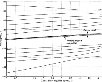
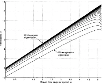
2.2 Full eigen-spectrum for lc

=

4 with

N =

5 33 2.3 Zoomed eigen-spectrum for rc

=

4 with N

=

50 34 2.4 Comparison of incompressible linearized and Rossby-Haurwitz solu-

tions for n = 3,4 and 5 with

N =

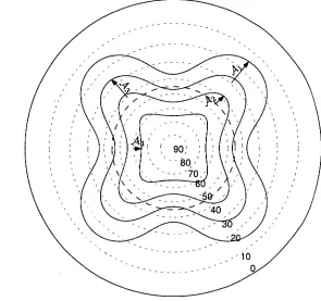
100. 36 2.5 Incompresible shallow atmosphere free-surface contours for it = 4

with

N =

100. 37

2.6 Rossby—Haurwitz free-surface contours for n = 4 37 2.7 Incompressible shallow atmosphere free-surface contours with corre-

sponding velocity vector field for lc

=

4 with

N =

100 38 3.1 Various amplitude measurement methods 56 3.2 Incompressible wavespeed versus amplitude for Ic

=

4 and w = 1.25 . 59 3.3 Incompressible shallow atmosphere free-surface contours for it

=

4,

c4.) = 1.25 at limit of computation. The average amplitude is Aave

12.5104(deg.) and the wavespeed is c= 0.9580 60 3.4 Incompressible wavespeed versus amplitude for it = 4 and w = 1.0 62 3.5 Incompressible shallow atmosphere free-surface contours at end of

branch 1 for it = 4, w = 1.0. The average amplitude is Aave

=

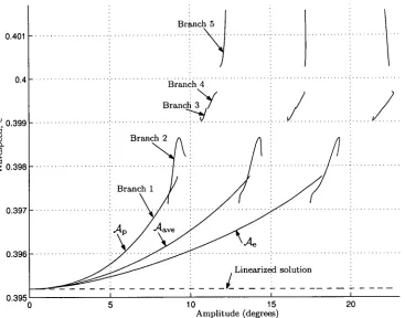
13.6732(deg.) and the wavespeed is c = 0.3978. 64

(13)

LIST OF FIGURES

vii

3.6 Incompressible shallow atmosphere free-surface contours at end of

branch 4 for tc = 4, w = 1.0. The average amplitude

is Aave

17.11662(deg.) and the wavespeed is c = 0.3997

65 3.7 Incompressible shallow atmosphere free-surface contours at end of

branch 5 for n = 4, w = 1.0. The average amplitude is

Aave

17.11662(deg.) and the wavespeed is

c =

0.4016.

66 3.8 Incompressible shallow atmosphere free-surface contours with

corre-sponding velocity vector field at end of branch 5 for

lc =

4, w = 1.0.

The average amplitude is ,Aave = 17.11662(deg.) and the wavespeed

is

c =

0.4016. 67

3.9 Incompressible wavespeed versus amplitude for n =- 5 and w = 1.25 68

3.10 Incompressible shallow atmosphere free-surface contours at end of

branch 1 for ic = 5, w = 1.25. The average amplitude is

—ave A

_—

8.3678(deg.) and the wavespeed is

c

= 1.5812

70 3.11 Incompressible wavespeed versus amplitude for n = 5 and w = 1.0. 71

3.12 Incompressible shallow atmosphere free-surface contours at end of

branch 1 for

ic =

5, w = -1.0. The average amplitude is

Aave =

9.3175(deg.) and the wavespeed is c = 0.9945

72 4.1 Free-surface height parameters

75 4.2 Comparison of compressible linearized and Rossby—Haurwitz solu-

tions for

ic =

3,4 and 5 with

N =

100

92 4.3 Compressible linearized free-surface contours for

lc =

4 with

N =

100. 93

4.4 Compressible linearized density contours for

IC =

4 with

N =

100. . . 94

4.5 Compressible linearized pressure contours for it = 4 with

N =

100. . 95

4.6 Compressible linearized pressure contours with corresponding veloc-

ity vector field for ic = 4 with

N =

100

95 5.1 Compressible wavespeed versus Amplitude for n = 4 and w = 1.25 . 104

5.2 Compressible free-surface contours at end of branch 2 for /c = 4,

(14)

5.3 LIST OF FIGURES

Compressible free-surface contours with velocity field at end of branch

viii

2 for n = 4, co = 1.25.

106 5.4 Compressible wavespeed versus amplitude for tz = 4 and co = 1.0 . . 107

5.5 Compressible wavespeed versus Amplitude for n = 5 and co = 1.25 . 108

5.6 Compressible wavespeed versus Amplitude for tc = 5 and co = 1.0 . . 110

C.1 Rossby-wave viewer output, Equatorial region

121 C.2 Rossby-wave viewer output, Antarctic polar region

122

(15)

CHAPTER 1 INTRODUCTIO

1.1 Brief Literature Review and Research Objective

Since the classic paper by Rossby [69], proving the existence of large-scale planetary waves in the atmosphere, there has been much interest and time devoted to un-derstanding and describing these planetary waves, known throughout the scientific community as Rossby waves. In particular, how Rossby waves influence the global circulation of the atmosphere has been the focus of a wide body of research over the past sixty years and it has been suggested by Lorenz [58], and later supported by Lilly [50], that the dynamical stability of Rossby waves might impose a limit on the overall numerical predictability of the global circulation.

Traditionally, almost all analytical and numerical analysis of planetary waves has been carried out either on a localized tangent plane to a sphere, the 0-plane, or else with a simplified set of governing equations for the full spherical geometry. The benefits of these two approaches are that the recovery of closed form wave solutions to the equations under consideration is often possible, of which the wave forms found by Rossby [69], Haurwitz [32] and Longuet-Higgins [54, 55] are classic examples. In this thesis, following work first introduced by Haurwitz [32], we make no tangent plane simplifications and we use the shallow atmosphere equations for a thin layer of fluid with a free-surface on a rotating sphere. The aim is to incorporate the exact spherical geometry in the governing dynamics.

The shallow atmosphere equations, or shallow water equations if dealing with ocean- ography, have been used extensively in dynamic meteorological modeling. The paper by Williamson et al. [87] has subsequently generated a large literature of research

(16)

1.1. BRIEF LITERATURE REVIEW AND RESEARCH OBJECTIVE 2

papers using the shallow atmosphere equations as a basic test bed for fast global atmospheric solver algorithms (see, e.g. [9], [17], [40], [79]). Their test case 6 em-ploys the Rossby-Haurwitz wave, with parameters similar to those first used by Phillips [66], to initialise the flow state which is subsequently computed at later time steps. While the Rossby-Haurwitz wave is useful here as a flow initialiser, it is important to remember that it is not an exact analytical solution of the full nonlinear shallow atmosphere equations.

Indeed, there is recent numerical evidence by Thuburn

&

Li [81] that the zonal wavenumber 4 Rossby-Haurwitz wave is dynamically unstable and will eventually break down as the result of an initial perturbation. This agrees in general with previous work conducted by Hoskins [39] and Baines [6] who both found maximum amplitudes beyond which instability of Rossby-Haurwitz waves subject to pertur-bations was observed. All these results serve to highlight the fact that Rossby-Haurwitz waves, while analytic solutions of the barotropic vorticity equation, are not true solutions of the shallow water equations on a sphere.

Another possible source of instability for Rossby waves could be the presence of nonlinear resonances, as certain key flow parameters are changed. Resonances are known in the water-wave literature, and are characterised by the presence of two or more solution branches in close proximity. Resonances in large-amplitude free-surface waves were apparently first encountered by Wilton [88], in the context of gravity-capillary waves. Schwartz

&

Vanden-Broeck [72] and Hogan [34, 35, 36] subsequently showed that the small divisors in Wilton's resonant solutions are indeed associated with multiple solution branches. Forbes [24, 25] encountered a similar phenomenon in waves beneath a floating elastic ice sheet.

(17)

1.1. BRIEF LITERATURE REVIEW AND RESEARCH OBJECTIVE 3

wave solutions of the shallow atmosphere equations, with different disjoint solution branches existing at different values of the forcing amplitude. Thus, small pertur-bations to a Rossby-Haurwitz wave which has been used to initialise a numerical solution of the shallow atmosphere equations, could cause the wave to fluctuate be-tween one solution branch and another in an unpredictable fashion, or break down structurally altogether.

The main goal of this thesis is to extend the above literature by finding numeri-cal solutions of the shallow water equations in the form of progressive Rossby waves that propagate in time without change of shape. Additionally, we aim to explore the relationship that exists between the nonlinear progressive wavespeed and wave am-plitude. Two distinct models of the atmosphere are investigated; an incompressible model is first considered and then, in the second half of the thesis, a compressible model is analyzed. The approach is mainly through numerical methods so it must be emphasized at the outset that the task of determining the nature of the exact physical processes that produce some of the subsequently observed results is some-what hard to discern; a separate analytical study, to which an entire thesis could be devoted, would be needed in many instances. Our aim, therefore, is to uncover key qualitative aspects of progressive Rossby wave solutions for the models under examination.

In Chapter 2 we derive the incompressible shallow atmosphere equations for free-surface fluid flow on a rotating sphere. After non-dimensionalizing, we construct a linearization by first finding a base westerly zonal flow and then perturbing about this state. Solutions are sought in the form of Fourier series with specific symmetry conditions and a standard Galerkin method is used to integrate the linearized equa-tions in closed form, leading to a generalised eigenvalue problem for the wavespeed which is readily solved. Comparison is made to the equivalent Rossby-Haurwitz solutions found in [32], with excellent agreement observed between the separate theories.

(18)

1.2. PRELIMINARIES 4

wave amplitude in terms of one of the unknown Fourier coefficients. A detailed pic-ture is developed of how the progressive wavespeed depends on the wave amplitude, revealing the presence of nonlinear resonances.

A compressible shallow atmosphere model is derived in Chapter 4. It is shown that if the values of the pressure and density on the free-surface are assumed to be zero, which is consistent with the concept of the atmosphere terminating there, then the model almost reduces to the incompressible dynamics, with the only difference being a slightly modified conservation of mass equation. Similar techniques to those used

in Chapter 2 are applied to the compressible equations, providing small amplitude _>-

linearized solutions of the model. CC

CC The solution of the full nonlinear dynamics of the compressible model is accom-

plished in Chapter 5. The linearized results of Chapter 4 are extended by comput-ing nonlinear solutions via a bootstrappcomput-ing process, providcomput-ing detailed information

on

how the nonlinear progressive wavespeed and amplitude are related. The effect of compressibility is observed to manifest itself via damped resonance behaviour in general.

Cr)

A brief discussion in Chapter 6 concludes the thesis. In closing, some conjectures are CC u_i made as to how the results obtained might help explain certain observed atmospheric

phenomena. In particular it is proposed that the process of atmospheric blocking is a direct result of critically forced stationary Rossby waves. If this conjecture is true, it would support the blocking theory of multiple equilibria that is popular amongst many theoretical meteorologists. Lastly, a visualisation tool that was developed to aid in interpreting the results, using the OpenGL three dimensional programming interface, is briefly documented in Appendix C.

1.2 Preliminaries

(19)

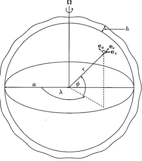
[image:19.569.187.417.339.600.2]

We consider a spherical model Earth of radius a and rotating with constant angular velocity

Cl,

enveloped by a model incompressible atmosphere, with a free-surface, of depth h(A, 0, t). A spherical polar coordinate system (r,

)., 0)

is defined, in which r measures the euclidean distance from the origin of the coordinate system and A is the azimuthal (longitudinal) angle coordinate. An elevation (latitudinal) coordinate

0

is also defined as the angle above the equator, so that the North and South poles are represented by

0 =

7/2 and

0 = —

7/2 respectively. This is not the standard definition of polar angle

0

common in most instances (see, e.g. Kreyszig [44, pages 498-499]), although it is usual practice in meteorology (e.g. Dutton [21], Haltiner

SL

Williams [31], Holton [37]). A schematic diagram illustrating the coordinate system and enveloping atmosphere is given in Figure 1.1.

Figure 1.1: Spherical coordinate system with free-surface.

(20)

In a reference frame rotating with angular velocity 11, conservation of mass for an inviscid fluid is expressed through the continuity equation

Dp

—Dt + PV = °

and conservation of momentum requires the usual Euler equation

Dq 1

—Dt + x q + -Vp = f, (1.2)

where f is the combined effect of all body forces per unit mass. The total (substan-tial) derivative in (1.1) and (1.2) is defined as

D 0

Dt =

at±q•v'

(1.3)

and the gradient and divergence operators appearing in (1.1), (1.2) and (1.3) are appropriately defined for the spherical polar coordinate system represented in Fig-ure 1.1.

Conservation of energy, in the absence of viscous dissipation and thermal conduction, is expressed through the first law of thermodynamics and is given mathematically as

DT pDp

Pcv Dt p Dt = Pqh. (1.4)

In (1.4), T is the temperature, ct, is the specific heat at constant volume, and qh is the rate of heat addition per unit mass by internal heat sources. This study will only be concerned with fluids that are either incompressible, so that the density p is constant, or compressible and ideal, so that the ideal gas law of the form

p = pRT (1.5)

can be used to approximate the thermodynamic state relations. The symbol R in (1.5) is the gas constant for dry air and will always take the value of

R = 287J kg' K' in this work.

(21)

1.2. PRELIMINARIES

7 Mass

Op Op u,, Op nOp

at

Or ± r cos 0 aA ± r 00

a a

P

[ a

(r

2 u, cos

0)

+ —

(ru

A

)

+

—

(ru

o

cos 0)] =

0, (1.6)

r

2 cos 0

ar a), ao

r momentum

aUr aUr U), aUr U4, aUr U 4- 2 U 2 1 Op

+ Ur - + A CA

2/2u

x

cos 0 +

= -g,

(1.7)

at Or r cos 0 OA r 00

p Or

A momentum

au„ au„ u, au, It

o

au„

+ Ur

Ot Or r cos 0 OA r

ao

uru, — u„u,

tan

0

1 Op

+

212 (u,. cos 4)

n

o

sin 0) +

= 0, (1.8)

r

pr cos 0

aA

4)

momentum

au

o

u„

_{+ au}

o

au

4 ,

+ u

r

—

at Or

r cos 0 OA r 00

u

r

u

o

+ u2, tan

0 1 al,

+

21 -

2u

A

sin

0 +

—

pr

—

a0

=

0, (1.9)

Energy

Pcv [—

OT

Gas Law

OT

u,

OT u

4 , aT1

Or r cos 0

a),

r

ao]

p [Op Op

u

A

Op

- - — + u — +

p at

r

Or

r cos 0 OA

+

—r —00

1 =

Pqh,

(

1 .

10 )

p = pRT.

(1.11)

Equations (1.6)-(1.11) form a closed set, for field variables Ur, u

A

,

p, p

and

T,

that model compressible ideal fluid flow in a rotating spherical reference frame.

(22)

CHAPTER 2 INCOMPRESSIBLE LINEARIZED

SHALLOW ATMOSPHERE MODEL

2.1 Derivation

[image:22.571.208.388.494.681.2]

We consider here the basic derivation of the incompressible shallow atmosphere equations following the general approach developed in Pedlosky[65, pages 57-63]. However, as opposed to the rotating cartesian form derived in [65],we initially start in a rotating spherical coordinate system, thus allowing for the curved geometry of the spherical Earth to be appropriately incorporated into the resulting equation set.

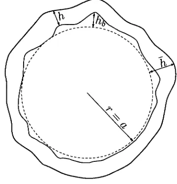
Figure 2.1: Free-surface height parameters

Commencing the derivation we define ft as the height of a free-surface surrounding a rotating reference sphere of radius r = a as depicted in Figure 2.1. We measure ii,

(23)

2.1. DERIVATION 9

as the radial distance from the level surface r = a of the spherical coordinate system to the free-surface. Additionally, define h and hb as the depth of the fluid and the height of the underlying mountains respectively. The height of the free-surface

h

can be given in terms of the two parameters h and hb as

h=hb+h. (2.1)

Although the generality of this setup affords the representation of a much wider class of problem we will restrict ourselves to the case when there is no underlying mountain specification so that hb = 0, leading to

h = h. (2.2)

Because we are only concerned with incompressible flow in Chapters 2 and 3, the equations of motion presented in Chapter 1 will reduce significantly. In particular, since density p is constant the mass equation, (1.1), reduces to the form V • q = 0. In addition, we can discard all thermodynamic behaviour, allowing us to remove the energy and ideal gas_equations from the governing system. We also note that, due to the nature of the spherical coordinate system, the vertical coordinate r appears explicitly in the dynamical equations. Holton • [37, page 24] points out that these curvature terms can be adequately approximated by r = a since the depth of the atmosphere h is assumed to be much smaller than the radius of the earth. Adopting the above approximations and simplifications we obtain the following form for the incompressible dynamical equations.

Mass

au, au, a

a cos 0-79-7--. + + (uo cos 0) = 0, (2.3) r momentum

au,

Our

u,

au, u

,,, Ou

r

tt2A + 1

ap

+ u — +

2ou„

cos

0 + —

p

—

ar

= —g, (2.4)

at r

Or

a cos cb

a A

a

ao

a A momentum

au„ au,

u„

au„

u

o

au,

+

+ r u —

u

r

u, —

uxuo tan 0

at

Or a cos

0

OA a a0 a

1 Op 2S-2(ur cos cb — uo sin 0) +

(24)

2.1. DERIVATION

10 (/) momentum

Ouct,

au

o

u

A

au

o

no Ono

u

r

u

o

+

u2),

tan

0

+ u

r

— +

at ar a cos 0 aA a 00 a

+ 2Qu

A

sin 0 + —

_{ap 00}

1 p

0. (2.6)

The underlying assumption of the shallow atmosphere approximation is that motion

mainly occurs in the A-0 plane and less so in the r direction, effectively confining

the velocity to predominantly "horizontal" motion. Mathematically we can write

this statement as

Ur

u

x

0(c),

0(1),

(2.7)

(2.8)

0(1),

(2.9)

where

E

is a small parameter that reflects the shallowness of the atmosphere relative

to the radius of the Earth. In effect,

E

might be regarded as the ratio

h I a

which

is typically of order 10

-3

for the Earth. Consider now the implications of this

ap-proximation for the r momentum equation (2.4). We argue that the total derivative

ternasu

_{at , r}

_a

_acosck

aur and —

_aA

_a

a

_ao

ur are all

0(c)

so that the r momentum equation

reduces to

U2 ± u2

ap

(2.10)

A

a

ck 25-2uA cos

0 +

-

p

-

—

ar

=

-

g,

where only terms of 0(1) have been retained. Finally, we assume that (2.10) is

dominated by hydrostatics', so that effectively we have

ap

=

-pg.

(2.11)

Equation (2.11) can be integrated with respect to r, yielding

p(r,

A,

0,

t) =

-

pgr + f (A, , t).

(2.12)

We fix the value of

f

(A,

0, t)

by assuming that, on the free-surface r = a + h(A, 0,

t),

the pressure has the constant value P

o

so that

P(r,

A, 0, t) = Po

pg(a +

h(A, , t)

-

r).

(2.13)

(25)

2.1. DERIVATION 11

From (2.13) we immediately obtain

OpOh

_

OA – Pg OA'

Op

_

ah

—

Pg-

a

--

;

(2.14) (2.15) implying that the horizontal pressure gradient components are independent of r, which in turn implies that the horizontal accelerations must be r-independent also. It is therefore consistent (see Pedlosky [65, page 61]) to assume that the horizontal velocity components are also r-independent if they are initially so. Thus we must have

(2.16) (2.17) so that, in conjunction with (2.7), the two remaining momentum equations, (2.5) and (2.6), taken to 0(1) become

A

momentum

aux ux

au

x

uo aux uAuo tan 0 g

Oh

+

2/2/4

1, sin 0 + = 0, (2.18)

at

+

a cos c

h DA

a 00 a

ap cos 0 OA

(/) momentum

aucto uA

au

g

,

uo

au

o

u2„, tan 0

g Oh

0t + a cos 0

aA +

a

00

+ a + 2QuA sin 0 + —

ap

—

00 = O.

(2.19) We now turn our attention to the mass equation and note that since u A and u4, are r-independent we can integrate (2.3) with respect to r to give

OuA a

a cos 0

u

r

(r, A, 0,

t)

= –r [–a-5-k- + (no cos 0)] +

it,

(A, 0,

t).

(2.20) To determine the nature of ft, we need to examine the boundary conditions on the upper and lower boundaries r = a +

h

and r = a +

hb

respectively. On the lower boundary we must have no normal flow, otherwise the fluid would penetrate the surface and breach the conservation of mass requirement. Thus on r = a +

hb

we must enforce the condition q • n = 0 where n is a normal to the surface r = a +

hb.

We can easily show that the normal to the lower boundary is given by 1

_{ahb 1 ahb}

n = er a cos eA – 4,

(26)

2.1. DERIVATION 12

so that

q • n = ur(a hb, A, 0, t)

Solving for 'Ur we obtain

UA ahb uhb 0

a cos 0 aA a

80

—

(2.22)

u), ahb u4, ahb ur (a + hb, A, 0, t) =

• (2.23)

a cos

0 DA

± —

a

a0

Substituting (2.23) into (2.20) and evaluating at r = a ±

li

b

allows us to solve for

fir, which we in turn substitute back into (2.20). After simplification we arrive at

au„ , , a

a cos 0 ur (r, A, 0, t) = -r [79-A- 014, cos 0)1 (uxhb)

a

+ — (u

_a

o

h

b

cos 0) .

(2.24) On the upper boundary we enforce the kinematic condition

Dt [r - a - h(A ' t)] =

which states that the fluid can not penetrate the free-surface. Expanding the total derivative and solving for it,. gives

ur(h, 0,t) = —ah

_{at +}

u, ah ucs ah

(2.25) a cos

aA

4-

a

ao

.

Finally, substitution of (2.25) into (2.24) and subsequent simplification yields the incompressible shallow atmosphere mass equation given by

ah a

acos + 0

,u,(h — hb)) + —

_

_{a (uo(h}

_a

_—

_-

— hb) cos 0) =

0.

at

a

A (2.26)

We note that since h = Ii - hb, expanding all differential products and writing

f =

2l sin 0, we can express the complete dimensional dynamical equations of motion for an incompressible fluid in a rotating spherical coordinate system as mass

ah ah

It

o

a

h

[„u

a

)

, au

o

+ a cos ± ± a cos

+ cos 0 - u

o sin 01 = 0, (2.27)

at 0 aA

a 00 0

DA ao

A momentum

au„ uA

au

A

u

4 , (9u),

_g

ah

=

0, (2.28)

at

+

a cos

°A

a

ao

a a cos 0

aA

momentum

au,,

UA aU4,

auo

_g

ah

0.

(2.29) (k (f

+

tan 0) u +

(27)

2.2. PROGRESSIVE-WAVE COORDINATE TRANSFORM 13

The above form is that given by Williamson et al.[87, page 213] as the advective form of the shallow atmosphere equations and this is the form we shall subsequently use for all analysis in this chapter.

2.2 Progressive-Wave Coordinate Transform

We are interested in solutions to equations (2.27), (2.28) and (2.29) that are of the form of a progressive-wave with constant angular velocity. Defining c to be an angular wavespeed we now construct a new moving coordinate frame that depends on A and

t

in the form

n

=

A – ct. (2.30)

The effect of the

–ct

term is to translate any initial wave structure either towards the west

(c <

0) or towards the east

(c >

0) with constant angular speed

c.

Since we have defined a new coordinate system we need to establish how the equations of motion are represented in this new reference frame. Applying the chain rule we can easily show that, for some scalar field tIf

(77,0),

ow —

ow

--= ,

A

0,\.

a n

(2.31)

ow &Ta

_{= -- =}

n

ow

–c

. (2.32)

at ail at ar,

Using this transformation we can now write equations (2.27), (2.28) and (2.29) as mass

(u,

Oh

u cos

an

0

— – c cos ck) 4, h

[

a

11,, Ouo

+ – — + cos 0 – uo

sin

a

an

a a

ao n ao

d = 0,

A momentum

(2.33)

(

u), , au,

u4, cos 0

au,

(

f cos 0 +

sin

0)

uo

–

g

—

Oh

=

0, (2.34)

— – c cos

a a

ao

a an

(j) momentum

(

u, auo uo cos

0 +

(f cos 0 +

ui

sin 0) uA

g cos q5

an

— — ccos o

_a

=

0, (2.35)

a

ao

a a

Do

(28)

2.3. NON-DIMENSIONALIZATION OF THE GOVERNING EQUATIONS 14

2.3 Non-dimensionalization of the Governing

Equations

In an attempt to generalise the analysis, it is desirable to express the governing

partial differential equations in a form that is independent of the specific units used

to measure the variables of the problem. For this reason we non-dimensionalize

each of the governing equations to expose the underlying qualitative behaviour.

The particular approach adopted here is similar to that used by Klein [42, page 766]

in that we reduce our dimensionless parameters to the set of familiar fluid dynamical

parameters comprised of Strouhal number, Froude number and Rossby number.

First we define the following characteristic values, for each reference scale contained

in the problem, as

v„

f

characteristic speed,

h

ref

characteristic free-surface height,

c„

f

characteristic angular velocity.

Using these dimensional parameters we now rescale all the field variables to

dimen-sionless form giving

fLA = - = VUrief

UA 7-4°114'

Ito

114, = UA = Vreffickl

v rrr cee f

= h

h =

hrefirt,

h

f

C

ef

(2.36)

(2.37)

(2.38)

(2.39)

where the hat 0 denotes a dimensionless variable. Substituting equations (2.36)–

(2.39) into (2.33), (2.34), (2.35) and manipulating, we obtain

mass

c„

f

a

all ail a

it

o

u

0 — +n

c cos

o

cos 0— +h — +

cos 0

—

/1

4

,

sin

0 = 0, (2.40)

v

ref

jar1

ao

A

momentum

(fi

x

c

ref

a , 0 , ft ),

c

cos

op)

— + u

4

,

cos 0 (

— cos 0 +

2C2a

fix) '

ri

ck

sin

v

ref

0

77

0 0 v

ref

gh

ref

h

+2 0,

(2.41)

(29)

2.4. LINEARIZATION OF THE EQUATIONS 15

4) momentum

Crof

a

C

cos

0)

— + ito cos (P +

a u a u

_{an a}

o

2S2a

—

cos 0 + ft sin

o

(15

//ref

o

gh

rof

cos

0 a h

v,?„

a

o

=

0 '

(2.42)

where we have also replaced the Coriolis parameter

f

by its definition

f =

21/ sin 0.

Three obvious dimensionless parameter groupings emerge from this process. These

are just the familiar flow regime parameters from fluid dynamics given as

a

Crcf

Sr = Strouhal number,

v

ref

Vrcf

Fr =

Froude number,

VF1

-

t7

c

;

v

ref

Ro = Rossby number.

_2S

.

2a

Substitution of these parameters into our governing equations yields

mass

[a ?I

A

(fi

x

— Sr c cos) — + u

0 o

cos 0

—

+

h +

cos

cb

a 114

) - ^ •

an a o

-

a

-

7 1 a

u

o

sm =0, (2.43)

A momentum

aU

A

, au

x

cos

cb

1 alt

(u

A

-

Sr a cos 0) a

+ "

ct

, cos o

p

—

-

an ao (

6

—

R7

3. -"A

-

) 116 sin

ck

0, (2.44)

4, momentum

au au

(u

A

-

Sr

cos 0) +

cos +

_ao

(cos 0

+)

it

,

sin

, cos

0 =

0, (2.45)

Ro su "

1-

Fr

2 which is the final form for the non-dimensional incompressible shallow atmosphere

equations on a rotating sphere.

2.4 Linearization of the Equations

2.4.1 Base Zonal Flow Derivation

As previously discussed in Chapter 1 it is convenient to consider Rossby waves as

consisting of latitudinal perturbations about an underlying zonal flow structure.

Thus it is important to know the exact nature of the zonal flow in order to calculate

(14

(30)

2.4. LINEARIZATION OF THE EQUATIONS 16

the resulting perturbations. Following the work of Haurwitz[32, page 255] we choose the simplest zonal flow in the form of a super rotation that only depends on latitude and additionally has u4, = O. The form for our zonal flow is then given by

zt,„ = w cos 0, (2.46)

uo, = 0, (2.47)

hz = (2.48)

where the parameter w is the non-dimensional representation of the base angular speed of the flow and the subscript

z is used to denote field variables belonging to

the zonal flow structure. The problem now reduces to finding the function

H(0)

that makes equations (2.46), (2.47) and (2.48) a solution of equations (2.43), (2.44) and (2.45).

Direct substitution reveals that the only equation not identically satisfied by the zonal flow structure is the 0 momentum equation, which yields the ordinary differ-ential equation

dH

= —wFr 2 ( -1 + CV )

c

sin 0 os 0.

d0 Ro

This integrates easily to give

wFr2 1 H(0) = ho +

2 (Ro + w) cos20.

(2.49)

(2.50)

The constant of integration h, can be viewed as the base non-dimensional height of the free-surface at the poles and typically we would choose h, = 1 so that the dimensional value of hz at 0 = +7/2 is href . The two parameters w and h, suffice to specify uniquely any given super rotation and associated total mass, or volume in the incompressible case, of the system. We note here that in order to make comparison between results with differing values of w it is necessary to modify the value of h, so that the total volume of fluid in a +

hb

<r <a + h remains constant. This amounts to solving a cubic equation for 110 once a fixed volume and value for w have been decided upon.

(31)

In summary, we have shown that a basic zonal flow structure is given by

ILA z

=

(i) cos 0,

uoz = 0,

wFr2

h

z

=

+

(2.51) (2.52) (2.53) 2 Ro

2.4.2 Linearization about the Base Zonal Flow

Given the base zonal flow we now consider 0(c) perturbations about this flow state by constructing the perturbation expansions

ux

(k)

₌

nAz+

EU„ (71, 0) 4- 0(E2 ), (2.54) U0(7

/7

q5)

=

0

+

EUoi (71,

+

O(e2),

h(n, 0)

=

hz

+

Eh

i

(n,q5)

+

0(c2).

(2.55)

(2.56) The perturbation parameter E is a small quantity that represents the maximum deviation about the zonal flow. It is instructive to think of c as a wave amplitude in this case, although it must be emphasized that the linearization is only valid for infinitely small amplitude and consequently our results will only be accurate as

—> 0. Nonetheless we can expect reasonable results for small values of E.

Substituting the perturbation expansions (2.54)-(2.56) into the governing equations (2.43)-(2.45) leads to the set of partial differential equations given by

mass

Oh

l

(u

Az

- Sr c cos 0) + euoi co

d

as:Id hz

au

/

Ehz + COS Ic9 Uoi sin d + 0(e2) = 0, (2.57) A momentum

,

d

uAz

(

cos cb

E (11 A z — Sr C COS lp ) — ElLoi COS 19 E —

d

IL A z ) Uoi Sill (1)

ari

ick Ro

1 ail,

+

(2.58)

cP momentum

( cos 0 cos 0 d h

z

alt

o

+ u

Az

u

A z sin 0 + ,, + E (2/Az — Sr c cos 0)

Ro Frz

d 0

Dr)

(cos

cos

0 oh,

+c cb + 220, z ) um sin 0 + 2 +

0(6

2 ) = 0. (2.59)

(32)

The 0(1) terms in (2.59) are satisfied identically by the base zonal flow. By putting uAz = w cos

0

into the above equations we obtain the 0(€) equations that define the first level of corrections in our perturbation expansions. These equations are mass

ah

i

d h

z

[au m tt

a

oi

(w -

Sr

c)

cos— 0 +

u

o

,

cos ¢, +

h — +

cos 0

u

o

,

sin

0]

= 0, (2.60)

an

_{d 0 an 00}

A momentum

aum

Go —

Sr

c) cos0—

(FL + 2w) uo, sin

0

cos 0 + — 1 ah, = ,,

an Fr2 an

u,

(2.61)

ck

momentum

cos

0 ah, _„

(co —

Sr

c)

cos

o'L

.--L

a + +2w)

ux , sin 0 cos 0 +

an

(ITO F 2

a

c

k

— u. (2.62) The solution of (2.60), (2.61) and (2.62) is facilitated by noting that we may write each of the

0(c)

perturbation terms as the product of a Fourier mode in n with a function of

0.

Thus we define

741(i7,

0)

=

cos(nn) A(0),

(2.63)

u(n, 0)

=

sin(kn)

st,

(q5),

(2.64)

=

cos(kn) H(0), (2.65)

where the parity of the Fourier basis in

ri

in each term is chosen to preserve the overall parity of each dynamical equation. Alternatively, it would be possible to interchange the sin and cos terms in (2.63)-(2.65), with the effect of rotating the solution at

t=

0 by

71K.

Also note that the parameter n has been introduced as a way of specifying the wavenumber of the solution. This is a natural addition to the model since intuitively we would expect that the wavespeed c will depend on the number of equally spaced wavelengths around a latitude circle.

By defining our

0(c)

terms according to (2.63)-(2.65) we can remove the n depen-dence entirely from the partial differential equations, transforming them into a set of ordinary differential and algebraic equations given by

mass

d h

z

k (w -

Sr c) cos 0 H(0) + (I)(0) cos 0 d 0

d(0)

+

hz

[-kA(0) + cos

0

413 (1.

(33)

2.5. NUMERICAL SOLUTION OF THE LINEARIZED EQUATIONS 19

A momentum

1

—tc(w — Sr c)

cos0

A(0) — (—

Ro + 2w) (I)(0) sin 0 cos 0 — Fr2 = 0, (2.67) 0 momentum

1

((V - Sr

_c)

4)(0) + (11 ±

2w) A(°) sin (k Fr2

d

1

d )

= °.

(2.68)

2.5 Numerical Solution of the Linearized Equations

2.5.1 Series Representation

The numerical solution of (2.66), (2.67) and (2.68) can be accomplished by approx-imating each of A(0), (DM and

7 -

00)

with truncated series of basis functions. As noted by Boyd[10, page 109], the particular choice of basis function is primarily governed by the geometry involved in the problem. The inherent spherical geome-try in the shallow atmosphere problem can be adequately described by using either spherical harmonics or Fourier basis functions, which both cope well with periodic boundary conditions. Although the generally accepted solution approach for prob-lems in spherical geometry, in both meteorological and mathematical circles, is via the spherical harmonics, the sheer simplicity and ease of use of Fourier series is an attractive alternative that, as will be demonstrated shortly, allows for some further analytical manipulation to be carried out, greatly reducing the computational time for any given solution.

The particular form of the Fourier basis components needs careful consideration, primarily because we can identify key symmetry and boundary conditions that each of the field variables must satisfy. In this study we are only concerned with special types of solutions that obey the following set of conditions:

• u), and

h

are symmetric with respect to the equator (0 = 0), • uo is anti-symmetric with respect to the equator,

• u), and u,,, are zero at the poles (0 = ±7/2),

• h

is constant at the poles.

(34)

that a northward velocity deflection in the northern hemisphere is equivalent to a southward velocity deflection in the southern hemisphere, whereas the free-surface has the same height at points (no, ±00). From the above list of solution requirements we can also deduce that the 0(i) field variables must all have zero value at the poles. This is necessary because we have convergence of lines of longitude at 0 = ±7/2 and hence to avoid multi-valued functions for the field variables we require that the perturbations are all zero at the polesiii .

Although the above list of solution requirements might seem, at first glance, to be rather restrictive there is much to be gained by employing such an approach. The main advantage of this formulation is that difficulties at the poles are avoided; this can be a common source of numerical trouble in models that account for the spherical geometry. The pole problem amounts to the previously mentioned dilemma of having multi-valued functions defining the flow field and the apparent switching of East to West (or North to South) as one traverses across a pole of the spherical coordinate system. A common approach to navigate this troublesome numerical stumbling block is to introduce new velocity components that are multiplied by Fourier functions that correctly adjust for the parity change on either side of the pole as detailed in Duran[20, page 207]. In our approach no such adjustments are required since by forcing the flow to have stagnation points at each pole we will never encounter a scenario in which flow with an eastward or northward component suddenly switches to flow having a westward or southward component. Of course, in all realistic global circulation models the handling of the pole problem becomes an integral feature of any time integrating computation since in general stagnation points are not situated at both poles. Nonetheless, the advantages to be had by adopting our approach coupled with the motive of theoretical investigation justify its use.

We are now in a position to construct the series approximations. For now we just state the forms for the 0(i) linear terms, defering the statement of the series for the full nonlinear terms until Chapter 3 when we approach the solution of the full nonlinear system. The functions that meet our prescribed conditions above can be

(35)

given by

A(o)

_=>2

Pk

,flcos((2n— 1)0), (2.69)

n=i co

c

o

) E

Q sin(2n0), (2.70)

n=i co

7-00)

E

H,,,n (-1)n [cos(2n0) + cos(2(n — 1)0)] , (2.71)

n=1

where subscript n on each coefficient denotes the longitudinal wave number that we are currently using as defined in equations (2.63)—(2.65).

It is also essential to point out that the particular form of (2.71) is due to the process of basis recombination in which we have constructed new basis functions, which are linear combinations of our underlying basis set, that satisfy the required boundary conditions, as discussed in detail in Boyd[10, page 112]. Basis recombination is needed here since the general representation of h(n, 0) need only be constant at the

poles, rather than zero as in the case of the two velocity components u,, and uo.

Thus the underlying basis set is centered around cos(2n0) which attains the value of ±1 at the poles. Since we require 7-1(0) to be zero at ±r/2 then it becomes the task

of basis recombination to satisfy this boundary condition; this is achieved through the particular form of (2.71).

2.5.2 Galerkin Method

With the forms for each of our series defined we now tackle the problem of solving for the wavespeed c and associated coefficients - kP m, Q and 11,,n. To do this we

exploit the orthogonality properties of the trigonometric functions by requiring that the residual equations, obtained after substituting (2.69)—(2.71) into (2.66)—(2.68), be orthogonal to each of our expansion functions. This technique amounts to the standard Galerkin method which has been used extensively to solve optimization and root finding problems from all areas of mathematics. We now demonstrate the particular application to our problem.

(36)

mass equation given by

–tc(co – Sr

c) H,,n (

–1)n [cos(2m) cos ç5 + cos (2(n – 1)0) cos 0] n=1

oo — WFT*2 (—

Ro + co)

E

sin(2n) cos 2

0

sin 0

n=1

oo coFr2 ( 1

± +

_{2 Ro}+ co) cos20) [–k

E

Pis,n COS((2n 1)0)

n=1

0.

00 + E c2„,n2n

cos (27/0) cos –

E

Q ,,n

sin(2n0) sin 01 = 0. (2.72)

n=1 n=1

We can show that general terms of (2.72) take the form cos((21 – 1)0), for / I, 2, ..., so these become our base expansion functions and the orthogonality con-dition is now equivalent to multiplying (2.72) by cos((21 – 1)0), integrating from –7r/2 < < 7r/2 and equating to zero. Performing these operations we have

00

–n(co – Sr

c)

E

I

72'

cos(2n0) cos 0 cos ((2/ – 1)0)

c/0

n=1 oo

IC(W — Sr.c)

E

cos(2(n – 1)0) cos 0 cos ((2/ – 1)0)

d0

n=1

– coFr2 + co) °E) Q,,,n sin(2n0) cos20 sin 0 cos ((2/ – 1)0)

c/0

Ro _n=1

_ h

o

kE

P

K,n

cos ((2n – 1)0) cos ((2/ – 1))

c/0

n=1

oo

\

2

+

2h

0 ,,n cos(2n0) cos 0 cos ((2/ – 1)0)

d0

n=1

0 0

— ho

Q,,n

I

sin(2n0) sin 0 cos ((2/ – 1)0)

c/0

n=1

ru

,,

Fr

2 0.

2 Ro

+ w) E

P,,,n

I

cos ((2n – 1)0) cos20 coS ((2/ – 1)0)

c/0

n=1 oo

+ wFr2 (-1 + co)

E

nQ ,c,n cos(2n0) cos30 cos ((2/ – 1)0)

d0

Ro

n=1

WFr2

(37)

As an example, we consider the first integral in (2.73) and note that the integrand may be written, with the aid of the identity cos(A -B)+cos(A+B) = 2 cos A cos B , as

1

cos(2n0) cos 0 cos ((2/ - 1)0) = [cos ((2n + 1)0) + cos ( (2n - 1)0)] cos ((2/ - 1)0) 1

cos((2n + 1)0) cos((21 - 1)0) 1

+

-2 cos((2n - 1)0) cos((21 - 1)0). (2.74) In addition we then, if required, shift the index on the resulting integrands so that every integral in equation (2.73) is transformed to one of the form

/0 =

f

cos((2n - 1)0) cos((21 - 1)0)

do,

(2.75)

2 if n = /, (n 0 and / = 1) or (n = 1 and / = 0),

(2.76) 0 otherwise,

where the

o

subscript denotes an integral obtained by using orthogonality.

Applying trigonometric identities, similar to that used in (2.74), to all the integrals in (2.73) and then shifting the indices on those terms that require it we obtain

00 00

-(w - Sr

c)

E H,,,o

₊

,(-1)n+1/0 —

K(u) - Sr

c)

n=0 n=1

co wFr2 w\

— — (CV — Sr C)

Elkn—i(-1)n-1/0

+

8 Ro ) 2

n=2

[ co

E

QK

'

n-1-1-ro n=0

+

E

Q K,nio —

E

Q k,n—lio —

E

Q ic,n—go

I

— hoiC

E

Pn,nio

n=1 n=2 n=3

j

n=1

co oo

, ho co , ho °° + ho

E nqc,../-0 +

ho

E

(n - ini,n—lio — tc,nlo + —

2

E

QK,n—l-to

n=1 n=2 n=1 n=2

oo

kwFr2 /1 \ oo co

8

ii- ; + w) [E

o PK,n+li + 2 Ptc,n-ro +

E

Ptc,n-14

n=0 n=1 n=2

co

R2 ₁ oo oo oo oo

16

( Ro +w )

E Qr

_o

+ E

_{Q tc,n.ro}—

E

Q K,n—lIo —

E

C2k,n-2 10

n=

L

o n=1 n=2 n=3

wFr2 ( 1 w 00 + 00

8

+ ) [E(n + 1)(2K,n+11-0 + 3

E

nQ/o

Ro _n=0

n=1

+ 3(n - 1)qc,n-1-ro + (n - 2)Qn,n-2/0] = 0.

n=2 n=3

(2.77)

(38)

± [110

[ 2

3K,Lo

3/cwFr2 1 Kx.Rr 2 1 PK,/

+ w)] 8 8 ( Ro

wFr2 ( 1 wR2 ( Ro

1

icSr

--H

k

,2 + 8 3,c) w)]

n , 1 —

(±) Hk

2

=

C

± 16 3/cSr rj.

[

—

-- rc

2 Jan 1 -

w) Pit'2

1 (2.78) 2.5. NUMERICAL SOLUTION OF THE LINEARIZED EQUATIONS 24

Each integral

l

o

in (2.77) is now in the standard form given by (2.75) allowing us to use the orthogonality conditions given in (2.76) to extract a set of algebraic equations for each value of the integer

1.

Letting 1 = 1 and performing some algebraic manipulations we arrive at

where we have taken the terms involving the wavespeed c to the right hand side in preparation for the numerical solution method, to be discussed shortly. We also note that letting

1 = 1

is equivalent to letting

1 =

0 since the nature of the orthogonality of cos ((2n - 1)0) cos ((2/ - 1)0) is the same in both cases.

In a similar vein we now consider the case when

1 =

2, leading to ts,wFr2 /1 + w) + [ pk,1

+

rcwFr2 ( 1

Kho + w)] pk,2 ) co)] Qfro + w) Qtz73 8 Ro )

ni.,;Fr2 ( 1

Pk

4 Ro 3h 9wFr2 (±

[ 2

°

+

16 Ro +

±

8 Ro + w) '3

[3h0 9wFr2 1 3wFr2 1 [ 2 ± 16

(

Ro + w)] Qk72 + 16 Ro (

tiw_ H k 2 ± _KA.4.) ri ... _ [nSr , K2Sr

+ lik,3]

2 k1

+ KwH

' 7 2 rik73 - (-; 2 llto - icSrlik,2 + — (2.79) Finally, the cases for

1 >

3 are given by

IctoFr2 ( 1 + w) ,.,,, [ , nu.;Fr2 ( 1 + )1 T., 8 Ro r ,i_i + Kilo 4 Ro w r-K71

nc.oFr2

( 1

8 Ro Lo) PK7/-Fi + w(21 -

1)Fr2

( + w 1 +

16 —Ro ) Q tc,1-2

+ [(21 — 1)110

± 3(21 - 1)wFr2

( 1

2 16 Ro + w)] Qn 7/-1 [

(21

-2 1)1/0 +

3(21 -

1)wFr2 ( 1 + w)] c20

16 Ro )

w(21 - 1)Fr2

( 1

16 Ro + co) Qi

+ nti.,(-1)/

+ _ica-p

2 H,,,i _ i -

nSr(-1)/ icSr(-1)/

+

2 H„,1± 1 = c [ 2

H,

,1 1

IcSr (

-

1)1 Ho

2

(39)

Equations (2.78), (2.79) and (2.80) constitute an infinite set of algebraic relation-ships representing mass conservation that must be satisfied for a solution to be valid. In a similar manner we can derive equivalent algebraic relationships from both the A and 0 momentum equations, (2.67) and (2.68), by substituting our series expres-sions for the OW field variables and using orthogonality to generate the required equations.

From the A momentum equation we have: For 1 = 0, „ 1

— —I-pc ( 1 4.0) ts, - - r icSr 1 C[-

2 '1 — Q1 -

4 Ro Fr2 '

for 1 =1,

(2.81)

tc,CO IcCIJ 1 ( 1 ic 7.T

- r-tc 1 — w Q tc tc,2

2 ' 2 4 Ro Fr

=

c [

icSr nSr

- PK - _{2 2'}Pic 2 (2.82)

and for 1> 2,

tet,W K,CV 1 1 (1 (1

-2 Pk,/ - —2 Ptc'1+1 +

-4

—_Ro+w _{- -4} —_{Ro + w Qn,c+i} k(-1)/ 7., n(-1)1 , icSr nSr

K,

H _r2_{1+1 =}_—

2 1- ic'I 2 rtcp-i]

Fr2 F

Similarly from the 0 momentum equation we have, for 1> 1, 1 ( 1 u) .13K 1 ( 1 ±

2 1,o ) '1 2 Uto w ichoWtc,1

21(-

Fr2 tc, 1)1+1

±

H

24-1)1+1

2 HK,1+1 = C EKSrQn,/1 • Fr

(2.83)

(2.84)

2.5.3 Truncation and Generalised Eigenvalue Formulation

(40)

+ W) Pic,N-1 + [_

h

0

-1- w(2N -

1)Fr2

( 1

16 Ro +

w)

Qn,N-2 hu.oFr2 ( 1

8 kRo

Fr2 1 (

Our choice of equations from the set (2.78)-(2.84) is rather intuitive and obvious in that we use exactly N equations from each physical law. To elucidate this process we note that the orthogonalised version of the mass equation consists of two base equations, (2.78) and (2.79), and an infinite series of equations in the form of a recurrence relation (2.80). To obtain exactly N equations from this set we retain the first two equations along with N-2 from the recurrence relation so that the limit on 1 in (2.80) is now 1 = 3, 4, 5, ... , N. Note that when 1 = N we make reference to the coefficients _{P,,,N+1) QK,N+1}and

Ilk

,N+1 but these and higher-order coefficients are ignored in the truncation of the series (2.69)-(2.71). Thus when 1 = N we have the modified version of (2.80) given by

-F [

(2N -

₂ 1)110 3(2N - -E

1)wFr2

( 1

16 Ro 4- (4)1 C2N'iv-1 - 1)1z0 3(2N - 1)(h)Fr2 ( 1

2 -F 16 Ro + w)] Qic,N

±

21)N

II

k,N-1 — liAl(-

1)

N

II tc

,N

pcSr(-1) N

[ 2

H

tc

,N_i

—

nSr(-1)NHK,N]

=c

(2.85)

In a similar way we note that the orthogonalised version of the A momentum equa-tion also consists of two base equaequa-tions, (2.81) and (2.82), and an infinite recurrence set (2.83). Again, to obtain exactly N equations from this set we retain the first two equations and N - 2 equations from the recurrence relation so that the limit on 1 in (2.83) is 1 = 2, 3, 4, ... , N - 1. Since the maximum coefficient index is N, occuring when 1 = N - 1, we only index into coefficients that are members of the truncated set so no special treatment, analogous to that used to obtain (2.85) above, is required in this case.

(41)

2.6. SOLUTION AND RESULTS 27

this case. The result is

2 RO Pic'N trA-4)C2N'N

1 ( 1 2N (-1)N+1

Fr2 Hic,N = C[ICSrQ,,N]. (2.86)

The set of equations (2.78)-(2.84), coupled with the two special terminating condi-tions (2.85) and (2.86), constitute a complete generalised eigenvalue problem of the form

Ax = cBx,

where A and B are matrices corresponding to the left and right hand sides of each of our algebraic equations. The eigenvalue c is precisely the wavespeed for our progressive Rossby waves, and vector x is the eigenvector of unknown linearized coefficients which we define as

x =

I

HK,1\

tc,N

PIO

Prc,N C tc,1

(2.87)

\C2K,N/

We note that the general structure of both A and B is that of a banded diagonal matrix with A also containing banded sub and super diagonal components . In particular we note that diagonal matrix B consists of non-zero elements along the main diagonal and thus will be invertible, implying that we will always be able to find solutions of our generalised eigensystem.

Linear and nonlinear progressive Rossby waves on a rotating sphere