Aerodynamic design optimization using flow feature parameterization

Full text

(1)University of Southampton Research Repository ePrints Soton. Copyright © and Moral Rights for this thesis are retained by the author and/or other copyright owners. A copy can be downloaded for personal non-commercial research or study, without prior permission or charge. This thesis cannot be reproduced or quoted extensively from without first obtaining permission in writing from the copyright holder/s. The content must not be changed in any way or sold commercially in any format or medium without the formal permission of the copyright holders.. When referring to this work, full bibliographic details including the author, title, awarding institution and date of the thesis must be given e.g. AUTHOR (year of submission) "Full thesis title", University of Southampton, name of the University School or Department, PhD Thesis, pagination. http://eprints.soton.ac.uk.

(2) University of Southampton Faculty of Engineering, Science and Mathematics School of Engineering Sciences. Aerodynamic Design Optimization Using Flow Feature Parameterization. by Thomas Robin Barrett. Thesis for the degree of Doctor of Philosophy. November, 2007.

(3) UNIVERSITY OF SOUTHAMPTON ABSTRACT FACULTY OF ENGINEERING, SCIENCE and MATHEMATICS SCHOOL OF ENGINEERING SCIENCES Doctor of Philosophy. AERODYNAMIC DESIGN OPTIMIZATION USING FLOW FEATURE PARAMETERIZATION By Thomas Robin Barrett. Design optimization methods using high-fidelity computational fluid dynamics simulations are becoming increasingly popular in the area of aerodynamic design, sustaining the desire to make these methods more computationally efficient. Such design strategies typically define the aerodynamic product using a parametric model of the geometry, but this can often require a large number of design variables, increasing the computational cost. This thesis proposes that a parametric model of aerodynamic flow features, rather than geometry, can be a parsimonious method of representing designs, giving a reduction in the number of design parameters required for optimization. The parameterization of flow features is coupled with inverse design, in order to recover the corresponding geometry. While an expensive analysis code is used in evaluating design performance, computational cost is reduced by using a low-fidelity code in the inverse design process. This newly presented method is demonstrated using four case studies in 2-D airfoil design, in which the parameterized flow feature is the surface pressure distribution, and two case studies for 3-D wing design, in which the spanwise loading distribution is parameterized. These strategies are consistently compared against a benchmark design search method which uses a conventional parameterization of the geometry. The two methods are described in detail, and their relative performance is analysed and discussed. The newly presented method is found to converge towards the optimum design significantly more quickly than the benchmark method, providing designs with greater performance for a given computational expense. A parameterization of flow features can generate designs with higher quality and detail than a geometry-based method of the same dimensionality.. ii.

(4) Table of Contents Acknowledgments Nomenclature. xii xiv. Chapter 1. Introduction ................................................................................................. 1 1.1 1.2 1.3 1.4. The Role of Aerodynamics in Design ..................................................................................... 1 The Role of Parameterization in Design.................................................................................. 3 The Need for Efficiency in Design ......................................................................................... 6 Thesis Outline ........................................................................................................................ 9. Chapter 2. Current Practices in Aerodynamic Design ............................................. 10 2.1 2.1.1 2.1.2 2.1.3. 2.2 2.2.1 2.2.2 2.2.3 2.2.4. 2.3 2.3.1 2.3.2 2.3.3 2.3.4. 2.4 2.4.1 2.4.2. Parameterization Techniques .................................................................................................10 NACA Airfoils ....................................................................................................................................11 CAD Based Techniques.......................................................................................................................12 Analytical Methods .............................................................................................................................16. Computational Fluid Dynamics .............................................................................................17 Panel Methods .....................................................................................................................................17 Full Potential Methods ........................................................................................................................17 Euler Methods .....................................................................................................................................18 Reynolds-Averaged Navier-Stokes (RANS) Methods ........................................................................19. Optimization Methods...........................................................................................................21 Gradient Based Methods .....................................................................................................................21 Gradient Free and Global Optimization ..............................................................................................22 The Trust-Region Approach................................................................................................................23 Response Surface Model Methods ......................................................................................................23. Approaches for Aerodynamic Design Optimization ...............................................................24 Direct Design Search...........................................................................................................................24 Inverse Design .....................................................................................................................................25. Chapter 3. Optimization Using Flow Feature Parameterization: Concept and Implementation................................................................................................................ 28 3.1 3.2 3.3 3.4 3.5 3.5.1 3.5.2 3.5.3 3.5.4 3.5.5. 3.6 3.6.1 3.6.2. 3.7 3.7.1 3.7.2 3.7.3. 3.8 3.9. Introduction ..........................................................................................................................28 Embedded Multi-Fidelity Inverse Design (EMFID): The Concept .........................................29 Related Work ........................................................................................................................32 Application of EMFID for 2-D Airfoil Design .......................................................................34 Airfoil Analysis: CFD Solver Setup.......................................................................................35 FLUENT..............................................................................................................................................35 VGK ....................................................................................................................................................36 Subsonic CFD Validation....................................................................................................................37 Transonic CFD Validation...................................................................................................................39 Determination of Drag.........................................................................................................................41. The Benchmark Optimization Method...................................................................................42 Parameterization Techniques...............................................................................................................42 Benchmark Optimization Setup...........................................................................................................45. The EMFID Method..............................................................................................................46 A Parameterization Technique for Subsonic Airfoils..........................................................................46 A Parameterization Containing a Shock..............................................................................................49 Inverse Design .....................................................................................................................................51. Comparing the Two Methods ................................................................................................56 Computational Expense.........................................................................................................63. iii.

(5) Chapter 4. Application of EMFID: Case Studies for 2-D Airfoil Design................ 64 4.1 4.2 4.3 4.4 4.5 4.6 4.6.1 4.6.2. 4.7. Introduction ..........................................................................................................................64 Case 1 ...................................................................................................................................65 Case 2 ...................................................................................................................................72 Case 3 ...................................................................................................................................75 Case 4 ...................................................................................................................................82 Corollaries from 2-D Airfoil Design ......................................................................................88 An Increase in Efficiency ....................................................................................................................89 The Importance of Flow Feature Coupling..........................................................................................91. Towards a 3-D Application ...................................................................................................93. Chapter 5. Setup of EMFID for Wing Design in 3-D................................................ 94 5.1 5.2 5.3 5.4 5.5 5.5.1 5.5.2. 5.6 5.6.1 5.6.2 5.6.3 5.6.4. 5.7 5.8 5.8.1 5.8.2. 5.9. Introduction ..........................................................................................................................94 The Drag on a Finite Wing ....................................................................................................95 Wing-Tip Devices .................................................................................................................97 A Wing-Tip device for the ONERA-M6 Wing.....................................................................100 Wing Analysis: CFD Solver Setup.......................................................................................102 FLUENT............................................................................................................................................102 VSAERO ...........................................................................................................................................104. Investigating an Appropriate Flow Feature for EMFID ........................................................105 Geometric Description of the Wing-Tip Device................................................................................105 Target Wing Tip Vortex Properties ...................................................................................................108 Target Spanwise Lift Distribution .....................................................................................................110 Design of the Chord Distribution Using a Target Spanwise Lift Distribution ..................................115. Benchmark Configuration ...................................................................................................118 EMFID Configuration .........................................................................................................120 Parameterization Techniques.............................................................................................................121 Inverse Design ...................................................................................................................................122. Comparing the Two Methods ..............................................................................................124. Chapter 6. Application of EMFID: Case Studies for 3-D Wing Design................ 127 6.1 6.2 6.3 6.4 6.5 6.6. Introduction ........................................................................................................................127 Case 5 .................................................................................................................................128 Case 6 .................................................................................................................................135 Representing the Optimal Flow Features Set........................................................................140 Improving Efficiency by Reducing Dimensionality..............................................................148 Corollaries from the 3-D Case Studies.................................................................................150. Chapter 7. Conclusions and Recommendations ...................................................... 152 7.1 7.2 7.2.1 7.2.2. Experience with a Parameterization of Flow Features ..........................................................153 Recommendations for Further Research ..............................................................................157 Application of EMFID to Multipoint Design of Airfoils...................................................................157 Application of EMFID to Wing Design ............................................................................................158. Appendix A1: CFD Verification and Validation for Subsonic Airfoil Analysis...... 160 Appendix A2: CFD Verification and Validation for Transonic Airfoil Analysis.... 169 Appendix B: CFD Verification and Validation for 3-D Wing Analysis ................... 176. iv.

(6) Appendix C: Investigating the Wing Tip Vortex as the Parameterized Flow Feature in EMFID ....................................................................................................................... 190 Appendix D: Design Trends from the 3-D Case Studies............................................ 197 Appendix E: Inverse Airfoil Design Code................................................................... 202 Appendix F: Problem Solving Environment Setup.................................................... 207 The Optimization Strategy ...............................................................................................................207 The Objective Function....................................................................................................................208. References ...................................................................................................................... 216. v.

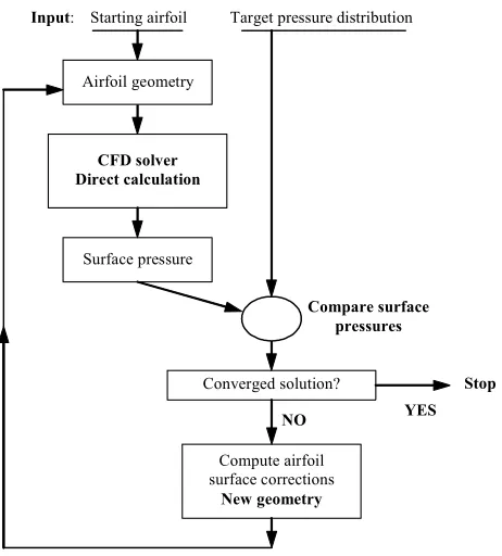
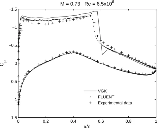
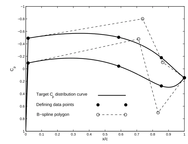
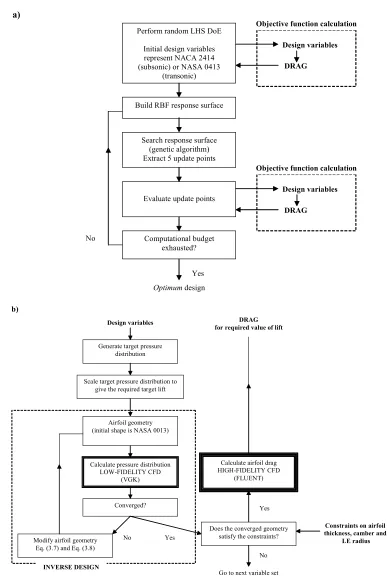
(7) List of Figures Figure 1-1. Future aircraft concepts. (a) A blended wing-body aircraft. (b) The supersonic biplane. .....................5. Figure 1-2 An airfoil design parameterization example. As the number of design variables is increased, there is an increase in both the level of local control and the complexity of the optimization task. ................................7 Figure 2-1. Example of a cubic Bézier curve. ........................................................................................................13. Figure 2-2. Example of an interpolating B-spline of degree three. ........................................................................15. Figure 2-3. Flowchart illustrating the design search and optimization process......................................................21. Figure 2-4. Flowchart illustrating a residual-correction type inverse design process. ...........................................26. Figure 3-1. A localized change in surface pressure has a global effect on the corresponding airfoil shape...........30. Figure 3-2. Flowchart illustrating the proposed EMFID design search process.....................................................31. Figure 3-3. The NASA LS(1)-0013 airfoil, and a variation of this shape featuring a sharp trailing edge. ............38. Figure 3-4 Comparison of pressure distributions generated using the FLUENT and VGK CFD solvers, for the NASA LS(1)-0013 airfoil. These are also compared against experimental data. ..............................................39 Figure 3-5 Comparison of pressure distributions predicted by the FLUENT and VGK solvers for the RAE2822 airfoil, shown with experimental data................................................................................................................40 Figure 3-6. Flowchart illustrating the benchmark (direct) design search strategy. ................................................42. Figure 3-7 13-variable airfoil geometry parameterization for the benchmark method using polynomial splines, showing control point degrees of freedom.........................................................................................................44 Figure 3-8 Six-variable airfoil parameterization for the benchmark method using B-splines, showing control point degrees of freedom. ..................................................................................................................................45 Figure 3-9. Parameterization of a subsonic Cp distribution using B-spline curves. ...............................................48. Figure 3-10 Pressure distributions generated in an objective calculation in EMFID, for the NASA LS(1)-0413 airfoil. .............................................................................................................................................................49 Figure 3-11 shock.. An example of a parameterized target pressure distribution, showing the two variables defining a .............................................................................................................................................................50. Figure 3-12 The error between the target and computed pressure distributions at the end of the inverse process, plotted against relaxation factor magnitude. ......................................................................................................54 Figure 3-13. Number of iterations required for inverse design, plotted against relaxation magnitude. ...................54. Figure 3-14. A converged inverse design result. The target is the Cp distribution for NACA 0012. .......................55. Figure 3-15 Comparison of geometries for a converged inverse design process, showing the design result and the shape corresponding to the target Cp profile......................................................................................................55 Figure 3-16 The NACA 2414 airfoil, and representations of this shape using the two benchmark parameterizations...............................................................................................................................................58 Figure 3-17 (a) Pressure distribution for the NACA 2414 airfoil, calculated using VGK, the representation of this profile using the subsonic EMFID parameterization and the inverse design result. (b) The NACA 2414 airfoil and the shape resulting from inverse design on the parameterized target. ..............................................58 Figure 3-18 The NASA LS(1)-0413 airfoil, and representations of this shape using the two benchmark parameterizations...............................................................................................................................................59 Figure 3-19 (a) Pressure distribution for the NASA LS(1)-0413 airfoil, calculated using VGK, the representation of this profile using the transonic EMFID parameterization and the inverse design result. (b) The NASA LS(1)-0413 airfoil and the shape resulting from inverse design on the parameterized target............................59 Figure 3-20 Detailed flowcharts: a) The optimization strategy used by the benchmark and EMFID methods, b) an objective function evaluation in EMFID. ..........................................................................................................62. vi.

(8) Figure 4-1. The five optimization histories for the benchmark and EMFID methods. ..........................................66. Figure 4-2 Final five geometries generated by the benchmark method. The lower figure shows the airfoils on equally scaled axes. ...........................................................................................................................................67 Figure 4-3. Final five geometries generated by the EMFID method......................................................................68. Figure 4-4 Comparison of the best performing geometry from each of the two methods, shown with two NASA low-speed airfoils of 13% thickness. .................................................................................................................70 Figure 4-5 (a) The optimized target pressure distribution, profile achieved during inverse design and profile output from FLUENT. (b) Pressure distributions due to the best performing EMFID and benchmark geometry, and the NASA LS(1)-0413 shape. .....................................................................................................................70 Figure 4-6 Lift-drag polar plot for the best designs from the benchmark and EMFID methods, shown with FLUENT results for two NASA airfoils. ...........................................................................................................71 Figure 4-7 Lift vs. angle of attack for the best designs from the benchmark and EMFID methods, shown with FLUENT results for two NASA airfoils. ...........................................................................................................72 Figure 4-8. The five optimization histories for the benchmark method using the six-variable parameterization. .73. Figure 4-9. Final five geometries generated by the six-variable benchmark method.............................................74. Figure 4-10. The five optimization histories for the benchmark and EMFID methods, for transonic airfoil design. .. .............................................................................................................................................................77. Figure 4-11. Final five geometries generated by the benchmark method, for transonic airfoil design. ...................78. Figure 4-12. Final five geometries resulting from the transonic EMFID method....................................................79. Figure 4-13 Comparison of the best performing geometry from each of the two methods, shown with supercritical airfoils NASA SC(2)-0712 and RAE 2822........................................................................................................80 Figure 4-14 (a) The optimized target pressure distribution , profile achieved during inverse design and profile output from FLUENT. (b) Pressure distributions due to the best performing EMFID and benchmark geometry, and the NASA SC(2)-0712 shape. .....................................................................................................................80 Figure 4-15 The five optimization histories for the EMFID method using a transonic Cp parameterization, shown with the results from case study 3......................................................................................................................83 Figure 4-16. Final five geometries resulting from the eight-variable transonic EMFID method.............................85. Figure 4-17 Comparison of the best performing geometry from the six-variable (subsonic) and eight-variable (transonic) EMFID methods, shown with the NASA SC(2)-0712 supercritical airfoil. ....................................86 Figure 4-18 (a) The optimized target pressure distribution, profile achieved during inverse design and profile output from FLUENT. (b) Pressure distributions due to the best performing EMFID and benchmark geometry, and the NASA SC(2)-0712 shape. .....................................................................................................................86 Figure 4-19 Lift-drag polar plot for the best designs from the six- and eight-variable EMFID methods, shown with FLUENT results for the NASA SC(2)-0712 and RAE 2822 airfoils.................................................................87 Figure 4-20 Lift vs. angle of attack for the best designs from the six- and eight-variable EMFID methods, shown with FLUENT results for the NASA SC(2)-0712 and RAE 2822 airfoils.........................................................88 Figure 5-1. An aircraft wake vortex study performed by NASA. ..........................................................................96. Figure 5-2. A racing car front wing, featuring end plates. .....................................................................................98. Figure 5-3 Examples of winglets on modern commercial aircraft (a) McDonnell Douglas MD-11 (b) Boeing 747-400, with a B747 freighter in the background. ...........................................................................................98 Figure 5-4. Example of a blended winglet on the Boeing 737-800........................................................................99. Figure 5-5. Example of a wing-tip fence on the Airbus A319. ..............................................................................99. Figure 5-6. Illustration showing the planform geometry of the raked wing-tip on the Boeing 767-400..............100. Figure 5-7 Surface pressure distribution for the ONERA-M6 wing at 99% span, showing the experimental data with viscous and inviscid results from FLUENT and VSAERO. ....................................................................103 Figure 5-8. Diagram illustrating the five gross wing-tip design variables, as listed in Table 5-1. .......................107. vii.

(9) Figure 5-9 An example of a wing-tip device generated using a parameterization of the trailing edge chord distribution. (a) Planform view on equally scaled axes. (b) A close-up view of the wing tip region. .............108 Figure 5-10 Comparison of lift profiles generated using FLUENT and VSAERO for the ONERA-M6 wing. These are compared with the elliptic distribution. .....................................................................................................111 Figure 5-11 (a) The best geometry from the 50 point DoE set. (b) Geometry resulting from inverse design, in which the target flow feature is the winglet lift profile of the geometry in (a). ...............................................113 Figure 5-12 The spanwise lift profile for the best winglet design in the DoE. Also shown is the inverse design result when the winglet portion is used as a target...........................................................................................114 Figure 5-13 Design and target geometries, and corresponging lift profiles, after 1, 10 and 27 inverse design iterations. .........................................................................................................................................................117 Figure 5-14. Flowchart illustrating the benchmark design search method.............................................................118. Figure 5-15 (a) Parameterization of the wing-tip chord distribution, (b) Discretization of the chord function and linear intepolation, (c) interpolation using a Catmull-Rom spline in GRIDGEN. ...........................................119 Figure 5-16. Flowchart illustrating the EMFID parameterization and design search process................................120. Figure 5-17. Parameterizations of the wing-tip device lift profile using (a) a quadratic and (b) a cubic polynomial. . ...........................................................................................................................................................122. Figure 5-18 Comparison of initial geometries used in the design searches, showing the benchmark parameterization and representations of this using the two EMFID parameterizations...................................125 Figure 6-1 Optimization-iteration histories for the benchmark and EMFID methods, showing traces for the threeand four-variable EMFID computations. Drag is calculated using the Euler FLUENT analysis. ...................129 Figure 6-2 (a) Planform view of the best geometry resulting from each of the five benchmark computations (shown on equally scaled axes). (b) A close-up view of the wing-tip region. .................................................132 Figure 6-3 (a) Planform view of the best geometry resulting from each of the five EMFID computations using the three-variable (quadratic) parameterization (shown on equally scaled axes). (b) A close-up view of the wing-tip region.................................................................................................................................................132 Figure 6-4 (a) Planform view of the best geometry resulting from each of the five EMFID computations using the four-variable (cubic) parameterization (shown on equally scaled axes). (b) A close-up view of the wing-tip region. ...........................................................................................................................................................133 Figure 6-5 Comparison of the best designs generated using the benchmark and EMFID parameterization methods............................................................................................................................................................134 Figure 6-6 Optimization-iteration histories for the benchmark and EMFID methods. Drag is calculated using the RANS FLUENT analysis.................................................................................................................................136 Figure 6-7 (a) Planform view of the best geometry resulting from each of the five benchmark computations (shown on equally scaled axes). (b) A close-up view of the wing-tip region. .................................................137 Figure 6-8 Illustration of the best chord distribution resulting from the benchmark method, showing the control points and the interpolating Catmull-Rom spline. ...........................................................................................138 Figure 6-9 (a) Planform view of the best geometry resulting from each of the five EMFID computations (shown on equally scaled axes). (b) A close-up view of the wing-tip region...............................................................139 Figure 6-10. Comparison of the best geometry generated using the EMFID and benchmark methods. ................140. Figure 6-11 Lift distributions predicted by VSAERO, showing the lift profile for the best benchmark design from Case 5, a least-square fit of the cubic curve, and the inverse design result. (a) The entire wing lift distribution. (b) A close-up view of the profile over the wing-tip. ......................................................................................141 Figure 6-12 The best benchmark geometry from Case 5, and the geometry resulting from inverse design. (a) Shown on equally scaled axes. (b) A close-up view of the wing-tip region. ...................................................142 Figure 6-13 Lift distributions predicted by VSAERO, showing the lift profile for the best benchmark design from Case 6, a least-square fit of the cubic curve, and the inverse design result. (a) The entire wing lift distribution. (b) A close-up view of the profile over the wing-tip. ......................................................................................143. viii.

(10) Figure 6-14 The best benchmark geometry from Case 6, and the geometry resulting from inverse design. (a) Shown on equally scaled axes. (b) A close-up view of the wing-tip region. ...................................................143 Figure 6-15 The lift profile optimized by the EMFID process, shown with the profile obtained after the geometry is repaired. Also shown is the best benchmark profile.....................................................................................144 Figure 6-16 VSAERO lift profile for the best EMFID design from case study 6, shown with the cubic target profile optimized to minimize the difference to the optimum design. .............................................................145 Figure 6-17 The EMFID geometry which was found to most closely match the best EMFID design. This was generated using the EMFID parameterization but without implementing the repair operation. (a) Shown on equally scaled axes. (b) A close-up view of the wing-tip region. ....................................................................146 Figure 6-18 Optimization-iteration histories for the EMFID and benchmark methods, showing the result when the EMFID search is run without the constraints on geometry..............................................................................147 Figure 6-19 The best design found when the EMFID method is run without the constraints on geometry, shown with the best result from case study 6. (a) Shown on equally scaled axes. (b) A close-up view of the wing-tip region. ...........................................................................................................................................................147 Figure 6-20 The best wing-tip design generated using the EMFID method, shown with a representation of this design using a four-variable Catmull-Rom spline. ..........................................................................................149 Figure A1-1. Wall y+ for the subsonic airfoil FLUENT analysis. ......................................................................161. Figure A1-2 Velocity in the x direction versus z co-ordinate at x=0.4, showing the growth of cells normal to the airfoil surface...................................................................................................................................................162 Figure A1-3. Variation of drag as the domain size is increased, showing the tolerance of acceptable accuracy. .... ......................................................................................................................................................163. Figure A1-4 Variation of drag as the number of surface cells is increased, showing the tolerance of acceptable accuracy. ......................................................................................................................................................164 Figure A1-5. The final 2-D subsonic airfoil mesh..............................................................................................164. Figure A1-6. Convergence of the drag coefficient during the FLUENT solution procedure. ............................165. Figure A2-1. Wall y+ for the transonic airfoil FLUENT analysis. .....................................................................169. Figure A2-2. Variation of drag as the domain size is increased, showing the tolerance of acceptable accuracy. .... ......................................................................................................................................................170. Figure A2-3 Variation of drag as the number of surface cells is increased, showing the tolerance of acceptable accuracy. ......................................................................................................................................................171 Figure A2-4 Surface pressure distributions for different FLUENT mesh configurations, varying the number of cells defining the airfoil surface.......................................................................................................................171 Figure A2-5 Convergence of the drag coefficient during the FLUENT solution procedure, for the transonic airfoil analysis..................................................................................................................................................172 Figure B-1 Final 3-D wing RANS analysis mesh. (a) View of constant ε planes through the flow domain. (b) View of constant η planes through the flow domain. (c) View of constant ζ planes through the flow domain. (d) Planform view of the wing surface mesh. ..................................................................................................177 Figure B-2. Wall y+ for a FLUENT analysis of the ONERA-M6 wing. ...............................................................178. Figure B-3. Variation of drag as the domain size is increased, showing the tolerance of acceptable accuracy....179. Figure B-4 (a) Variation of drag as the number of chordwise cells is increased. (b) Variation of drag as the number of spanwise cells is increased. ............................................................................................................179 Figure B-5. Convergence of the drag coefficient during the FLUENT RANS solution procedure. .....................180. Figure B-6 Variation in the FLUENT Euler drag as the first cell height is increased (this reduces the total number of mesh cells)...................................................................................................................................................185. ix.

(11) Figure B-7. Panelling scheme used in VSAERO. (a) Planform view. (b) Front isometric view. .........................187. Figure B-8 (a) Number of wake relaxation iterations vs. VSAERO drag. (b) Number of viscous iterations vs. VSAERO drag. ................................................................................................................................................188 Figure B-9 Surface pressure distributions over the ONERA-M6 wing at six spanwise stations, predicted by the FLUENT RANS analysis and viscous VSAERO simulations.........................................................................189 Figure C-1 The initial extended ONERA-M6 wing geometry (above). FLUENT prediction of velocity vectors in the region of the tip vortex at X=4m (above right). Vorticity contours (right) from FLUENT at the X=4 plane, showing a black cross corresponding to the vortex centre predicted by VSAERO. ........................................193 Figure C-2 The best geometry from the 50 point DoE set (above). FLUENT prediction of velocity vectors in the region of the tip vortex at X=4m (above right). Vorticity contours (right) from FLUENT at the X=4 plane, showing a black cross corresponding to the vortex centre predicted by VSAERO. ........................................193 Figure C-3 The worst geometry from the 50 point DoE set (above). FLUENT prediction of velocity vectors in the region of the tip vortex at X=4m (above right). Vorticity contours (right) from FLUENT at the X=4 plane, showing a black cross corresponding to the vortex centre predicted by VSAERO. ........................................194 Figure C-4. FLUENT predictions for drag and maximum vorticity for all 50 designs, sorted by the drag values. .... ...........................................................................................................................................................195. Figure C-5 (a) FLUENT predictions of drag and circulation for all 50 design points, where the points have been sorted in ascending drag order, (b) FLUENT drag predictions and VSAERO circulation results for the same designs. ...........................................................................................................................................................196 The best benchmark geometry from case study 6 (RANS simulations), shown with two variants of Figure D-1 this design. (a) On equally scaled axes. (b) A close-up view of the wing-tip region.......................................198 Figure D-2 Flow visualization showing streamlines emitted from the trailing edge of the wing-tip device, for the best design from case study 6. (a) planform view, (b) front isometric view....................................................200 Figure D-3 Flow visualization showing streamlines emitted from the trailing edge of the wing-tip device, for a design with the tip chord minimized. (a) planform view, (b) front isometric view. ........................................200 Figure F-1. The optimization strategy. .................................................................................................................207. x.

(12) List of Tables Table 4-1 Airfoil design data for the best geometries resulting from the five benchmark design searches: maximum thickness, maximum camber, angle of attack, lift coefficient and drag coefficient..........................67 Table 4-2 Airfoil design data for the best geometries resulting from the five EMFID design searches: maximum thickness, maximum camber, angle of attack, lift coefficient and drag coefficient...........................................68 Table 4-3 Airfoil design data for the five geometries resulting from the six-variable benchmark design search: maximum thickness, maximum camber, angle of attack, lift coefficient and drag coefficient..........................74 Table 4-4 Airfoil design data for the five geometries resulting from the transonic benchmark design search: maximum thickness, maximum camber, angle of attack, lift coefficient and drag coefficient..........................78 Table 4-5 Airfoil design data for the five geometries resulting from the transonic EMFID design search: maximum thickness, maximum camber, angle of attack, lift coefficient and drag coefficient..........................79 Table 4-6 Airfoil design data for the five geometries resulting from the eight-variable transonic EMFID design search: maximum thickness, maximum camber, angle of attack, lift coefficient and drag coefficient..............85 Table 4-7. Summary of the 2-D airfoil case studies..............................................................................................89. Table 5-1. Gross wing-tip device design variables. ............................................................................................107. Table 6-1 Design objective (drag coefficient calculated using FLUENT Euler simulations) for the five best designs resulting from the benchmark and EMFID methods...........................................................................131 Table 6-2 Design objective (drag coefficient calculated using RANS FLUENT) for the five best designs resulting from the benchmark and EMFID methods........................................................................................137 Table 7-1. Summary of the case studies reported in this thesis. .........................................................................153. Table A1-1. Information regarding the setup of the subsonic 2-D airfoil CFD solver. ....................................165. Table A2-1. Information regarding the setup of the transonic 2-D airfoil CFD solver.....................................172. Table B-1. Information regarding the setup of the 3-D wing RANS analysis.....................................................181. Table B-2. Information regarding the setup of the 3-D wing Euler analysis.......................................................186. Table C-1 Data relating to the wing-tip vortex for the initial, best and worst designs in the 50 point DoE set, as predicted by FLUENT and VSAERO..............................................................................................................194 Table D-1 D-1.. Drag coefficients calculated using FLUENT Euler and RANS analyses for the three designs in Figure ...........................................................................................................................................................198. xi.

(13) Acknowledgements I am sincerely grateful to many people for their guidance and support throughout my three years of study in the Computational Engineering and Design research group. The work in this thesis has been funded by a studentship from the University of Southampton School of Engineering Sciences, which is gratefully received. The support and guidance from the project supervisors, Dr. Neil Bressloff and Professor Andy Keane, has been fabulous, and I could not have wished for a better supervisory team. In addition, the initial leadership from Robert Lewis at Advantage CFD is greatly appreciated. My deepest thanks go to many people in the research group for their emotional, technical and editorial support, as well as their friendship; in particular: Alex and Jen Forrester, Nici Hoyle, Tony Scurr, András Sóbester, Praveen Thokala, David Toal and Narcis Ursache. To generate the results presented in this thesis has required over 24000 hours of run time on the Microsoft Compute Cluster; I am enormously grateful to Ivan Voutchkov for his hard work in maintaining the cluster, and for the countless occasions when I have gone to him for help. Following my internship at the Institute of Fluid Science at Tohoku University, I am grateful to Professor Shigeru Obayashi for kindly accommodating me in his research group and Nao Konohara for her helpful support during my stay. Finally, but not least, I want to thank my family. In particular, I thank my Dad for offering so much guidance throughout my education, and I thank Sarah for her unending encouragement.. xii.

(14) Declaration of Authorship. I, Thomas Robin Barrett, declare that the thesis entitled. “Aerodynamic Design Optimization Using Flow Feature Parameterization”. and the work presented in the thesis are both my own, and have been generated by me as the result of my own original research. I confirm that: •. this work was done wholly while in candidature for a research degree at this University;. •. where any part of this thesis has previously been submitted for a degree or any other qualification at this University or any other institution, this has been clearly stated;. •. where I have consulted the published work of others, this is always clearly attributed;. •. where I have quoted from the work of others, the source is always given. With the exception of such quotations, this thesis is entirely my own work;. •. I have acknowledged all main sources of help;. •. where the thesis is based on work done by myself jointly with others, I have made clear exactly what was done by others and what I have contributed myself;. •. parts of this work have been published as: Barrett et al. [2006a], Barrett et al. [2006b], Barrett et al. [2006c].. In addition, the thesis conforms, where possible, to British standard BS 4821:1990.. Signed:. Date:. November, 2007. xiii.

(15) Nomenclature Listed below are the definitions commonly used in this thesis.. x. =. geometrical ordinate in the streamwise direction, for two-dimensional flow. z. =. geometrical ordinate in the vertical direction, for two-dimensional flow. X. =. geometrical ordinate in the streamwise direction, for three-dimensional flow. Y. =. geometrical ordinate in the spanwise direction, for three-dimensional flow. Z. =. geometrical ordinate in the vertical direction, for three-dimensional flow. Μ. =. flow speed Mach number. Re. =. flow Reynolds number. α. =. angle of attack. Cp. =. pressure coefficient. cd. =. airfoil drag coefficient, normalized with respect to chord. cl. =. airfoil lift coefficient, normalized with respect to chord. c. =. airfoil chord. zt max =. airfoil maximum thickness. zc max =. airfoil maximum mean thickness (maximum camber). rLE. =. airfoil leading edge radius. CD. =. wing drag coefficient, normalized with respect to wing projected area. CL. =. wing lift coefficient, normalized with respect to wing projected area. xiv.

(16) Chapter 1. Introduction. “As we have moved from the great pioneers, such as Lanchester, to the modern age of sophisticated computational methods and integrated ways of working, so we have moved from the ‘art of compromise’ to the ‘science of optimisation’.”. The above quotation is taken from a lecture given by Jeff Jupp of Airbus (Jupp [2001]). It portrays succinctly that the process of design is one of compromise. In a modern aircraft design project, these compromises can be vastly complex, but they are not beyond reasoning when modern computational methods are employed in the design process. This design process, and indeed this thesis, is multi-faceted, and concerns aerodynamics analysis, parametric modelling techniques and optimization.. 1.1. The Role of Aerodynamics in Design. Historically, the study of aerodynamics has been motivated to a large extent by the dream of achieving and perfecting the act of manned powered flight. As recently as the late 19th century, the flight of birds and insects was thought by some to rely on a mythical “vital force”, and fierce debate raged amongst the scientific community as to whether such motion could be achieved by an inanimate object. Wilbur Wright commented similarly in 1901 “nobody will fly for a thousand years”, but two years later thanks to their persistence the Wright brothers achieved their dream. Aerodynamics concerns the prediction of forces and moments acting on a body, when the body is immersed in a fluid (usually air) with relative velocity. The motion of a fluid over a solid body gives rise to two basic flow phenomena: the pressure distribution acting normal to the surface and the shear stress distribution acting tangential to the surface due to the. 1.

(17) Introduction. 2. viscosity of the fluid. Knowledge of these flow phenomena permits the prediction of the net forces and moments on the body, and this is the key interest of an engineer. Engineers strive to use their knowledge of aerodynamics in order to design improved products. However, design decisions are rarely based on experience alone, and rely additionally on the use of some form of analysis. The Wright brothers built their own wind tunnel in their bicycle shop, performing a series of methodical experiments with airfoil and planform geometries in the quest for a more efficient wing design. The scale and complexity of modern aircraft design projects and analysis techniques far exceeds the efforts of the Wrights, but after more than 100 years the same principles of engineering design practice still apply. Classical analysis of finite wings and airfoils (infinite wings) began with the solution of potential flow equations, i.e., the closed form solution for inviscid, irrotational, incompressible flow. This was performed with hand calculations until the arrival of the modern digital computer, which allowed large calculations to be rapidly performed. By the 1960’s, computational fluid dynamics (CFD) approaches such as the source panel method were standard tools of the aerospace industry. Further development of CFD solution schemes allowed the iterative solution of transonic potential flow, the Euler equations, and subsequently the Reynolds averaged Navier-Stokes (RANS) equations. Modern research into design oriented CFD focuses on turbulence simulation and accurate drag prediction, as well as reducing computational expense. CFD simulations are relied upon heavily in modern aircraft design projects. Because this is a relatively inexpensive task compared to experimental wind-tunnel testing, CFD can be performed on a large scale and can be easily accessed by all the designers. Typically, varying levels of CFD fidelity and capability are used at different stages in the design process. At the concept design stage, the objective is to assess the technical and economic feasibility of the potential product as a whole, and this consideration should encompass all aspects of the design and its impact on the user. This study is often based on previous designs, and so empirical and calibrated CFD analyses are commonly employed. At the preliminary and detailed design stages the product is broken down into the design of its component parts; higher fidelity analysis methods are used in order to model the relevant flow features in more detail, and obtain a more accurate figure for the predicted drag. The use of more expensive and complex flow simulations in preliminary design means that much of the engineering time is spent in pre-processing and postprocessing the analysis. The decision of what modifications should be made to the design is typically a manual one, and this is not always obvious based on the results of CFD. There are invariably compromises to be made with each design decision; there could be conflicting aerodynamic load requirements, and structural issues often lead to further compromises in the aerodynamic performance..

(18) Introduction. 3. Thus, the need to perform a more systematic exploration of engineering compromises, and accelerate the design process, has lead to the increasing use of automated optimization methods. Optimization as a subject in mathematics is very old, but its application in aerodynamic design problems only began in earnest following the widespread use of the modern digital computer. At its most fundamental, optimization is the search for a set of inputs to a function, known as the objective function, that result in that function taking its minimum possible value, or, conversely, its maximum possible value for a maximization problem. Despite the optimization techniques being carried over into an aerospace design context, such functions are rarely optimized per se. Rather, the non-linear nature of CFD analysis and the requirement for a large and multi-dimensional search space means that this is an exercise in design improvement, hence the term design search and optimization (DSO) is used. This line of reasoning is shared by van Egmond [1990]: “Expectations of achieving the absolute best design invariably lead to maximum disappointment”. In addition, the inputs to an objective function and the computational model can never be all-encompassing, i.e., there will always be real life factors not taken into account in the design search process. Therefore, automated optimization processes are used in industrial situations to complement and accelerate the work of the engineer. A fundamental requirement for performing optimization is a parametric description of the design; for aerodynamic design this parameterization typically involves inputs relating to the external geometry. The selection of an appropriate parameterization is a key factor in the successful application of DSO methods, and this is the focus of this thesis.. 1.2. The Role of Parameterization in Design. The basic process of design has been described as the making of decisions that change the product definition (Keane and Nair [2005]). In aerodynamic design, these decisions are made based on the results of the aforementioned aerodynamic analysis. The product definition, in its most traditional form, is an engineering drawing communicating the physical dimensions and geometrical features of the product. However, such a primitive description does not readily allow measured and reproducible changes, and certainly prevents automated changes using an optimization algorithm. The need for an efficient and systematic approach to aerodynamic design was recognized in the 1930’s by the designers of the NACA1. 1. National Advisory Committee for Aeronautics, which subsequently became the National Aeronautics and Space Administration (NASA)..

(19) Introduction. 4. 4-digit airfoils (Jacobs et al. [1933]). The designers used a series of successful airfoil shapes to generate one of the earliest examples of a parametric model, i.e., a mathematical description which allows a design to be defined using one or more design variables. Among these design variables are the airfoil thickness and camber quantities. This model facilitates intuitive and precisely measured changes to the shape, and leads to a methodical design process. In many fields of modern engineering design, the required product definition is becoming increasingly more complex, and designers are forced to adhere to ever more demanding time and budget constraints. The former is particularly true in aerodynamic shape design, where detailed and subtle design changes are often necessary to minimize drag or control a separation point, for example. Thus, a significant research effort has gone into investigating more sophisticated techniques for representing and manipulating designs. At present, the parameterization techniques used in aerospace design can be split into two broad classes: computer aided design (CAD) based methods, and analytical techniques. Modern CAD software is becoming increasingly sophisticated, and is typically capable of quite complex parametric modelling tasks using non-uniform rational B-spline (NURBS) curves and surfaces. CAD is also very accessible to the designer, allowing the input of design data from external software and the export of geometry and mesh data to a CFD pre-processor. There are also many powerful analytical methods which have not yet been adopted in CAD packages. These include basis function methods, partial differential equation methods and free-form deformation. An introduction to the most commonly used parameterization techniques follows in Chapter 2. A parameterization scheme can be set up to perform global changes in shape or local modifications, or in some cases, both (Hoyle [2006]). In the design process, a global method is typically used in the initial concept stage, while increasingly local techniques are employed at subsequent stages (Keane and Nair [2005]). An example of a global technique is a NURBS representation of a full aircraft wing-body configuration; this can typically perform large modifications to the design and is not constrained with respect to its overall form. The ability to perform global shape modifications is a key attribute for parameterization schemes employed for conceptual design tasks. An ability to consider radically different designs is becoming increasingly important, as designers are forced to consider new concepts in a bid to reduce the environmental impact of passenger aircraft. The main aircraft emissions targets set out by the European commission to be achieved by 2020 are a 50% reduction in carbon dioxide emissions per passenger kilometre, and an 80% cut in nitrous oxide emissions (Reneaux [2004]). Drag reduction can contribute significantly to this effort. Aircraft manufacturers therefore have a responsibility to pursue revolutionary.

(20) Original in colour. Introduction. 5. concepts such as the blended wing-body and the supersonic biplane (Yamashita et al. [2007]), which are illustrated in Figure 1-1 (a) and (b), respectively. Both of these concepts promise to dramatically reduce drag; the blended wing body could greatly improve the lift to drag ratio, while the supersonic biplane features very little wave drag at cruise conditions. These examples emphasize the importance of considering a global range of designs at the conceptual stage.. (a) Figure 1-1. (b). Future aircraft concepts. (a) A blended wing-body aircraft. (b) The supersonic biplane.. In addition to providing global shape manipulation, a parameterization can be used to perform more local surface modifications. Local techniques are able to apply detailed modifications to a specific area of the product. Examples include the use of NURBS control points and bump functions. Provided the constraints on a design problem allow it, local modifications can also result in radically different designs. However, some techniques, such as the above NACA airfoil definition, are based on a set of existing designs, and thus the generated designs are generally evolutionary relative to the input set. Parameterization and shape control techniques have undergone extensive development, and an impressive level of local control can be achieved. However, increasing the degree of surface control usually entails an increase in the number of design variables. This increase in dimensionality increases the complexity of the design task, and when automatic optimization is employed this equates to an increase in the computational cost of a design search. Thus, there is a need for parsimonious parameterization techniques in order to minimize this cost..

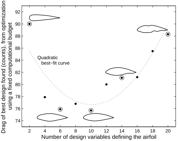
(21) Introduction. 1.3. 6. The Need for Efficiency in Design. Despite advances in CFD simulations, computing power and optimization strategies, the computational expense of high-fidelity CFD means that more efficient design optimization methods are still sought after for use in aerodynamic design. A reduction in the number of input parameters as a result of improved parametric modelling is a common contributor to this efficiency. As previously mentioned, this number of input parameters can be large when manipulating geometry, in order to obtain the detail and smoothness required for high-fidelity flow analysis. Additionally, many large-budget, state-of-the-art aerospace design projects result in highly complex and intricate geometries. However, an increase in model complexity usually comes with an increased cost in performing the design search. Thus, the setup of a parameterization scheme is an interesting compromise between achieving a sufficient level of detail and local control, and minimizing the complexity of the design task. Figure 1-2 illustrates this compromise, by considering the problem of minimizing the drag of an airfoil. A design search is set up in which the airfoil is parameterized using a spline curve method, where the design variables are the positions of control points on the airfoil surface. The drag is determined using a lowfidelity potential flow solver and a genetic algorithm (GA) is employed to search for low-drag designs; note that any optimization algorithm could be used in this example problem. This design search is run ten times, using a different number of variables to define the airfoil shape at each attempt and using the same number of GA iterations, representing a fixed computational budget. Figure 1-2 plots the number of variables used versus the best drag result obtained during the search, also showing some of the optimized airfoil geometries. It can be seen that when 2 design variables are employed the poor degree of local control severely limits the ability to generate low drag designs, but the airfoil shape is regular and smooth. In contrast, when the airfoil is defined using 20 variables, it is clearly possible to achieve very good local control, but the immense complexity of this design search has resulted in a best design which lacks smoothness, and therefore it too has a rather high drag. Many thousands of design iterations, and a large computational budget, would be required for this design search to converge onto a truly optimal design. In this design example, the best compromise is achieved when 10 variables are employed for optimization, since this provides sufficient local control but also converges sufficiently quickly to reach a low-drag airfoil shape. This simple example demonstrates the need for efficient parameterization schemes, which are able to generate detailed and complex changes in shape, but which use a relatively small number of design variables to minimize the cost of a design search..

(22) 7. Drag of best design found (counts), from optimization using a fixed computational budget. Introduction. 92 90 88 86 Quadratic best−fit curve. 84 82 80 78 76 74 2. 4. 6. 8. 10. 12. 14. 16. 18. 20. Number of design variables defining the airfoil. Figure 1-2 An airfoil design parameterization example. As the number of design variables is increased, there is an increase in both the level of local control and the complexity of the optimization task.. A great advantage of CFD is the ability to calculate pressure and velocity data at any point in the discretized domain, be this on the body surface or in the off-surface flow. This data can be used to extract information relating to individual flow features such as induced vortices, separation, or the variation of surface pressure or aerodynamic forces. These flow features can be implicitly linked to the analysed geometry. However, while the definition of geometry can be very complex, one can imagine that when subjected to a flow field the resulting flow features are not necessarily so complex. For example, in minimizing the induced drag of a wing one might aim for a simple elliptical lift distribution, while the corresponding shape, for a given flow field, could turn out to be rather more complicated. In such situations, one can postulate that the flow features surrounding the component are potentially simpler to represent parametrically than the geometry. Also, since varying the flow features is likely to have an effect on the entire geometry under analysis, a simple parameterization of flow features may be able to produce quite complex geometrical modifications. Further, such a parameterization will perceivably have an intuitive effect on aerodynamic forces, such as lift and drag. Of course, by specifying flow features, the designer is then tasked with determining the geometry which realizes these flow features for the given flow conditions. The specification of flow features and subsequent realization of the required geometry is not a new idea. So-called inverse design methods have been used widely, particularly in the context of designing an airfoil which generates a prescribed surface pressure distribution; see for example, Dulikravich [1990] or Drela [1989]. The design of flow features is.

(23) Introduction. 8. not an intuitive concept, perhaps because aerodynamic effects are invisible whereas engineers are more familiar with geometry manipulation. However, the design of flow features is in some senses more logical; after all, it is the flow features which uniquely establish the forces on a body. The geometry is simply the means of achieving the required flow features. Despite the increasing importance of aesthetics, engineers are concerned rather less by what their product looks like; instead their efforts are focused on improving its performance. Inverse design has been used for various flow feature specifications (for example Qin et al. [2005] used the spanwise lift profile), but not principally as a means of reducing the dimensionality of design optimization problems. The aim of the work described in this thesis is to investigate the use of flow feature parameterization as a means of improving the efficiency of the design process. It is proposed that this technique can generate detailed and localized geometrical modifications while reducing the total number of defining design variables. The research does not focus on optimization algorithms or CFD techniques, but rather a method in which shape control, inverse design and optimization methods are combined in an attempt to accelerate the process of design. In this work, the application of such methods is to the aerodynamic design of 3-D aircraft wings and 2-D wing sections. Consistently, a comparison is made between two design strategies. The first is treated as a benchmark in aerodynamic shape optimization, in which the geometry is defined parametrically using a representative number of input parameters, and each design selected by the optimization process is analysed using high-fidelity CFD to give a measure of performance. The alternative approach uses a parameterization of flow features, since they can potentially be described using fewer inputs, combined with an inverse design step to recover the required geometry. Following inverse design, each design is evaluated identically to those in the benchmark process. This work is therefore a comparison between these two approaches to parameterization, and investigates the design performance of these methods given a fixed computational budget..

(24) Introduction. 1.4. 9. Thesis Outline. The purpose of thesis is to compare two different parameterization approaches for aerodynamic design, and to demonstrate their relative performance using practical examples. Therefore, the work makes frequent references to the disciplines of parametric modelling, CFD analysis, optimization algorithms and design strategies including inverse design. A background to these items is given in Chapter 2. In Chapter 3, the concept of flow feature parameterization is introduced, and areas of related work are identified. The proposed parameterization technique is first applied to the design of 2-D airfoils, and is evaluated relative to the benchmark process. The parameterized flow feature for this application is the airfoil surface pressure distribution. The setup of a comparison between the two design methods is described, detailing the parameterization techniques, optimization strategy, CFD analysis setup and inverse design. Chapter 4 reports the results of four case studies for 2-D airfoil design. The objective of the design searches is to minimize the total drag of the airfoil at a single operating point. Drag is calculated using RANS analyses; in the first two case studies a subsonic flow regime is specified, and in two further case studies a transonic flow regime is used. The results from these case studies are analysed in detail and conclusions are drawn. In Chapter 5, the proposed parameterization method is implemented in a 3-D design scenario. The task is to design a wing-tip device with the objective of minimizing drag. A background to the use of wing-tip devices is documented. Following this, a study is described which investigates an appropriate flow feature to parameterize for this 3-D design problem. The chosen geometry description is the trailing edge chord distribution, and the parameterized flow feature is the spanwise lift distribution. The setup of a comparison between design searches using the flow feature based parameterization and the geometrybased parameterization is described. Chapter 6 reports two case studies for this 3-D wing-tip design task; in one the drag is calculated using Euler simulations, and the other uses RANS simulations. The results from these design searches are analysed and conclusions are drawn. In Chapter 7, the findings reported in Chapters 4 and 6 are scrutinized in a general sense. Key conclusions and contributions are listed. To finish, recommendations for future work are given describing how the work in this thesis could be taken further..

(25) Chapter 2. Current Practices in. Aerodynamic Design. The purpose of this thesis is to present a new approach to the design of components subjected to aerodynamic flows. The work exploits many other computational techniques which are well established and used routinely in design exercises. Before any alternative concept is presented, these current practices are discussed, forming a background to the methods used in later chapters. One of the key themes of this work is parameterization techniques; a number of examples are given below and their relative advantages and disadvantages are discussed. This chapter also outlines the key areas of CFD analysis and optimization algorithms, and introduces the concept of inverse design.. 2.1. Parameterization Techniques. Parameterization is the representation of the chosen physical characteristics of a design in terms of one or more numerical parameters, known as design variables. These design variables can be either continuously varying or discrete. Typically, such a parameterization is applied to geometry, describing changes to all or part of the design under scrutiny. Using a parametric description of a design, the job of the designer, or indeed, an optimization algorithm, is to select the values of the design variables which give an improved design performance. In engineering design, this selection process is based on the results of analysis, be this computational or experimental. Each variable has a range associated with it; collectively these ranges form the design space, with each design taking up a point in this space. At its lowest level, the NACA definition (described below) allows an airfoil to be described using only its camber and thickness quantities, allowing rapid design studies to be performed. In this case the use of only two variables permits a thorough search of the design space, but may not be able to manipulate the airfoil shape in sufficient detail to give the required performance gains. Conversely, a more detailed parameterization may yield improved performance but result in a more lengthy design search due to the higher dimensional search space. Thus, as demonstrated in Chapter 1, the choice of parameterization technique is often a trade-off between the detail and complexity required for a design and the budget of analysis calls. 10.

(26) Current Practices in Aerodynamic Design. 11. afforded. This has been the subject of extensive research, seeking for representations which reduce the number of design variables while retaining the ability to capture a global range of designs. A survey of many techniques used in the aerospace sector is given by Samareh [1999]. Below is an outline of a number of geometric parameterization techniques relevant to the current work.. 2.1.1. NACA Airfoils. During the 1930’s, NACA (National Advisory Committee for Aeronautics, which later became NASA) developed one of the earliest examples of geometric parameterization. The experimentally developed definition gives smooth and efficient airfoil shapes, and forms a family known famously as the NACA 4digit series. These airfoils have been heavily used in the aircraft industry, but are rarely used today having been replaced by more advanced CFD developed shapes. The 4-digit airfoil definition is described in the landmark NACA Report 460 (Jacobs et al. [1933]), and is summarized here. In this definition, the airfoil is specified using an expression for the camber line plus a thickness distribution either side of this line, forming the upper and lower surfaces in two-dimensional (x,z) coordinates. The camber line, zc, consists of one parabola from the leading edge to the point of maximum camber, and another parabola extending from this point to the trailing edge:  1 z c = z c max   (x ) 2  m.  (2 x m x c − ( x c) 2 )  . for. 0 ≤ x c ≤ xm ,.   1 (1 − 2 xm + 2 xm x c − ( x c) 2 ) for zc = zc max   (1 − x )2  m  . and. xm ≤ x c ≤ 1 .. (2.1). Here, zc max is the maximum camber and xm is the position of maximum camber as a fraction of the chord, c. The thickness distribution, zt, is a simple irrational polynomial function, the coefficients of which were found by fitting to a number of popular airfoils of the time: zt = 5 zt max (0.2969 x c − 0.1260 x c − 0.3537( x c)2 + 0.2843( x c)3 − 0.1015( x c)4 ) ,. (2.2). where z t max is the airfoil maximum thickness. The airfoil co-ordinates are given by xU = x − zt sin(θ ). zU = z c + z t cos( θ ). xL = x + zt sin(θ ). z L = z c − z t cos( θ ). ,. (2.3).

No results found