Analysis and development of iterative fast model control strategies for systems with constraints

(1)

University of Southern Queensland

Faculty of Engineering & Surveying

Analysis and Development of Iterative Fast

Model Control Strategies for Systems with

Constraints

A thesis submitted by

Sarang Ghude

M.Eng.Tech, B.Eng

in fulfilment of the requirements of

Doctor of Philosophy

(2)

Abstract

In this research, new fast model control strategies are developed and analysed. To avoid confusion with the competing directions taken by Predictive Control they have been named ‘Iterative Fast Model Control (IFMC) Strategies’. It has been shown that new IFMC strategies deliver near time optimal performance and have finite settling time. IFMC strategies that include various state constraints are also developed. The system responses and the Lyapunov stability have been analysed.

The possibility of extending IFMC strategies for systems up to an nth _order

is supported by development of IFMC strategies for 6th _{to 11}th _{order systems.}

Application of IFMC in a real life situation of Aircraft Lateral Control has been studied. Successful implementation of IFMC in a third order ball and beam experiment demonstrates its effectiveness practice. A performance comparison with other contemporary strategies showed that IFMC delivers performance with almost 45% improvement.

The purpose of any real time controller is to determine the drive that should be applied to the plant at each instant. In IFMC, this is performed with the aid of a fast model of the system that can run at a speed that may be a thousand or more times that of the system. Then a decision on plant input is made, based on the fast model behaviour. The input is constrained at both extremes, full positive and full negative.

(3)

Certification of Dissertation

I certify that the ideas, designs and experimental work, results, analyses and conclusions set out in this dissertation are entirely my own effort, except where otherwise indicated and acknowledged.

I further certify that the work is original and has not been previously submitted for assessment in any other course or institution, except where specifically stated.

Sarang Ghude 0050036313

Signature of Candidate

Date

ENDORSEMENT

Signature of Principal Supervisor

Date

Signature of Associate Supervisor

(4)

Acknowledgments

I consider myself fortunate to have had an opportunity to work with Prof. John Billingsley. He boosted my interest in research during my masters then helped me to become a better researcher through my PhD candidature. His guidance and support was not limited to just research but was extended to many other areas. I have learned a lot from him and I hope I’ll continue to learn in future also. I am grateful for his guidance, support and encouragement. “Thanks, John”.

I sincerely thank, Assoc. Prof. Paul Wen for his guidance during my studies. I am thankful to Faculty of Engineering and Surveying of USQ, for offering me scholarship during my candidature. I thank, Mr. Mark Phythian, Assoc. Prof. David Buttsworth and Mr. Steven Goh for offering me teaching assistantship from time to time. I also thank Mr. Dean Believeu for his technical support and friendship.

Playing guitar and cricket have provided much needed relaxation, thus, helping indirectly in my research. My guitar self-learning effort might have lost its vigour if the invaluable guidance and encouragement from Dr. Rabi Misra was not there. I will always cherish this ‘musical’ friendship. “Thanks a lot, Rabi”. I have learned a lot about playing cricket, at our cricket club that made me a better cricketer. A thanks would go to all my friends at the club, Thanks Uni-Bushchooks. I extend my thanks to all of my past and present friends at USQ and from home.

Last but most important, I express my deepest gratitude to my parents for their endless love, support and encouragement. This thesis is dedicated to my parents.

(5)

List of Figures

3.1 1968 Fast Model Predictive Control Strategy Curves:- 1: Predic-tions with full positive drive, 2: PredicPredic-tions with full negative drive, 3: Position x, 4: 10*Acceleration (a) . . . 23

3.2 1987 Fast Model Predictive Control Strategy Curves:- 1: Predic-tions with full positive drive, 2: PredicPredic-tions with full negative drive, 3: Position x, 4: 10*Acceleration (a) . . . 24

3.3 Iterative Fast Model Control Strategy Curves:- 1: Predictions with full positive drive, 2: Predictions with full negative drive, 3: Posi-tion x, 4: 10*Acceleration (a) . . . 25

3.4 Time optimality test result of Iterative Fast Model Control with Third Order System Curves:- 1: Predictions with full positive drive, 2: Predictions with full negative drive, 3: Position x, 4: 10*Acceleration (a), 5: 10*Backward journey of acceleration (a) fromx= 0,v = 0 and a= 0 . . . 26

3.5 Iterative Fast Model Control with Third Order System, termina-tion using error conditermina-tion. Curves:- 1: Predictermina-tions with full posi-tive drive, 2: Predictions with full negaposi-tive drive, 3: Position x, 4: 10*Acceleration (a), 5: 10*Backward journey of acceleration (a) fromx= 0,v = 0 and a= 0 . . . 28

(11)

LIST OF FIGURES x

3.7 Fast Model Control Strategy 1987 - Fourth Order System Curves:-1: Predictions with full positive drive, 2: Predictions with full

negative drive, 3: Positionx, 4: 10*Jerk (j) . . . 30

3.8 Iterative Fast Model Control - Fourth Order System Curves:- 1: Predictions with full positive drive, 2: Predictions with full nega-tive drive, 3: Position x, 4: 10*Jerk (j) . . . 31

3.9 Final values of State (position) for different strategies . . . 32

3.10 Color Plots IFMC Strategy with Smaller Steplength . . . 33

3.11 Color Plots of Final Variable Values . . . 34

3.12 Color Plots of Final Variable Values with new error for 2008 Strategy 35 3.13 Color Plots for time optimal performance of Iterative Fast Model Control Strategy . . . 37

4.1 Iterative Fast Model Control of a Second Order System Curves:-1: Predictions with full positive drive, 2: Predictions with full negative drive, 3: Positionx, 4: 2*Velocity (v) . . . 42

4.2 IFMC traces after time T when t− > t+ Curves:- 1: Prediction of position with full negative drive, 2: Prediction of position with full positive drive, 3: Prediction of velocity with full positive drive, 4: Prediction of velocity with full negative drive. . . 43

4.3 IFMC traces after time T whent−almost=t+ Curves:- 1: Predic-tion of posiPredic-tion with full negative drive, 2: PredicPredic-tion of posiPredic-tion with full positive drive, 3: Prediction of velocity with full positive drive, 4: Prediction of velocity with full negative drive . . . 44

4.4 IFMC curves after timest+=t−Curves:- 1: Predictions of position with full positive drive, 2: Predictions of position with full negative drive, 3: Plant Position, 4: Plant Velocity . . . 45

(12)

LIST OF FIGURES xi

4.6 Iterative Fast Model Control of a Third Order System 1: Pre-dictions with full positive drive, 2: PrePre-dictions with full negative drive, 3: Position x, 4: 10*Acceleration (a) . . . 49

4.7 3rd _{order IFMC traces after time T when} _t

−almost=t+

Curves:-1: Prediction of position with full negative drive, 2: Prediction of position with full positive drive, 3: Prediction of velocity with full positive drive, 4: Prediction of velocity with full negative drive, 5: Prediction of acceleration with full positive drive, 6: Prediction of acceleration with full negative drive . . . 50

4.8 The graph of variable x,variable a and input u . . . 53

4.9 Simulation of Iterative Fast Model Control when t−=t+ second time 54

4.10 Simulation of Iterative Fast Model Control with a Fourth Order System Curves:- 1: Predictions with full positive drive, 2: Predic-tions with full negative drive, 3: Position x, 4: 10*Jerk (j) . . . . 56

4.11 Simulation of Iterative Fast Model Control with a Fifth Order Sys-tem Curves:- 1: Predictions with full positive drive, 2: Predictions with full negative drive, 3: Position x, 5: 10*Rate of jerk k . . . . 57

4.12 Simulation of Iterative Fast Model Control with Slugging for a Fourth Order System Curves:- 1: Predictions with full positive drive, 2: Predictions with full negative drive, 3: Position x, 4: 10*Jerk j . . . 58

4.13 Simulation of Iterative Fast Model Control with Slugging for a Fifth Order System Curves:- 1: Predictions with full positive drive, 2: Predictions with full negative drive, 3: Position x, 4: 10*Rate of jerk . . . 58

4.14 Individual variable curves of Fifth Order System without slugging 59

4.15 Individual variable curves of Fifth Order System with Slugging . . 60

(13)

LIST OF FIGURES xii

4.17 Individual variable curves of a Sixth Order System without slugging 61

4.18 Simulation of Iterative Fast Model Control Strategy for a Sixth Order System with Slugging . . . 62

4.19 Individual variable curves of a Sixth Order System with slugging . 62

5.1 Individual variable performance of third Order system: Curves:-1: Predictions with full positive drive, 2: Predictions with full negative drive, 3: Positionx, 4: 10*acceleration (a) . . . 66

5.2 Individual variable performance of third Order system: Curves:-1: Positionx, 2: 5*Velocity (v), 3: 10*Acceleration (a) . . . 67

5.3 Performance of third Order system with constrained acceleration: Curves:- 1: Positionx, 2: 5*Velocity (v), 3: 10*Acceleration a, 4: 10*Upper acceleration limit (0.35), 5: 10*Lower acceleration limit (₋0.35) . . . 68

5.4 Performance of third Order system with constrained velocity: Curves:-1: Position x, 2: 5*Velocity (v), 3: 10*Acceleration (a), 4: 5*Up-per velocity limit (1.2), 5: 5*Lower velocity limit (₋1.2) . . . 70

5.5 Performance of third Order system with constrained acceleration and velocity: Curves:- 1: Positionx, 2: 5*Velocity (v), 3: 10*Ac-celeration (a) . . . 71

5.6 Performance of fourth Order system variables: Curves:- 1: Pre-dictions with full positive drive, 2: PrePre-dictions with full negative drive, 3: Position x, 4: 10*Jerk (j) . . . 73

5.7 Performance of fourth Order system variables: Curves:- 1: Position

x, 2: 5*Velocity (v), 3: 5*Acceleration (a), 4: 10*Jerk (j) . . . 73

5.8 Performance of fourth Order system variables: Curves:- 1: Position

(14)

LIST OF FIGURES xiii

5.9 Performance of fourth Order system variables with constraints 1: Curves:- 1: Position x, 2: 5*Velocity (v), 3: 5*Acceleration (a), 4: 10*Jerk (j), 5: 10*Upper limit of j (0.45), 6: 10*Lower limit of j

(-0.45) . . . 75

5.10 Performance of fourth Order system variables with constraints 2: Curves:- 1: Position x, 2: 5*Velocity v, 3: 5*Acceleration (a), 4: 10*Jerk (j), 5: 10*Upper limit of j (0.45), 6: 10*Lower limit of j

(-0.45) . . . 75

5.11 Performance of fifth Order system variables: Curves:- 1: Predic-tions with full positive drive, 2: PredicPredic-tions with full negative drive, 3: Position x, 5: 10*Rate of Jerk (k) . . . 77

5.12 Performance of fifth Order system variables: Curves:- 1: Posi-tion x, 2: 5*Velocity (v), 3: 5*Acceleration (a), 4: 5*Jerk (j), 5: 10*Rate of Jerk (k) . . . 77

5.13 Performance of fifth Order system variables v and a with con-straints and x: Curves:- 1: Position x, 2: 8*Velocity (v), 3: 8*Ac-celeration (a) . . . 78

5.14 Performance of fifth Order system variables j and k with con-straints and x: Curves:- 1: Positionx, 2: 8_∗j, 3: 12_∗k . . . 78

6.1 Sixth Order System Response with Slugging Curves:- 1: Predic-tions with full positive drive, 2: PredicPredic-tions with full negative drive, 3: Position x, 4: 10*Primary variable (p) . . . 82

6.2 Sixth Order System Response with new approach Curves:- 1- 10*Pri-mary variable (p), 2- Position x . . . 83

6.3 Sixth Order System Response with new approach Curves:- 1: 10*third variable (j), 2: 10*fourth variable (a), 3- 10*fifth variable (v). . . 84

(15)

LIST OF FIGURES xiv

6.5 Sixth Order System Response with limit _±0.1 Curves:- 1: 10*Pri-mary variable (p), 2- Position x . . . 85

6.6 Seventh Order System Response with new approach Curves:- 1: 10*Primary Variable, 2: System responsex . . . 86

6.7 Eighth Order System Response with new approach Curves:- 1: 10*Primary Variable, 2: System responsex . . . 87

6.8 Ninth Order System Response with new approach Curves:- 1: 10*Pri-mary Variable, 2: System responsex . . . 88

6.9 Tenth Order System Response with new approach Curves:- 1: 10*Pri-mary Variable, 2: System responsex . . . 88

6.10 Eleventh Order System Response with new approach Curves:- 1: 10*Primary Variable, 2: System responsex . . . 89

6.11 Eleventh Order System Response with new approach and slugging 89

7.1 Second Order Response Reproduced for convenience . . . 94

7.2 IFMC traces after time T when t−almost=t+ . . . 96

7.3 3rd Order Response Reproduced for convenience Curves:- 1: Pre-dictions with full positive drive, 2: PrePre-dictions with full negative drive, 3: System Response x, 4(a,b,c): Primary Variable Curve . . 98

7.4 Simulation of Iterative Fast Model Control with Third Order Sys-tem Variables . . . 100

7.5 Simulation of Iterative Fast Model Control when t₋=t+ second time101

7.6 Response of a Fifth order system for 70 seconds . . . 103

(16)

LIST OF FIGURES xv

8.2 The Aircraft Rollangle (Bank-angle) Control using IFMC Strategy Curves: 1: Distance x, 2: 3000* Heading (ψ), 3: 3000*Rollangle

(φ) and 4: 8000*Rollrate (α) . . . 108

8.3 The performance of variableφthat is bank angle with limits Curves: 1: Distancex, 2: 3000*Bank angle (φ), 3: 3000*Upper limit ofphi (0.2792), 4: 3000*Lower Limit of phi (-0.2792) . . . 109

8.4 The performance of variables with wind-gust Curves:- 1: Distance x, 2: 3000*Heading (ψ), 3: 3000*Bank Angle (φ), 4: 8000*rollrate (α), 5: 3000*Upper limit of phi (0.2792), 6: 3000*Lower Limit of phi (-0.2792), 7: Bank Angle curve crosses the limit . . . 109

8.5 IFMC with bank angle limits incorporated Curves: 1: Distance x, 2: 3000*Heading (ψ), 3: 3000*Bank Angle (φ), 4: 8000*rollrate (α), 5: 3000*Upper limit of phi (0.2792), 6: 3000*Lower Limit of phi (-0.2792), 7: Check for overshoot . . . 111

8.6 Scaled Variable axis with distance x. Curves:- 1: Distance x, 2: Overshoot . . . 111

8.7 Distancexcurve improvement with Slugging. Curves:- 1: Distance x, 2: No overshoot . . . 112

8.8 Performance of other variables with slugging. Curves:- 1: Distance x, 2: 3000*Heading (ψ), 3: 3000*Bank Angle (φ), 4: 8000*rollrate (α) . . . 112

8.9 Iterative Fast Model Control in presence of disturbance/turbulence. Curves:- 1: Distancex, 2: 3000*Heading (ψ), 3: 3000*Bank Angle (φ), 4: 8000*rollrate (α) . . . 113

8.10 The experiment setup . . . 116

8.11 GUI - for the experiment . . . 118

(17)

LIST OF FIGURES xvi

8.13 Ball and Beam Experiment: Beam leveling process - Get Ready Curves:- 1: Path taken by the ball 2: tilt multiplied by 2 for better visibility . . . 123

8.14 Ball and Beam Experiment: Beam leveled reasonably . . . 124

8.15 Ball and Beam Experiment: Ball balanced at the center of the beam Plot Curves:- 1: Path taken by the ball 2: 2*tilt . . . 125

8.16 Ball and Beam Experiment: Ball balanced at the center of the beam125

8.17 Ball and Beam Experiment: Recovery from External Disturbance. Curves:- 1- Path taken by the ball 2- tilt multiplied by 2, 3- Distur-bance ball pushed to left, 4 and 5 - Recovery curves, 6- DisturDistur-bance ball pushed to right, 7- Recovery curve . . . 126

A.1 Response of 1968 fast model control strategy with same initial con-ditions as (Gayaka & Yao 2011) Curves:- 1: Predictions with full positive drive, 2: Predictions with full negative drive, 3: Position

x, 4: Acceleration a . . . 143

A.2 Response of 1987 fast model control strategy with same initial conditions as (Gayaka & Yao 2011)Curves:- 1: Predictions with full positive drive, 2: Predictions with full negative drive, 3: Position

x, 4: Acceleration a . . . 143

A.3 Response of new Iterative fast model control strategy with same initial conditions as (Gayaka & Yao 2011)Curves:- 1: Predictions with full positive drive, 2: Predictions with full negative drive, 3: Position x, 4: Acceleration a . . . 144

A.4 Performance of Gayaka and Yao strategy reproduced from (Gayaka & Yao 2011, pp. 3789) . . . 144

(18)

LIST OF FIGURES xvii

(19)

Notations and Definitions

T Plant time

t Model time

t+ Predicted model time, to have all model variables positive

with full positive drive applied

t₋ Predicted model time, to have all model variables negative with full negative drive applied

dtp Plant steplength

dtf Model steplength

onside A stage where variables have the sign, same as the input

offside A stage where variables have the sign, opposite to the input

primary variable First variable (integral) in the cascade

(20)

Chapter 1

Introduction

New Fast Model Control strategies are derived for the control of higher order systems in which the input is constrained. To avoid confusion with the compet-ing directions taken by Predictive Control they have been named ‘Iterative Fast Model Control (IFMC) Strategies’. Analysis of the new IFMC strategies is car-ried out in terms of time optimal performance, accuracy in reaching target and delivery of a stable performance. Practical implementation of IFMC strategy in a third order ball and beam experiment illustrate that these strategies work in practice.

A performance comparison with other contemporary strategies showed that IFMC delivers performance with almost 45% improvement. These strategies are appli-cable to various areas including (but not limited to) robotics, aviation, space systems, mechatronic systems etc. Newly developed IFMC strategies for higher order systems establish some ground work to control very high order systems that may not exist today but can exist in future due to rapidly developing technologies.

This research pays particular attention to cascaded-integrator systems, also known as a chain of integrators. In such systems, the output of one integrator becomes the input to the next, forming a chain or cascade. This continues until the last variable is reached. For example in a third order motion control problem, the acceleration integrates the input, this is again integrated to give he velocity and once more to give position. The order and complexity of such systems will in-crease with the involvement of more and more variables.

(21)

1.1 Background 2

the same sign as the input. This will be referred to as the variable being ‘onside’. Otherwise if of the opposite sign to the input the variable is termed ‘offside’. These concepts play a significant role in Iterative Fast Model Control.

In nearly all practical control systems, a nonlinearity is present in the form of an input limit. Actuators will saturate for a full positive or a full negative drive. Therefore, these input constraints are central to the IFMC strategies. Sometimes there are desirable limits that should be imposed on different states of a system, for example limits on velocity or acceleration of a system in a motion control problem. Therefore, IFMC strategies are developed to accommodate these types of state constraints as well.

1.1

Background

It is important to draw a distinction between Iterative Fast Model Control and studies that have been given the name ‘Model Predictive Control’. Even though both strategies use plant models that predict system behaviour, the similarity ends there. The method of choosing a plant input differs totally between these strategies.

In Model Predictive Control, a fast plant model predicts the future plant be-haviour when presented with a projected input function. At each instant,a finite horizon open-loop optimal control is solved online, using previous plant states as initial conditions and predicted plant states. A series of control inputs is gen-erated, out of which only the first input is given to the plant. The process is repeated at every instant.

In contrast, Iterative Fast Model Control employs its fast model to predict future plant behaviour for a full positive drive and a full negative drive. For each sense of drive, the model time is observed after which all model variables will be onside (will have same sign as that of input). The two times are denoted as t+ for full

positive drive andt₋ for full negative drive. A simple comparison betweent+ and

t₋ determines the input to be applied to the plant. If t+ is the greater then the

plant input is made fully positive, ift− is the greater then the plant input is fully

(22)

1.2 Motivation and Hypothesis 3

The concept of control using fast model predictions was first coined by Coales and Noton at Cambridge University in 1956. They considered determining a bang-bang input signal to be applied to a plant to obtain time-optimal control, through the use of a fast model. John Billingsley then extended the Coales and Noton technique to higher order systems and simplified it to obtain sub optimal control in his doctoral work in 1968 at Cambridge.

In this line of research, more work was reported by various researchers up until 1990. Evolution of this theme of research is outlined in detail in the Literature Review. It seems that this research theme has been ‘forgotten’ since 1990 as there are hardly any published papers thereafter. One possible cause of this oversight could be the need for rapid computation, which was very slow and expensive at that time involving large computing devices. Today a modest embedded micro-controller can perform the calculations.

1.2

Motivation and Hypothesis

Microcontrollers and computers have now become ‘very fast’ and small in size. They have reasonably low cost and continue to increase in efficiency. With new fast model control strategies that can be embedded in such microcontrollers to deliver control performances that are near time optimal, accurate and stable, this could just be the key to unlock an exciting research area.

The initial simulations of fast model control strategies showed that their settling time performance is better than recent linear control based strategies, that are de-signed to control cascaded integrator systems with input constraints. Therefore, new strategies that are improvement on the previous fast model control strategies can be developed.

It can be hypothesized that new fast model control strategies can be developed to deliver near time optimal control performance when applied to a cascaded integrator system with input and state constraints.

(23)

1.3 Research Objectives 4

Detailed evolution of Fast Model Control strategies is given in the Literature Review.

Therefore, there is a scope to develop new fast model control strategies that are improvements on the previous ones and can deliver near time optimal perfor-mance. The strategies can be developed to accommodate input constraints as well as those of states. Also, they could be extended to higher order systems. It can be shown experimentally that these strategies actually work in practice. These are some of the novel aspects of this research.

1.3

Research Objectives

The overall research goal is to develop fast model control strategies (Iterative Fast Model Control strategies) to control systems of arbitrarily high order and to show that the new strategies can work in practice. Specific research objectives are outlined as follows

• Develop new Iterative Fast Model Control Strategies with input constraints to control higher order cascaded integrator systems where ’higher order’ starts at 3rd and extends as high as possible.

• Develop methods to include programmed state constraints in Iterative Fast Model Control strategies.

• Analyse the performance of new strategies in terms of settling time, accu-racy in reaching settling point, working of strategies and lyapunov stability.

• Implement new strategies in real life experiments to show and demonstrate their applicability in practice.

1.4

Structure of the Thesis

(24)

1.4 Structure of the Thesis 5

This first chapter introduces the research. It gives background information and motivation for the research. It also outlines research objectives and the structure of thesis.

In Chapter 2 the literature that has been reviewed, is outlined. In the Literature Review, contemporary control strategies are reviewed first of all. Then, control strategies that specifically considered cascaded integrator systems are outlined. Some attention is also given to the use of Lyapunov stability methods in stability analysis. Finally, the evolution of Fast Model Control strategy is outlined in detail.

In Chapter 3 a new Iterative Fast Model Control strategy is proposed for a third order cascaded integrator system. The performance of the new strategy against its predecessors is analysed in detail in terms of settling time optimality and settling point accuracy.

In Chapter 4 the mechanism of Iterative Fast Model Control is explained and a mathematical analysis of the primary variable curve shows that mean value of plant input lies inside the range of +1 and -1. The strategy is then extended to fourth, fifth and sixth order systems. The usefulness of ‘slugging’ in removing overshoots and making systems stable is discussed. (‘Slugging’ is a deliberate plant-model mismatch introduced to make the model somewhat pessimistic.)

In Chapter 5 the proposed IFMC strategy is modified to accommodate state constraints. The results are presented using examples of third, fourth and fifth order systems. It is shown that state constraints can be included independently or in combination.

In Chapter 6 the IFMC strategy is extended to systems of even higher order by introducing limits on some model variables. It shown that the strategy can be made to work for systems up to 11th _{order. From the successful results of}

simulations of very high order systems, a strategy for an nth _{order system is}

proposed.

(25)

1.4 Structure of the Thesis 6

In Chapter 8, IFMC strategies are discussed with their application to real life experiments. First a fourth order system of a Boeing 747-400 aircraft lateral control is considered and simulation results indicate that IFMC strategy would give good results. The IFMC strategy is then implemented in an actual third order ball and beam experiment successfully. This showed that IFMC strategies actually work in practice.

(26)

Chapter 2

Literature Review

2.1

Introduction

Most control system designs are based on the mathematical models of the plant. But, when put in practice, control algorithms face non-linear dynamics such as input constraints and state constraints. In most of the real time control system the input given to the system cannot exceed a certain limit that is full drive either positive or negative. Various states of the system may also require limitations on their values.

Goodwin, Seron and Dona (2005) explain input and state constraints, with two examples of automobile control and chemical process control. The acceleration and deceleration control of an automobile are associated with the available throt-tle displacement and the braking actions which have the maximum and minimum limits, which are input constraints. State variables such as acceleration and de-celeration will be constrained to certain limits to prevent wheels from losing traction.

In chemical process control, valves have maximum displacement (when fully open) and minimum displacement (when fully closed) which likewise imposes input constraints, and in addition the state variables will be constrained for operational reasons (Goodwin, Seron & Dona 2005).

(27)

2.2 Existing control Strategies 8

(2002). The problem of constraints in control system has been studied over many years (Bernstein & Michel 1995).

2.2

Existing control Strategies

Various control methods have been developed, many of which have fundamental differences. Both linear and non-linear methods received attention. Some of the more significant methods are

Linear Quadratic Regulator (LQR)

Fuzzy Logic Control

Adaptive Control

Model Predictive Control

Goodwin, Seron and Dona (2005) has stated that many of existing control meth-ods can be classified into four categories based on the approach they take to deal with the constraints. These do not cover all the possibilities or methods but in general the approaches can be classified as follows

Cautious Approach: In this approach performance demands are reduced to avoid the constraints. So methods that are designed for unconstrained systems can be used but this may result in considerable loss of the achievable performance.

Serendipitous Approach: In this approach no special attention is given to the constraints and the control methods are based on unconstrained design philoso-phies. Sometimes they may give good results but they may have more adverse effects on performance measures such as closed loop stability. Examples include LQR methods, Fuzzy Logic Control and Adaptive Control.

(28)

up control, High Gain - Low Gain control, Piecewise linear control, Switching control.

Tactical Approach: In this approach the constraints are incorporated in the system design right from the beginning. Examples will be Receding Horizon Con-trol also known as Model Predictive ConCon-trol and Fast Model Predictive ConCon-trol

2.2.1

Control methods: Unconstrained design philosophies

Most of the extensively studied control methods have taken the serendipitous approach. Many of these methods claim to give improved performance. Among these methods most widely studied control methods are as follows

Linear Quadratic Regulator (LQR):Linear Quadratic Regulator is the base strategy for many other strategies including some that take tactical approach in dealing with systems with constraints. LQR is in fact a solution to a convex; least squares optimization problem that has some attractive properties such as that the optimal controller automatically ensures a stable closed loop system, achieves guaranteed levels of stability, robustness and is simple to compute. (Lublin & Athans 1996)

Fuzzy Logic Control: Fuzzy logic control by its very name indicates that it uses a logic that is not precise in nature which is similar to human interpretation of certain events. In fuzzy logic the object has a value between 0 and 1 representing its ’belongingness’ to a certain set.

(29)

2.2.2

Control methods with input/state constraints

Some control methods have been developed that take tactical approach by con-sidering constraints right from the start that is at the design stage. Others are more general studies that have been modified.

Adaptive Control: Adaptive control is quite an ambiguous term. The term ’Adaptive’ can be interpreted in many ways. Normally an adaptive control ap-proach would include updating the system model according to the variations experienced and then compute the control signal for the new model.

Monopoli (1975) proposed modification in the model reference adaptive control law for control of systems with hard input saturations. Subsequently, various adaptive control methods have been developed to control the systems (including discrete systems) with constraints (Annaswamy & Karason 1995),(Karason & Annaswamy 1994), (Ohkawa & Yonezawa 1982), (Payne 1986), (Wang & Sun 1992), (Zhang & Evans 1987). Adaptive pole placement control of a system in presence of input constraints, has been implemented (Feng, Zhang & Palaniswamy 1991).

Predictive Control: The term ‘Predictive Control’ was first used by Chestnut and Wetmore (1959) when they simplified the strategy proposed by Coales and Noton (1956). These strategies used a fast model of the plant that predicted the system behaviour through straightforward simulation of plant dynamics. Then, based on the predictions plant input was determined which was bang-bang in nature.

Later on, the term predictive control was ‘borrowed’ to describe a number of other techniques culminating in Model Predictive Control. In Model Predictive Control, however, the decision on input is based on evaluation of a cost function. At each instant, past states, predicted states are used to solve a finite horizon open-loop optimal control problem online. A series of inputs is generated where only first input is used and other are discarded. Then the whole process is repeated at the next instant.

(30)

expensive computing of 1970’s and 1980’s, the original predictive control became oblivion afterwards.

On the other hand, Model Predictive Control has continually been studied for many years (Morari & Lee 1999) and has become so well known that the term ‘Predictive Control’ now means Model Predictive Control. Therefore, to avoid confusion here, original predictive control strategies are referred as Fast Model Control strategies. Next is the overview of contemporary model predictive tech-niques and the evolution of fast model control is discussed towards the end of this chapter.

The model based predictive control is also known asreceding horizon control. It had advantage over many other strategies in use in late 1980s and 1990s due to its ability to handle constraints (Garcia, Prett & Morari 1989),(Maciejowski 2002). Several different algorithms have been developed under the banner of model predictive control (Byun & Kwon 1988),(Pike, Grimble, Johnston, Ordys & Shakoor 1996). Some of them are Model Algorithmic Control (MAC); Generalized Predictive Control (GPC); Dynamic Matrix Control (DMC); Extended Horizon Adaptive Control (EHAC); Extended Predictive Self Adaptive Control (EPSAC) and Internal Model Control (IMC) etc.

Out of these algorithms, Garcia, Prett and Morari (1989) have proposed use of Internal Model Control (IMC) algorithm to control a system with con-straints. Clarke, Mohtadi and Tuffs (1987a, 1987b) proposed Generalised Pre-dictive Control or GPC, which has been extended to control, systems with input constraints (Tsang & Carke 1988) with simulation results of an application to chemical process (Baili, Zehquiang & Zhuzhi 2006) and as a basic algorithm for systems with input and output constraints (Dion, Dugard & Tri 1987).

(31)

2.3 Control of Cascaded Integrator Systems 12

2.3

Control of Cascaded Integrator Systems

Cascaded Integrator Systems are also known as Chain of Integrators or Multiple Integrators. These may be termed Double or Triple Integrators depending on the order of the system but this dissertation also considers chains of much greater order. These are the systems of the form dn_x

dtn = u. A popular example of a

cascaded integrator system is of motion control.

In a third order motion control, three variables that can be considered are accel-eration, velocity and position. The state space equations for this cascaded system can be written as

˙ a=u

˙ v =a

˙ x=v

One of the key properties of such systems is that all that states of the system eventually take the sign of the input. The issue of controlling such systems, seems to have been tackled in different ways. On the lines of nonlinear control, fast model control strategies were developed until late 80’s. Early 90’s appears to have marked beginning of linear control based strategies.

On the linear control side, Schimtendorf and Barmish (1980) first defined the control problem with terms ‘null controllability’. It meant that a system is null controllable when a control input would bring a system (all states) from any initial condition to origin (i.e. 0 or ‘null’) in finite time. When the input was limited to value in the set set Ω in Rm_{, a term Ω-null controllability was used. Later}

on with any constrained input the issue was addressed as ANCBC - Asymptotic Null-Controllability with Bounded Controls.

Schmitendorf and Barmish (Schmitendorf & Barmish 1980) considered single in-put linear chain of integrators where control values belonged to a pre-specified set Ω in Rm_{. It was shown that a simple bounded function of a linear feedback}

(32)

stability.

Later, Teel (1992) showed that it is possible to control chain of integrators by us-ing bounded control strategies that are linear near origin. The proposed strategy first transformed the cascaded integrator system to a form where all the integra-tors received input at the same time. This form later was named as Feed-forward form. Then the input was designed with nested-type saturation functions.

Sussmann, Sontag and Yang in 1994 (Sussmann, Sontag & Yang 1994) suggested a new method in which the cascaded plant was first transformed to a form sim-ilar to one considered by Teel. Then a suitable feedback was constructed by compositions and linear combinations of saturated linear functions. Two types of feedbacks were suggested which further involved calculation of some constants us-ing a separate procedure. Only mathematical results were presented that showed that, to implement feedback laws for cascaded integrator systems, real analytic functions can be used.

A technique of adding one integration was introduced by Tsinias (1989) and Byrnes and Isidori (1989). Mazenc and Praly (1994) made the technique of adding one integration more efficient. A lyapunov design was proposed to drive a state feedback law for systems that were of the transformed form of cascaded systems considered by Teel. This form of multiple integrators where all the integrators receive input at the same time, was named as a feedforward form. However it was also stated that this mathematical design may not be efficient in practice.

Lin (1995), extended Teel’s approach to include state constraints along with the input constraints. The state constraints considered were the magnitude satura-tion limit of state measurements.

On a slightly different note, Jankovic, Sepulchre and Kokotovic (1996) proposed a recursive design procedure, that relied on the construction of a Lyapunov func-tion, to stabilize a nonlinear cascaded system. This system was a combination of both forms of systems, cascaded form and the feedforward form whereas Teel’s approach required transformation of cascaded form to a feedforward form.

(33)

Zanasi and Morselli (2003) proposed a nonlinear control law with input con-straints to control a third order cascaded integrator system only. This control law was based on the use of switching surfaces and it allowed minimum time trajectory tracking for various types of signals.

Marchand (2003) first extended the Teel’s approach by introducing state depen-dant saturation functions instead of standard saturation function and showed an improvement in the results. It increased the convergence speed and reduced the transitory excursions of the states.

Marchand (2005) mentioned an approach of linear anti-windup compensation where a linear feedback was designed first by ignoring input nonlinearities. Then to minimize its effects a compensation feedback was added. However with refer-ence to (Megretski 1996) it was stated that this approach was too complex for stability and robustness analysis.

It was also pointed out that approaches taken by Lin and Saberi (1993), Megretski (1996) and Grognard, Sepulchre and Bastin (2002) that removed the drawback mentioned in (Sussmann & Yang 1991), would be very expensive. It was because these approaches required tuning of a Riccati equation by an online adaptable parameter ǫ at each step. (Marchand 2005)

Merchand extended the nonlinear control law proposed in (Sussmann et al. 1994) by relaxing the limit on parameter ǫ and redesigning the saturation function. Performance of new control law was compared against the existing strategies by Teel (1992), Sussmann, Sontag and Young (1994), Megretski (1996) and Lin (1998). The results showed that for a third order system new control law gives improved performance.

Based on the basic idea given by Teel, Zhou and Duan proposed a few new control laws (Zhou & Duan 2007), (Zhou & Duan 2008), (Zhou & Duan 2009). The first law proposed by Zhou and Duan (2007) was based on 2n_d _{control law of Teel. It}

used n+1₂ nested-type saturation functions for annt_h_{order system with some free}

(34)

Zhou and Duan proposed two other control laws in (Zhou & Duan 2008). The control laws proposed therein, did not require the co-ordinate transformation which was essential for approaches taken earlier by researchers following Teel’s line of work. It used certain pre-defined stable polynomials in the calculation of control law. The saturation functions were state dependant. In both cases, present input was calculated using past input as well. The proposed second law, showed better performance than previous laws of Teel (1992), Sussman, Sontag and Yang (1994) and Marchand (2005).

Zhou and Duan (2009) then generalized the results of Sussman, Sontag and Yang (1994) and Johnson and Kannan (2003). The system transformation was first carried out similar to Teels approach. Then the transformed co-ordinates were used to construct control laws similar to the laws proposed earlier (Zhou & Duan 2008). Simulation results showed improved settling performance than that of Teel and Merchand approaches.

Recently, Gayaka and Yao (Gayaka & Yao 2011) proposed a backstepping based controller design where Teel’s approach was used as a framework. This scheme did not require co-ordinate transformation, instead it was based on actual track-ing error dynamics. A set of inequalities when satisfied, would brtrack-ing the states of tracking error dynamics to a region where controller would be unsaturated, independent of initial conditions. Simulation results showed better performance than the control laws proposed by Zhou and Duan (2007, 2008, 2009), Marchand (2005) and a law for feedforward system proposed by Kaliora and Astolfi (2004).

Therefore, it can be concluded that, at least in terms of settling time, the control law proposed by Gayaka and Yao is by far the most efficient control law for a third order cascaded integrator system, that is based on linear control theory.

When the simulation was carried out with the Iterative Fast Model Control Strat-egy, proposed in the current research, with same third order system and initial conditions used by Gayaka and Yao, the response showed a settling time improve-ment of about 45%. In fact the earlier 1968 and 1987 fast-model control strategies outperformed that of Gayaka and Yao.

(35)

2.4 Lyapunov Stability 16

control of chain of integrators with bounded input leads to bang-bang control.

This strategy was based on theory of Grobner bases and used some polynomials that defined trajectories from initial to final states as a function of predefined time intervals. It is claimed that similar results did not exist for time optimal control of constrained system.

It would be seen that the proposed ‘Iterative Fast Model Control strategy with state constraints’ gives much better performance even with such constrained sys-tem (Bl´aha, Schlegel & Moˇsna 2009) and not only that the strategy can be extended to higher order as much asnth _order.

2.4

Lyapunov Stability

Lyapunov stability theory is an established method for the stability analysis of nonlinear systems. Lyapunov proposed two methods of stability analysis. These methods are explained in several texts. These include (LaSalle & Soloman 1961),(Hahn 1963),(Willems 1970),(DeRusso, Roy, Close & Desrochers 1998),(Khalil 2002),(Spong, Hutchinson & Vidyasagar 2006).

The second method of Lyapunov has become popular in stability analysis. This method can be summarized as follows: If a function of the state can be found (usually called as a Lyapunov function) which is positive definite and for which the first derivative is always negative as time tends to infinity, and if this function is only zero when the state is at the origin, then the system is globally asymptotically stable (Hahn 1963), (LaSalle & Soloman 1961).

Kaufman (1966a) used Lyapunov’s second method or direct method in time op-timal bang-bang control of a second order plant. The idea was to drive the initial variables error and error rate to origin in minimum time. This represented the property of asymptotic stability in general. Then by designing a Lyapunov function in terms of error and error rate the asymptotic stability was proved.

(36)

2.5 Evolution of Fast Model Control Strategies 17

second order plant with bang-bang input. Two time optimal switching curves were calculated for the model with input at both extreme ends i.e. _±1.

These curves then defined switching functions for various plants. One plant was an exact match of the model and a Lyapunov function in terms of plant param-eters, error and error rate was used. The designed Lyapunov function included error and error rate because the strategy was designed to bring both of them to 0 as then system approaches the origin. It was shown that the system was asymptotically stable.

In the Linear Control of cascaded integrator systems, most of the researchers that followed Teel’s approach and suggested improvements, used Lyapunov’s direct method to prove the stability for respective control laws (Sussmann & Yang 1991), (Mazenc & Praly 1994), (Lin 1995),(Marchand 2003, Marchand 2005), (Zhou & Duan 2007, Zhou & Duan 2008, Zhou & Duan 2009) to name a few. In general the Lyapunov function V was designed in terms of square of the first integral so that the first derivative ˙V consisted input function or the control law.

2.5

Evolution of Fast Model Control Strategies

The use of a fast model of a system to control the actual system was proposed by Ziebolz and Paynter (1953). The first paper that described a practical predictive automatic controller was published by Coales and Noton (1956). The strategy sought, time-optimal control of a second order system by applying full drive in one sense or the other, to both plant and model. The model drive is switched at a time that is iteratively corrected to bring the trajectory through the origin. Thus the time is predicted when the plant input must be switched.This strategy can be outlined as

Step 1: Assign current plant states to the states of the fast model.

Step 2: Run the fast model with input at one extreme (+1 or -1) with a single switch to other extreme.

(37)

Step 4: Depending on the error of position from the state origin, correct the switching time also if required reverse the initial drive direction. So that the model trajectory would pass through the origin.

This type of control was called ’bang-bang’ control in USA, ’schwarz-weiss’ (black-white) in Germany and on-off in UK Coales and Noton (Coales & Noton 1956). Coales and Noton (1956) demonstrated that ideal switching time can be predicted to achieve time-optimal control. This strategy was then greatly simplified by Chestnut and Wetmore (1959), to propose controllers for second order systems. These techniques were developed for time-optimal control of a plant. The time optimality proof for Chestnut Strategy is set out in (Billingsley 1968). This Chestnut strategy, for a second order plant ¨x = u where _|u_{| ≤} 1 can briefly be described as

Step 1: Set the model states corresponding to the plant states.

Step 2: Bring the model velocity to zero by applying a constant drive (+1 or -1).

Step 3: Inspect the model position.

Step 4: If position x > 0 then change the model drive to negative, if position x <0 then change the model drive to positive.

Later, these two techniques were combined by Adey, Billingsley and Coales (1966) to give a new strategy for the time optimal control of third order plant, proof for the time optimality of this (Adey, Billingsley & Coales 1966) strategy is stated in (Billingsley 1968). The simplified strategy proposed by Chestnut and Wetmore (1959) was generalized for higher order plants by Gulko and Kogan (Gulko & Kogan 1963) and the proof of optimality for new strategies was given by Fuller (Fuller 1973).

(38)

and model was run again until second integral attained same sign as input. Then the plant input drive was set to opposite sign of model position or last integral. And the process was repeated.

Dodds (1981) proposed a somewhat different strategy using a fast model of the plant. At first, model states were initialized with plant states. Then the model was run ahead in time with each sense of drive and the response of the ‘position’ that is the last integral of the model was observed. A comparison was carried out to determine which ‘position’ response had higher sign changes until no further change of sign in model could occur. The plant input was a drive corresponding to drive of ‘position’ response with higher sign changes.

Just as Dodds speculated in (Dodds 1981); the results of this strategy and Billingsley’s 1968 strategy were found to be almost the same. Therefore for further analysis and comparison with new Iterative Fast Model Control Strategy, Billingsley’s 1968 strategy is used. A performance comparison of both Dodds’s 1981 and Billingsley’s 1968 strategy is shown in Appendix B.

Billingsley (Billingsley 1987) proposed a new strategy in which switches used in the earlier fast model control strategies were removed. In this strategy the model was first set to the plant state then it was run simultaneously with full positive drive and full negative drive. Then, the input to the plant was decided from the time taken by the model acceleration and velocity to come onside where onside means that the input drive and model state have the same sign and by inspecting the corresponding ‘position’.

(39)

2.6 Conclusion 20

2.6

Conclusion

Several control strategies have been proposed and developed by a number of re-searchers across the world. Many of them are based on different philosophies. Some strategies, based on linear control, have been proposed to control cascaded integrator systems with input/state constraints. These strategies mostly consid-ered a third order cascaded integrator system only. Two of them, tried to include state constraints. In general, the treatments were found to be mathematical rather than practical.

(40)

Chapter 3

Iterative Fast Model Control

3.1

Introduction

Recent and predicted advances in computing power imply that it has become pos-sible to embed computationally intensive control algorithms in low-cost devices, giving ever improved performance. A new Iterative Fast Model Control Strat-egy has been proposed which can deliver near time optimal control of high-order systems with constrained inputs.

The new strategy is based on fast model control strategies that were once forgot-ten. It is important to show the evolution of the new strategy from its predeces-sors and to demonstrate its improvement. Therefore, earlier fast model control strategies from (Billingsley 1968) and (Billingsley 1987) are used for performance comparison. It is shown that these strategies give improved performance over the contemporary linear control based strategy (Gayaka & Yao 2011) at least in terms of settling time, results are shown in appendix A.

(41)

3.2 Previous Fast Model Control Strategies 22

3.2

Previous Fast Model Control Strategies

In earlier fast model control strategies, system responses were predicted with full positive drive and full negative drive, separately. The determining factor was the future time at which the the model was ‘offside’, meaning that, the input drive and the model position were of opposite signs.

3.2.1

1968 Fast Model Control Strategy

The strategy proposed by Billingsley (1968) for a third order plant...x =u can be summarized as

Step 1: Set the model states corresponding to the plant states.

Step 2: Set the model drive um to -sgn(a) where a is model acceleration.

Step 3: Run the model untilum∗a >= 0.

Step 4: At this point ifum∗vm >0 (where vm is model velocity) then reset the

model, reverse the model drive and continue,

Step 6: Until um ∗vm > 0 then set the plant drive to −sgn(x) where x is the

position.

Step 7: Return to 1 for the next iteration.

(42)

[image:42.595.177.465.100.283.2]

3.2 Previous Fast Model Control Strategies 23

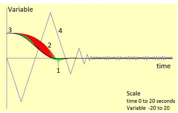
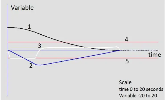
Figure 3.1: 1968 Fast Model Predictive Control Strategy Curves:- 1: Predictions with full positive drive, 2: Predictions with full negative drive, 3: Position x, 4: 10*Acceleration (a)

In this simulation, the green (lighter) and red (darker) traces are the predictions with full positive and full negative drive respectively. The curve-4 shows the acceleration. The values of acceleration are plotted with a coefficient of 10 for better visibility. The curve-3 (mostly through the traces) shows the actual path taken by the plant. The simulation shows slight overshoot near the arrowhead of 1, but the system is stable otherwise.

3.2.2

1987 Fast Model Control Strategy

The strategy proposed by Billingsley (1987) in 1987 can be outlined as follows and note that it does not use switches,

Step 1: Set the model states corresponding to the plant state.

Step 2: Run the model with full positive drive. Note the value of model time at which the model acceleration or velocity have negative sign. Record the model position at this instant.

(43)

3.3 New Iterative Fast Model Control Strategy 24

Step 4: Whichever value of offside time is greater apply drive opposite to the corresponding position. Restart the cycle.

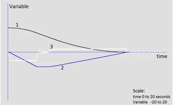
The Simulation of the strategy with the same steplength for model and plant as 0.01 and the initial conditions as positionx= 10, velocityv = 0 and acceleration a= 0 is shown in Fig. 3.2.

Figure 3.2: 1987 Fast Model Predictive Control Strategy Curves:- 1: Predictions with full positive drive, 2: Predictions with full negative drive, 3: Position x, 4: 10*Acceleration (a)

A small overshoot can be seen in Fig. 3.2 as well, near the arrowhead of 2. The simulation results show that the performance of both 1968 (Fig. 3.1) and 1987 (Fig.3.2) fast model control strategies is similar.

3.3

New Iterative Fast Model Control Strategy

In the new Iterative Fast Model Control strategy, the model is considered to be offside if any of the states have a sign different from that of the input. An algorithm of the new strategy can be outlined as follows:

Step 1: Set the system model to the plant state

Step 2: Run the model with full positive drive. Note the time t+ when all the

(44)

3.4 Time Optimality Test 25

Step 3: Reset the system model to the plant state

Step 4: Run the model with full negative drive. Note the time t₋ when all the model states come onside.

Step 5: Compare the times t+ and t− and whichever is greater apply the

corre-sponding drive to the system. Go to Step 1

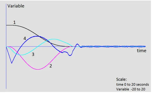
The simulation of the strategy is shown in Fig. 3.3, again the model/plant steplength and initial conditions are same as before, position x = 10, velocity v = 0 and acceleration a= 0.

Figure 3.3: Iterative Fast Model Control Strategy Curves:- 1: Predictions with full positive drive, 2: Predictions with full negative drive, 3: Positionx, 4: 10*Acceleration (a)

Fig. 3.3 shows that there is no overshoot in the system response. In this simu-lation, curve-1 and curve-2 indicate that the new Iterative Fast Model Control strategy is cautious and hence will deliver more stable and less oscillatory per-formance than its predecessors.

3.4

Time Optimality Test

Time optimal control is desirable for many control systems. Fast Model Control can be used to achieve near time optimal control performance. According to Pontryagin et al. (1963) if the input to an nth _{order system is switched} _n

(45)

To assess the degree of time optimality of the Iterative Fast Model Control, the system is taken backwards in time to a certain location noting the time tbk and

then the Iterative fast model control algorithm is used to bring it back to home noting the time of travel tret. The comparison of tbk and tret would verify the

time optimality of the algorithm.

A third order cascaded integrator system is considered to assess the performance of the Iterative Fast Model Control strategy. The initial values of the states of the system are considered as zero.

Then the system is taken backwards in time for 5 seconds. The input is switched two times between full positive drive and full negative drive to reach to a desti-nation, then the values of the new destination states are noted. Taking these new values as initial conditions the system is then run with the new Iterative Fast Model Control Strategy to return to the initial starting position.

The system can be modelled as d3

x

dt3 =u where u = ±1. As this is a third order

system, the input is switched twice att1 = 1 andt2 = 3 while going backwards in

time. At the new destination, the initial conditions for the strategy are found as position x = ₋12.337451, velocity v = 4.5551 and acceleration a = ₋1.010001. The steplengths for model and plant are considered same, 0.01. The simulation of the system is shown in (Fig.3.4).

(46)

The curve-5 in Fig. 3.4 shows the backward journey of acceleration a and the curve-4 show the journey of acceleration a with Iterative Fast Model Control. The backward journey of position x is hidden behind the predictions with full positive and full negative drive. Curve-3 shows the path taken by position x to return to initial starting point.

From Fig.3.4 it can be observed that the strategy takes approximately just over (1

3)

rd _{of 20 i.e. 7 seconds to return to starting point or home. The resulting}

ratio of travel-to-starting-point timetret against the optimal time of 5 sec i.e. tbk

appears to be around 1.4. A more vigorous time optimality test is carried out ahead.

As seen in the simulation, the acceleration enters a limit cycle or dithers, after system reaches initial starting point. Due to the quantization effects, the system will never reach to the exact starting point, hence resulting in dithering.

A less precise arrival at the origin can however be the decided by redetermining the error window around the starting point or home. The error for verifying arrival at the starting point can be calculated as follows,

error =x2 + ˙x2+ ¨x2 (3.1)

and the condition such as error _≤ 0.0001 will allow the system to settle down at certain states. This will leave a small window of error defined by the error condition where states will be very near to 0 but not at exact 0.

When the system or plant enters in this window it will be considered to have ‘arrived’ at home. The error can be calculated by any method but it is the ‘error condition’ that determines the arrival at home. It will be shown ahead that the error condition can be reduced up to a value of 10−10_.

(47)

Figure 3.5: Iterative Fast Model Control with Third Order System, termination using error condition. Curves:- 1: Predictions with full positive drive, 2: Predictions with full negative drive, 3: Positionx, 4: 10*Acceleration (a), 5: 10*Backward journey of acceleration (a) fromx= 0,v= 0 anda= 0

Fig. 3.5 shows the termination upon arrival at home. The final values of the individual variables are found as x=₋0.000246, v = 0.0026 and a= 3_×10−16_.

The time optimality ratio is found to be 1.5. The time optimality test is then performed on a greater scale to evaluate the performance of Iterative Fast Model Control. Its performance is then compared with the performance of previous fast model control strategies.

The test is carried out by considering all possible combinations of switching times between 0 and 5 seconds at intervals of 0.1 seconds to go backwards. For example (t1 = 1 andt2 = 3) or (t1 = 0.1 andt2 = 1.2) etc. The measure of time optimality

is the ratio of, time taken to return to initial starting position and the backward travel time (5 seconds).

The system is considered as ‘arrived to initial position’ when the error condition is satisfied. The simulations for all three strategies (1968, 1987 and IFMC) are carried out. The resulting values are plotted as a colour point with switching timest1 and t2. t1 values (0 to 5 step 0.1) are along x-axis andt2 (0 to 5 step 0.1)

(48)

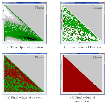
3.5 Simulation Results and Analysis 29

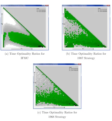
(a) Time Optimality Ratios for IFMC

(b) Time Optimality Ratios for 1987 Strategy

[image:48.595.125.507.90.502.2]

(c) Time Optimality Ratios for 1968 Strategy

Figure 3.6: Color Plots of Time Optimality Ratios

In the Fig. 3.6a, Fig. 3.6b and Fig. 3.6c inside the triangle the darkest (Black) points show the ratios below one. The darker (Green) points show the ratios between 1 and 1.5. The Gray points show the ratios between 1.5 and 2. The White points show the ratios over 2.

3.5

Simulation Results and Analysis

(49)

3.5 Simulation Results and Analysis 30

of white areas) Fig. 3.6a. It is because in IFMC strategy all three variables are considered to be onside before making a decision on, which drive to apply whereas in 1987 and 1968 strategies only two variables are considered.

Thus, IFMC strategy gives more cautious control. Hence, in case of a fourth or higher order systems, IFMC strategy is likely to give more stable performance than 1987 strategy. The time optimal performance of 1968 strategy is inferior to 1987 strategy hence it is not considered for a fourth order system.

A comparison of Fig. 3.7 with Fig. 3.8 shows that for a fourth order system the new Iterative Fast Model Control strategy gives a more stable performance than the 1987 strategy in which switching times are in a converging geometric series.

(50)

3.6 Accuracy in achieving target 31

Figure 3.8: Iterative Fast Model Control - Fourth Order System Curves:- 1: Predictions with full positive drive, 2: Predictions with full negative drive, 3: Position x, 4: 10*Jerk (j)

3.6

Accuracy in achieving target

Along with the time optimality of the strategy, it will be of interest to assess the performance of the strategy in terms of reaching the position of the starting point. As the position is derived from the velocity and the velocity is derived from the acceleration that receives the input, it is important to get the position nearest to the settling point’s position (here-on target) first. The colour plots for position from all three strategies are shown in Fig.3.9.

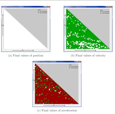
In these plots, the darker gray (red) points represent values between 0.001 and 0.0001, the lighter gray(green) points represent values between 0.0001 and 0.000001. The white points show the values that are less than 0.000001 or even smaller which can be considered as 0. It can be clearly seen that the IFMC strategy gets much closer to the target value than the other strategies.

The proximity to the target position is influenced by the steplength and the error condition. In this case, the target position isx= 0, and the two large white areas in the Fig. 3.9a show state values for position that are zero. It also shows that many values are above the limit.

(51)

(a) Final values of position for IFMC Strategy

(b) Final values of position for 1987 Strategy

[image:51.595.127.509.83.493.2]

(c) Final values of position for 1968 Strategy

Figure 3.9: Final values of State (position) for different strategies

to the top, it becomes necessary to reduce the step-length as the distance to the top becomes smaller and smaller.

Similarly, if the steplength of the plant is reduced as the target gets closer and closer, it is possible to get near optimum proximity to the target. The exact target values will never be reached due to the quantization effects. Thus, the steplength for the plant is reduced by dividing ‘the time taken by the model to come onside’ by 1000 as the target is approached.

(52)

(a) Time Optimality Ratios (b) Final values of position

Figure 3.10: Color Plots IFMC Strategy with Smaller Steplength

In the simulations so far, theerror _≤0.0001 is used as the terminating condition. For the conditions whereerror _≤(0.00001orless), it is found that the acceleration enters a limit cycle or dithers. Another option is to calculate the error in such a way that terminating conditions at a smaller level can be used. One way is to calculate error is shown in3.2.

error=x2+ ˙x2dt2+ ¨x2dt4 where dt= 0.01 (3.2)

The idea of multiplying the squares of variables bydt′_s _{is that if started from the}

origin, acceleration is checked after time dtthen the velocity would be vdt2 and the position would be xdt3. Thus, it would be fair to confirm arrival at target if final values of state - position xare less than 10−6_.

Hence, to terminate upon arrival at starting point, the error needs to be compared with a very small number such as 10−10_{. When this error is compared as}_error_≤

0.0000000001 in the IFMC strategy, the final values for all the states are found as in Fig. 3.11.

In these figures as well, the white points (region) indicate values less than 10−6_,

the light gray (green) points indicate values between 10−4 _{and 10}−3_{, the darker}

gray (red) points indicate values between 10−3 _{and 10}−2 _{and the black points}

(53)

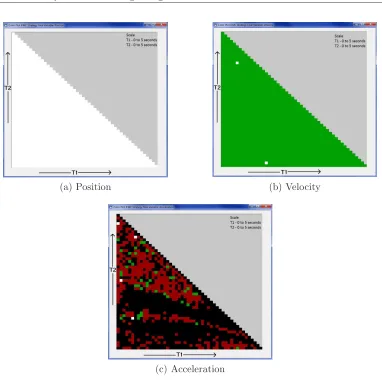
(a) Position (b) Velocity

[image:53.595.130.512.84.465.2]

(c) Acceleration

Figure 3.11: Color Plots of Final Variable Values

When (Fig.3.11a)is compared with (Fig.3.9a), it showed the significant improve-ment in the results with all the values being less than 10−6_.

Fig. 3.11b shows that the most of the values for velocity are less than 10−4 _but

greater than 10−6_{. For acceleration (Fig.} _3.11c_{) shows that many values are over}

10−2 _{and very few less than 10}−6_{. Thus, to improve the results in terms of final}

values of velocity and acceleration, the error is calculated

Analysis and development of iterative fast model control strategies for systems with constraints

University of Southern Queensland

Certification of Dissertation

ENDORSEMENT

Acknowledgments

Contents

List of Figures

Notations and Definitions

Chapter 1

Background

Motivation and Hypothesis

Research Objectives

Structure of the Thesis

Chapter 2

Existing control Strategies

Control methods: Unconstrained design philosophies

Control methods with input/state constraints

Control of Cascaded Integrator Systems

Lyapunov Stability

Evolution of Fast Model Control Strategies

Conclusion

Introduction

Previous Fast Model Control Strategies

1987 Fast Model Control Strategy

New Iterative Fast Model Control Strategy

Time Optimality Test

Simulation Results and Analysis

Accuracy in achieving target