RIT Scholar Works
Theses
8-2019
Deep Grassmann Manifold Optimization for
Computer Vision
Breton Lawrence Minnehan
Breton Lawrence Minnehan
A dissertation submitted in partial fulfillment of the requirements for the degree of
Doctor of Philosophy
in Engineering
Kate Gleason College of Engineering Rochester Institute of Technology
August 2019
Signature of the Author
Certified by
ROCHESTER INSTITUTE OF TECHNOLOGY ROCHESTER, NEW YORK
CERTIFICATE OF APPROVAL
Ph.D. DEGREE DISSERTATION
The Ph.D. degree dissertation of Breton Lawrence Minnehan has been examined and approved by the
dissertation committee as satisfactory for the dissertation required for the
Ph.D. degree in Engineering
Dr. Andreas Savakis, Dissertation Advisor Date
Dr. Christopher Kanan, Committee Member Date
Dr. Andres Kwasinski, Committee Member Date
Dr. Panos P. Markopoulos, Committee Member Date
by
Breton Lawrence Minnehan Submitted to the
Kate Gleason College of Engineering Ph.D. in Engineering Program in partial fulfillment of the requirements for the
Doctor of Philosophy Degree
at the Rochester Institute of Technology
Technical Abstract
In this work, we propose methods that advance four areas in the field of computer vision: dimensionality reduction, deep feature embeddings, visual domain adaptation, and deep neural network compression. We combine concepts from the fields of manifold geometry and deep learning to develop cutting edge methods in each of these areas. Each of the methods proposed in this work achieves state-of-the-art results in our experiments. We propose the Proxy Matrix Optimization (PMO) method for optimization over orthogonal matrix manifolds, such as the Grassmann manifold. This optimization technique is designed to be highly flexible enabling it to be leveraged in many situations where traditional manifold optimization methods cannot be used.
We first use PMO in the field of dimensionality reduction, where we propose an iterative optimization approach to Principal Component Analysis (PCA) in a frame-work called Proxy Matrix optimization based PCA (PM-PCA). We also demonstrate how PM-PCA can be used to solve the generalLp-PCA problem, a variant of PCA that uses arbitrary fractional norms, which can be more robust to outliers. We then present Cascaded Projection (CaP), a method which uses tensor compression based on PMO, to reduce the number of filters in deep neural networks. This, in turn, reduces the number of computational operations required to process each image with the network. Cascaded Projection is the first end-to-end trainable method for network compression that uses standard backpropagation to learn the optimal tensor compres-sion. In the area of deep feature embeddings, we introduce Deep Euclidean Feature Representations through Adaptation on the Grassmann manifold (DEFRAG), that leverages PMO. The DEFRAG method improves the feature embeddings learned by deep neural networks through the use of auxiliary loss functions and Grassmann
by
Breton Lawrence Minnehan Submitted to the
Kate Gleason College of Engineering Ph.D. in Engineering Program in partial fulfillment of the requirements for the
Doctor of Philosophy Degree
at the Rochester Institute of Technology
Outreach Abstract
As digital imaging sensors have become ubiquitous in modern society, there has been increasing interest in extracting information from the data the sensors collect. The study of extracting information from visual data is known as computer vision. The field of computer vision has made significant progress in recent years thanks in large part to the emergence of deep learning. In this work, we present novel methods that advance five areas of computer vision and deep learning. The first area of contribution is Grassmann manifold optimization, a constrained optimization technique that has application in many fields, including: physics, communications, deep learning, and computer vision. In the second area of research, we propose methods for dimensionality reduction based on our manifold optimization method. Dimensionality reduction is used in many fields to reduce high dimensional data to a more compact representation. In the third area of research we propose a method for compressing deep neural networks in order to reduce the number of computations required and reduce the processing time. In the fourth area of research we propose a method that encourages deep networks to learn better representations of data by grouping similar classes closer than dissimilar classes. The fifth area of research is in the field of domain adaptation, that aims to solve a problem known as domain shift encountered due to the difference between the data that a classifier is trained on and data the classifier encounters when deployed. The domain adaptation method developed in this work mitigates the domain shift by finding correspondences between the data in two domains and uses the correspondences to transfer the labels from the labeled source samples to the unlabeled target samples. Our proposed work in each of these areas has many applications such as pedestrian detection in autonomous vehicles, classifying remote sensing images and object recognition on mobile devices.
1 Introduction 1
1.1 Contributions . . . 3
2 Deep Learning 5 2.1 Artificial Neural Networks . . . 5
3 Manifold Optimization 13 3.1 Mathematical Definitions . . . 13
3.2 Manifold Operations . . . 16
3.3 Proposed Proxy Matrix Manifold Optimization . . . 18
3.3.1 One-Step iterative manifold optimization . . . 18
3.3.2 Two-step iterative manifold optimization . . . 20
3.3.3 Proxy Matrix Optimization . . . 22
3.4 Experimental Results . . . 26
3.4.1 Learning Rate Convergence Analysis . . . 26
3.4.2 Number of Iterations for Convergence . . . 29
3.5 Implementation Details . . . 32
4 Dimensonality Reduction 33 4.1 Background . . . 33
4.1.1 Grassmann Optimization for Linear Dimensionality Reduction 34 4.1.2 L2-norm Based PCA . . . 35
4.1.3 L1-norm Based PCA Background . . . 36
4.1.4 Lp-Norm Based PCA . . . 37
4.1.5 Linear Discriminant Analysis . . . 37
4.2 Dimensionality Reduction Using Proxy-Matrix Optimization . . . . 38
4.2.1 Lp-PCA . . . 39
4.2.2 Weighted Contribution PCA . . . 40
4.3 Experiments . . . 41
4.3.1 Initialization Experiments . . . 43
4.3.2 L2-PCA Experiments . . . 44
4.3.3 L1-PCA Experiments . . . 45
4.3.4 Lp-PCA Experiments . . . 50
4.3.5 Weighted Contribution PCA Experiments . . . 54
4.3.6 Labeled Faces in the Wild Outlier Experiments . . . 57
4.3.7 Labeled Faces in the Wild Occlusion Experiments . . . 63
4.4 Remarks . . . 68
5 Cascaded Projection Network Compression 69 5.1 Introduction . . . 70
5.2 Related Work . . . 72
5.3 Cascaded Projection Methodology . . . 73
5.3.1 Problem Definition . . . 73
5.3.2 Single Layer Projection Compression . . . 74
5.3.3 Cascaded Projection Compression . . . 75
5.3.4 Mixture Loss . . . 77
5.3.5 Compressing Multi-Branch Networks . . . 77
5.3.6 Back-Propagated Projection Optimization . . . 79
5.4 Experiments . . . 80
5.4.1 Layer-wise Experiments . . . 81
5.4.2 CaP Ablation Experiments . . . 82
5.4.3 ResNet Compression on CIFAR 10 . . . 85
5.4.4 VGG16 Compression with ImageNet . . . 85
5.5 Observations . . . 87
6 Feature Embedding 88 6.1 Feature Embedding Background . . . 88
6.2 Learning Deep Feature Embeddings on Euclidean manifolds . . . 91
6.2.1 Clustering Auxiliary Loss . . . 92
6.2.2 Grassmann manifold Retraction . . . 92
6.3 Feature Learning Experiments . . . 92
6.3.2 Qualitative MNIST Experiments . . . 95
6.4 Remarks . . . 96
7 Domain Adaptation 97 7.1 Domain Adaptation Background . . . 98
7.1.1 Deep domain adaptation . . . 101
7.2 Domain Adaptation Proposed Work . . . 103
7.2.1 Center-loss feature training . . . 104
7.2.2 Adaptive Batch Normalization . . . 105
7.2.3 Subspace Alignment on the LPP manifold . . . 106
7.2.4 Feature Clustering using Gaussian Mixture Model . . . 108
7.2.5 Dual-Classifier Pseudo-Label Filtering . . . 109
7.2.6 Label Transfer via manifold clustering . . . 110
7.3 Domain Adaptation Experiments . . . 112
7.3.1 Network Architecture . . . 112
7.3.2 Digit Classification . . . 114
7.3.3 Remote Sensing Datasets . . . 118
7.4 Remarks . . . 119
List of Figures
2.1 Visual depiction of the Perceptron. . . 6 2.2 Visual depiction of using multiple perceptrons to generate multiple
outputs for a single input. . . 7 2.3 Visual depiction of a Multiple Layer Perceptron (MLP). . . 8 2.4 Visual depiction of a single layer of a Convolutional Neural Network
(CNN). . . 9 2.5 Visual depiction of the decomposition of a convolution operation into
a locally connected implementation. . . 10 2.6 ResNet convolutional network architecture. . . 11 2.7 Densely connected convolutional network architecture. . . 12
3.1 Visual depiction of the One-Step retraction process. The point is first updated based on the gradients calculated through backpropagation. Then the point is retracted directly to the closest point on the manifold. This process is repeated until some stopping criteria is met. . . 19 3.2 Visual depiction of the Two-Step retraction process. The point is first
updated based on the gradients calculated through backpropagation. Then the point is first projected to the tangent-space (green plane) at Riusing Equation (3.2), the projection is shown as the dotted blue
line. Then the point is retracted from the tangent space to the closest point on the manifold using Equation (3.3). This process is repeated until some stopping criteria is met. . . 21
3.3 Visual depiction of the Proxy Matrix Optimization process. The proxy matrix,Pi, is first retracted to the manifold using Equation (3.3). Then the gradients∇R(Pi)in ambient space, to move the proxy matrix in a direction that minimize the loss of its retraction. These gradients are used to move the proxy matrix in Euclidean space in the direction that minimizes the loss. . . 24 3.4 Example behavior of the loss when varying the learning rate using the
Two-Step retraction method. The learning rates used were: Red 10.0, Blue 1.0, Green 0.1, Black 0.01. . . 28 3.5 Example behavior of the loss when varying the learning rate using
the Proxy-Matrix method. The learning rate was reduced by an order of magnitude at 50% and again at 75% through training.The learning rates used were: Red 1000.0, Blue 100.0, Green 10.0, Black 1.0. . . 29 3.6 Convergence plot of Two-Step and Proxy Matrix methods, Blue and
Red plots respectively, forL2-PCA. . . 30 3.7 Convergence plot of Two-Step and Proxy Matrix methods, Blue and
Red plots respectively, forL1-PCA. (Note the horizontal axis is in log-scale.) . . . 31 3.8 Convergence plot of Two-Step and Proxy Matrix methods, Blue and
Red plots respectively, forL0.5-PCA. (Note the horizontal axis is in log-scale.) . . . 31
4.1 Relative percent reduction in error for 5 random initializations vs. initializing with theL2 solution. Experiments were run on 10 sets of data with four different dimensionality reduction objectives. . . 43 4.2 Average reprojection error for standard SVD basedL2-PCA and
pro-posed PM-L2-PCA methods for varying number of principal compo-nents. . . 45 4.3 Average reprojection error for four PCA methods for varying number
of principal components. The mean from runs on 10 separate dataset are plot. The results fromL2-PCA are shown in blue, BF-L1-PC are shown in green, PCA-RPR are shown in red, and PM-L1-PCA-PRJ are shown in cyan. . . 46 4.4 Percent improvement of the PMO and Bit-FlippingL1-PCA
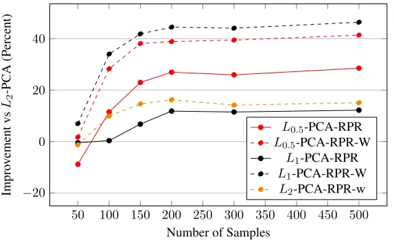
4.5 Percent improvement of the PMO and Bit-FlippingL1-PCA methods relative toL2-PCA for datasets with various number of samples. Mean calculated based on 10 runs on randomly initialized datasets. . . 48 4.6 Processing time forL1-PCA algorithms run on 500 samples from the
toy datasets with varying number of principal components. . . 49 4.7 Processing time forL1-PCA algorithms run on varying number of
samples 50-500 from the toy calculating 10 principal components. . 50 4.8 Improvement in reprojection error using the reprojection objective
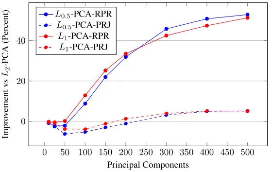
with the PM-Lp-PCA framework for different number of components, all relative toL2-PCA. . . 52 4.9 Improvement in reprojection error using the projection objective with
the PM-Lp-PCA framework for different number of components, all relative toL2-PCA. . . 52 4.10 Improvement in reprojection error using the reprojection objective
with the PM-Lp-PCA framework for different dataset sizes, all relative toL2-PCA. . . 53 4.11 Improvement in reprojection error using the projection objective with
the PM-Lp-PCA framework for different dataset sizes, all relative to L2-PCA. . . 53 4.12 Improvement in reprojection error using the reprojection objective
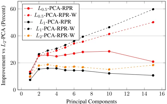
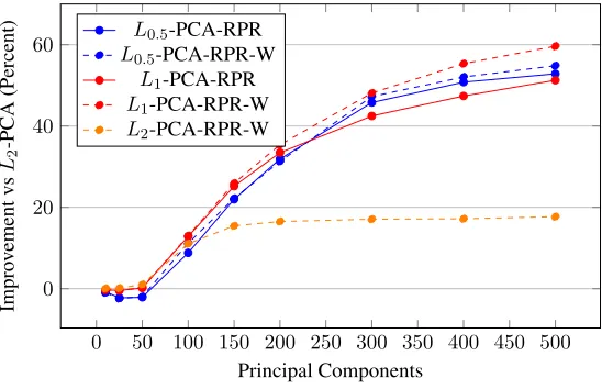
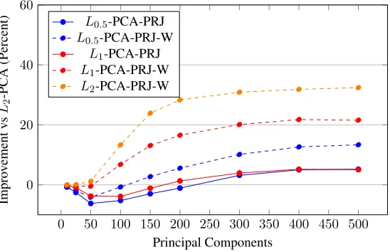
with the PM-Lp-PCA framework usingpof 0.5, 1.0, 2.0. both without and with weighted-contributions, solid and dashed lines respectively. All results are relative improvement toL2-PCA. . . 55 4.13 Improvement in reprojection error using the projection objective with
the PM-Lp-PCA framework usingpof 0.5, 1.0, 2.0. both without and with weighted-contributions, solid and dashed lines respectively. All results are relative improvement toL2-PCA. . . 55 4.14 Improvement in reprojection error using the reprojection objective
with the PM-Lp-PCA framework for different dataset sizes, all relative toL2-PCA. . . 56 4.15 Improvement in reprojection error using the projection objective with
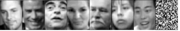
the PM-Lp-PCA framework for different dataset sizes, all relative to L2-PCA. . . 56 4.16 Example images of faces in the Labeled Faces in the Wild Dataset.
4.17 Improvement in reprojection error for the LFW dataset with varying values ofpusing the proposed PM-Lp-PCA framework, all relative to L2-PCA. . . 58 4.18 Improvement in reprojection error using the reprojection objective
with the PM-Lp-PCA framework, both with and without the weighted loss functions, all relative toL2-PCA. . . 59 4.19 Improvement in reprojection error using the projection objective with
the PM-Lp-PCA framework, both with and without the weighted loss functions, all relative toL2-PCA. . . 60 4.20 Reprojection of face images using the proposed POM-L1-PCA and
standardL2-PCA principal components extracted from corrupted face training set. First row: Input Image. Second row: Reprojection using L2-PCA. Third row: Reprojection using PM-L1-PCA with projection formulation. Third row: Reprojection using PM-L1-PCA with repro-jection formulation. Fourth row: Reprorepro-jection using PM-L1-PCA with reprojection formulation and weighted contribution. Fifth row: Reprojection using PM-L1-PCA-W with Projection Maximization Formulation. . . 61 4.21 Example principal components resulting from training different PCA
methods on a dataset of facial images with 10% of the image corrupted with uniform noise. The rows are organized as follows. First row: L2-PCA. Second row: projection formulation of PM-L1-L2-PCA. Third row: reprojection formulation of PM-L1-PCA. Forth row: reprojection formulation of PM-L1-PCA with weighted contribution. . . 62 4.22 Improvement in reprojection error using the reprojection objective
with the PM-Lp-PCA framework, both with and without the weighted loss functions, all relative toL2-PCA. . . 64 4.23 Improvement in reprojection error using the projection objective with
4.24 Example principal components resulting from training different PCA methods on a dataset of facial images with all images corrupted by a patch covering 10% to 30% of the image made of uniform noise. The rows are organized as follows. First row: L2-PCA. Second row: projection formulation of PM-L1-PCA. Third row: reprojection formulation of PM-L1-PCA. Fourth row: reprojection formulation of PM-L1-PCA with weighted contribution. . . 65 4.25 Reprojection of face images using the proposed PM-L1-PCA and
standardL2-PCA principal components extracted from the corrupted face training set. First row: Input Image. Second row: Reprojection using L2-PCA. Third row: Reprojection using PM-L1-PCA with Reprojection Minimization Formulation. Fourth: Reprojection using PM-L1-PCA with Projection Maximization Formulation. Fifth row: Reprojection using PM-L1-PCA-W with Projection Maximization Formulation. . . 66 4.26 Reprojection of face images using the proposed PM-L1-PCA and
standardL2-PCA principal components extracted from the corrupted face training set. First row: Input Image. Second row: Reprojection usingL2-PCA. Third row: Reprojection using PM-L1-PCA with Re-projection Minimization Formulation. Fourth row: ReRe-projection using PM-L1-PCA with Projection Maximization Formulation. Fifth row: Reprojection using PM-L1-PCA-W with Projection Maximization Formulation. . . 67
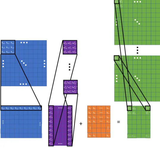
5.1 Visual representation of network compression methods on a single CNN layer. Top row: Factorization compression with a reprojection step that increases memory. Middle row: Pruning compression where individual filters are removed. Bottom row: Proposed CaP method which forms linear combinations of the filters without requiring repro-jection. . . 71 5.2 Visual representation of the compression of a CNN layer using the CaP
method to compress the filtersWiandWi+1in the current and next
layers using projectionsPiandPTi respectively. The reconstruction
5.3 Illustration of simultaneous optimization of the projections for each layer of the ResNet18 network using a mixture loss that includes the classification loss and the reconstruction losses in each layer for intermediate supervision. We do not alter the structure of the residual block outputs, therefore we do not affect residual connections and we do not compress the outputs of the last convolution layers in each residual block. . . 78 5.4 Plot of the reconstruction error (vertical axis) for the range of
com-pression (left axis) for each layer of the network (right axis). The reconstruction error is lower when early layers are compressed. . . . 81 5.5 Plot of the classification accuracy (vertical axis) for the range of
compression (left axis) for each layer of the network (right axis). The classification accuracy remains unaffected for large amounts of compression in a single layer anywhere in the network. . . 81 5.6 Classification accuracy drop on CIFAR10, relative to baseline, of
compression methods (CaP, PCAS [155], PFEC [85] and LPF [60]) for a range of compression levels on ResNet18 (Right) and ResNet50 (Left). . . 83
6.1 Example images from MNIST (top row) and Fashion MNIST (bottom row). . . 93 6.2 Visualization of feature representations in 2D trained on the MNIST
dataset using a combination of Classification Loss and Auxiliary Loss. Features are learned using (a) Softplus activation from classification loss only; (b) linear activation function; (c) center loss [150]; (d) contrastive center loss [111]; (e) our DEFRAG method. . . 95
7.1 Overview unsupervised domain adaptation of deep network to the target domain. Adaptive batch normalization is used for training and adaptation in both source and target domains. Subspace alignment is performed for source and target features on the LPP manifold and the features are clustered to determine if label transfer is appropriate based on a clustering criterion. Label transfer is performed by assigning labels from the closest source cluster to each target cluster and using them to retrain the network. . . 103 7.2 Sample images from different datasets showing variations in the same
7.3 Feature visualization using t-SNE plots. The two leftmost columns show the Source (Red) and Target (Blue) features though each stage of the MALT-DA pipeline. The first column (Left) shows the source and target features, red and blue respectively, resulting from the un-adapted network with ABN. The second column depicts the same features after our Subspace Alignment process on the LPP manifold. The third column shows the only the features from the target domain that passed the dual-classifier pseudo label filtering, the different colors correspond to the class of each data-point. The last column displays the visualization of the, unfiltered, features resulting from the proposed network adaptation method.. Each row corresponds to a different adaptation problem. First: from MNIST to USPS dataset. Second: from MNIST to the SVHN dataset. Third: from Syn. Digits to the SVHN dataset. Last: from USPS the MNIST dataset. . . 117 7.4 Sample images from the shared classes in the UCM (top row) and
4.1 Improvement reprojection errors, relative toL2-PCA, for clean test set when PM-Lp-PCA with varying values ofpis trained on corrupted Synthetic-Dataset. . . 51
5.1 Network compression ablation study of the CaP method compress-ing the ResNet18 Network trained on the CIFAR100 dataset. (Bold numbers are best). . . 82 5.2 Comparison of CaP with pruning and factorization based methods
using ResNet56 and ResNet110 trained on CIFAR10. FT denotes fine-tuning. (Bold numbers are best). * Only the relative drop in accuracy was reported in [160] without baseline accuracy. . . 84 5.3 Network compression results of pruning and factorization based
meth-ods without fine-tuning. The top-5 accuracy of the baseline VGG16 network varies slightly for each of the methods due to different models and frameworks. (Bold numbers are best). Results marked with * were obtained from [53]. . . 86 5.4 Network compression results of pruning and factorization based
meth-ods with fine-tuning. (Bold numbers are best). . . 86
6.1 Network Architecture . . . 93 6.2 Fashion MNIST Results . . . 94
7.1 Quantitative results for SoftMax and Center-loss networks with 2D feature representations. . . 105 7.2 Accuracy of digit classification datasets. . . 115
The contributions of this dissertation can roughly be separated into four distinct areas: dimensionality reduction, network compression, deep feature embeddings, and visual domain adaptation. However, all four areas are closely related and improvements in one can prove useful in the others. There are two core conceptual threads that tie all of these areas together: deep learning and manifold optimization. Chapter 2 provides the reader with the theoretical background on the former while Chapter 3 focuses on the latter.
Deep Convolutional Neural Networks (CNNs) and their variants have emerged as the architecture of choice for computer vision. Deep networks have achieved state-of-the-art results in object class recognition [73], [130], [48], face recognition [123], semantic segmentation [90], pose estimation [149], and visual tracking [106] among other applications.
There is a large body of work studying Grassmann manifolds and their applications in the field of computer vision. Grassmann manifolds have been used in distance met-ric learning and subspace analysis for problems such as domain adaptation and visual object tracking. In this work we demonstrate how Grassmann manifold optimization can be used to perform robust Principal Component Analysis in a computationally efficient manner. We demonstrate how by restricting fully-connected layers of Artifi-cial Neural Networks we can ensure the feature embedding is a Euclidean space. This provides multiple benefits including that the resulting features can be accurately com-pared using the Euclidean distance. Additionally, we demonstrate how this framework can be adopted to obtain an end-to-end method for visual domain adaptation.
Dimensionality reduction methods have an incredibly vast array of applications
in signal processing, such as signal compression or classification applications in computer vision. Most computer visions tasks require extremely high dimensional data to be reduced to only the pertinent information in the form of features. In this work we propose new methods for dimensionality reduction using iterative optimization methods originally developed in the field of deep learning.
The field of feature embedding has received some attention recently from the standpoint of improving feature clustering [101] or for zero/one-shot learning. In each of these cases, attempts have been made to learn image embeddings using deep neural networks where images of similar subjects/classes have features that are close together and images of different subjects/classes are further apart. However, many of these works ignore a key problem, the feature spaces they learn lack an orthonormal basis, and thus are not Euclidean spaces. Yet these methods continue to use the Euclidean distance as a similarity metric for the feature embeddings. Furthermore, there are many examples of methods which use the features extracted from the last layer of a deep neural network, specifically after a rectified linear activation function, as their feature embedding. This is even more problematic as the feature representation is inherently sparse. We will go into more detail as to why this is a problem in Chapter 6. We will also discuss how Grassmann manifold optimization can be used during the training process to generate proper Euclidean space embeddings such that the resulting features can be accurately compared using the Euclidean metric.
There are many potential applications for learning deep Euclidean embedding spaces from direct use in deep networks to reduce overfitting and improve the clus-tering behavior. For applications where there is only a limited number of samples available, such as person re-identification, a k-Nearest Neighbor (kNN) classifier is typically used which often relies on the Euclidean distance metric between features. In a different context, deep Euclidean embeddings could be used in applications such as visual object tracking.
the target, unless somehow adapted. This adaptation process is known as domain adaptation and is a quickly developing area of research. As is evident from the multiple examples there are many applications that would greatly benefit from advances in domain adaptation. We propose the development of domain adaptation techniques that leverage our work in the two other fields to provide a method that is better suited for the situations commonly faced in modern computer vision applications.
The remainder of this work is organized as follows: Chapter 2 discusses related work and other background knowledge in the field of deep learning. Chapter 3 provides background knowledge on manifold optimization and presents a new method developed in this work. Chapter 4 outlines our work in the field of dimensionality reduction. Chapter 5 applies our manifold optimization method to the field of deep neural network compression for improved efficiency and reduced size. Chapter 6 introduces new methods for learning better features representations though the combination of deep learning and manifold optimization. Chapter 7 presents our work in the field of domain adaptation. Finally, Chapter 8 provides concluding remarks.
1.1
Contributions
The contributions of this dissertation are as follows:
• Develop optimization on Grassmann Manifolds using recent advancements in gradient-based optimization to accelerate convergence and improve robustness to non-convex loss functions. We call our new Grassmann manifold optimization technique Proxy Matrix Optimization.
• Develop a novel dimensionality reduction framework that uses an artificial neural network approach for Grassmann manifold optimization. The proposed framework can solve for various dimensionality reduction techniques through simple changes in the network’s training loss function.
• Develop a new method for compression of deep neural networks using a decom-position method and Proxy Matrix Optimization, that is trained in an end-to-end manner.
Deep learning is one of the fastest growing areas of research in the field of computer science. In recent years there have been countless breakthroughs across a wide array of problem areas that have been achieved through use of deep learning methods. In this chapter we provide a general overview of the field of Artificial Neural Networks (ANNs) and Deep Learning.
2.1
Artificial Neural Networks
The fast-growing field of deep learning traces its origins back to the artificial perceptron [115] first proposed in the 1950’s. The design of the perceptron is said to be inspired by the connections on neurons. Where, similar to a biological neuron, the perceptron’s activation is determined based on a weighted summation of its input.
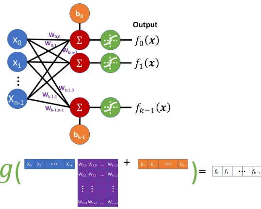
The basic building block of ANNs is the artificial perceptron, shown in Figure 2.1. At its core the perceptron is a weighted summation of an input vector that is passed through a nonlinearity. This operation consists of an inner product of the input vector,x, and the weight vector,w. A bias,bis added to the weighted sum, and then a nonlinear functiong(·)is applied as:
f(x) =g(xTw+b) (2.1)
The perception can easily process multiple inputs simultaneously, known as batch processing. Additionally, perceptrons can be used in parallel to generate what is known as a layer of perceptrons with multiple outputs, as shown in Figure 2.2. This doesn’t
Figure 2.1: Visual depiction of the Perceptron.
require any change to the linear algebra except that the weight vector,w, is replaced with am×nweight matrix, generated by stacking the mdifferentn-dimensional weight vectors wheremis the number of perceptrons (output dimension).
The power of the artificial perceptron becomes more apparent whendlayers of perceptrons are stacked on top of each other, where the output of one layer is used as the input to the next layer, as shown in Figure 2.3. A non-linear function is used as the activation function for each perceptron. Again, the mathematics for the Multi-Layer Perceptron (MLP) do not change besides stacking the operations of each perceptron as:
Figure 2.2: Visual depiction of using multiple perceptrons to generate multiple outputs for a single input.
weight connecting the output nodeoj with the nodeoiin the previous layer is given as:
∂L ∂wi,j
=oi(oj−tj)oj(1−oj) (2.3)
wheretjis the ground truth output value for the nodeoj. If the nodeojis not an output node the partial derivative of the loss function with respect to the weight connecting it to the nodeoi in the previous layer is∂w∂Li,j =oiδjwhereδjis given as:
δj = (
X
l∈L
wi,lδl)oj(1−oj) (2.4)
The loss produced by the perceptron for each input is used to update the weight and bias vectors.
Figure 2.3: Visual depiction of a Multiple Layer Perceptron (MLP).
train deep networks on large datasets. Third, ANNs were viewed as theoretical black boxes with little intuition or framework.
Convolutional Neural Networks [82] were revolutionary because they provided a way for ANNs leverage the spatial information available in imagery. Another benefit to CNNs over MLPs is that they required a much smaller set of trained-parameters. With traditional fully-connected MLPs the number of parameters for each layer was nm wherenis the input dimension (h×w) of the image andm is the number of outputs for the layer is the number of outputs for the layer. For example, a two layer layer fully-connected network with 2516 hidden nodes and 10 output nodes and an input image of size (28×28), requires 203,530 parameters. However, with CNNs the number of parameters for each layer is reduced tomk2 wherek is the size of the convolution kernel, usual 3 to 7 pixels. Therefor a similar convolutional network with(3×3)kernels would require just 33,280 parameters, assuming a global pooling layer is on the last layer to reduce each feature map to a scalar value, as is commonly done. A visual representation of a CNN is given in Figure 2.4. The mathematical formulation for each layer of a CNN is given as:
f(X) =g(XW+b) (2.5)
Figure 2.4: Visual depiction of a single layer of a Convolutional Neural Network (CNN).
∗is the convolution operation. This can be extended for cases where the input has multiple channels by performing the 2D convolution on theH×W ×Cinput with a k×k×Ckernel.
Although it is more efficient to implement a CNN using convolution operations it is important to recognize that this operation can be performed using the MLP formulation. The only change required is that the input image must be decomposed into separate k×kblocks that are vectorized from an input matrixXthat has dimensionsW H×k2. A visual example of this decomposition method is given in Figure 2.5.
The field of deep learning did not fully take off until AlexNet [73] which demon-strated the ability of deep CNNs to classify a large number of classes in ImageNet by leveraging their parallel nature and using Graphic Processing Units (GPUs) during training. The advances in the field of deep learning are too numerous to review here. However, we will outline some of the particular advances that are specifically pertinent to this work.
Figure 2.5: Visual depiction of the decomposition of a convolution operation into a locally connected implementation.
calculated as follows:
¯
xi =
1
T
X
i=(0,T)
xi (2.6)
σ2i = 1
T
X
i=(0,T)
(xi−x¯i)2 (2.7)
ˆ
xi=
(xi−x¯i)
q
σ2 i
(2.8)
the gradients for each update set are better suited for training, especially in early epochs with randomly initialized weights. Batch Normalization allows for much faster training with higher learning rates. Traditionally the statistics and scale/shift values for the activations are learned at training time and frozen at test time, meaning that the activations are whitened based on the statistics of the training set, but not the test set. Another technique that is commonly used to train deep neural networks is dropout [133]. The aim of dropout is to prevent deep networks from overfitting by forcing redundancy into the network. Dropout forces redundancy by randomly selecting a set of neurons in each layer with a given probability, generally between 25% to 50%, and setting their activations to zero. This forces the network to rely on the remaining features in the layer, and thus builds redundancy into the network. The introduction of dropout into the training process allows deeper networks to be trained with a significantly lower risk of overfitting. Convolutional neural network architectures have made significant advances in recent years. In this section we only highlight three commonly used architectures: VGG [129], Residual Networks (ResNet) [49] and Densely Connected Networks (DenseNet) [57]. There are many others that are used for various applications.
The VGG architecture is a traditional convolutional network architecture that was built with the same design in the original CNNs introduced in [80] and popularized in [73]. The VGG architecture generally has several convolutional layers utilizing 3x3 filters followed by a max pooling layer. These convolutional blocks are repeated until the last convolutional features are vectorized and fed into several fully connected layers. This type of architecture is the fundamental type of CNN, yet it is still commonly used throughout the field of deep learning. A common variation is that most researchers introduce batch normalization layers into the network as well.
Figure 2.6: ResNet convolutional network architecture.
flow. This is done by summing the input to each convolutional layer with its output. A visual example of a ResNet is presented in Figure 2.6
Figure 2.7: Densely connected convolutional network architecture.
Manifolds are used through the field of machine learning for various applications such as: dimensionality reduction [20], invariant subspace learning [144, 145], clustering [16, 148], regularization [59], and many more. Of particular interest to this work are matrix manifolds, the Stiefel manifold and the Grassmann manifold. We develop the Proxy Matrix Optimization (PMO) method which improves the convergence of iterative manifold optimization by reformulating the optimization problem to directly incorporate the manifold retraction into the gradient calculation. This reformulation alleviates the constraint on update step size required by previous methods due to their reliance on the tangent space.
In this chapter, we first provide the reader with the definitions of several important manifold structures. We then outline operations that can be performed on specific manifolds. After providing the theoretical background and a review of previous works in the field of manifold optimization, we propose our PMO method for optimizing over the Stiefel and Grassmann manifold. Manifold optimization methods form the core of three out of the four areas of application in this work: dimensionality reduction, improving learned feature embeddings, and network compression.
3.1
Mathematical Definitions
Prior to discussing the field of manifold optimization and our specific contributions, we provide a review of some of the core theory. The works of [2] and [9] provide a more detailed theoretical background on the field of optimization over matrix manifolds. We start with the question: what are manifolds and how are they used? Ad-dimensional
manifold is a setM that is fully covered by a set of charts that form one to one correspondences between points in the setMand elements in thed-dimensional real spaceRd. A more formal definition is supplied in [2]. A manifoldMis a set in a
couple(M,A+)whereA+is a maximal atlas of the setMinto thed-dimensional real spaceRd. An atlasAis a set of charts,(Ua, ϕa), that cover the entire manifold,
S
aUa =M, and overlap smoothly for any pointx∈ Ua∩ Ub. A chart(U, ϕ)is a bijection, one-to-one mapping, of the each of the points in the setU ∈ Mto points in thed-dimensional real spaceRd. Given a chart(U, ϕ)and a pointx∈ U, the bijection
ofϕ(x)maps the point to a coordinate in the real space,ϕ(x)∈Rd. The manifoldM is a smooth manifold if all charts in its atlas are infinitely differentiable over its own set. This is why the atlas is sometimes referred to as the differentiable structure ofM. A d-dimensional vector space ¯v with basis (v1, v2, ...vd) for i ∈ [1, ...d]is a manifold. The manifold structure of¯vis given by the fact that a chartϕexists for the set such that all points in¯vare mapped toRd. This is most easily defined based
on the inverse of mappingϕ−1 =x=Pd
i=1xivi. The manifolds formed by linear subspaces are a special type of manifold, called a linear manifold.
It can be shown that the set of real valued matricesRm×pform amp-dimensional
manifold, as the column vector of the matrix are the basis for the vector spaceε. A chart for this manifold that maps fromRm×ptoRmpis defined as the vectorization
of the matrix, i.e. stacking each of themcolumns of lengthpto form a single vector of lengthmp. This manifold of real-valued matrices is an important manifold for this work as it forms the set on which other submanifolds are defined. Another important property of the real matrix manifold is that it forms a Euclidean space with the traditional inner product given ashX,Yi = ϕ(X)Tϕ(Y). This inner product can also be calculated using the trace of the transposed matrix multiplication as
hX,Yi = tr(XTY). This inner product induces the traditional Frobenious norm
kXk2
F = tr(XTX). For the remainder of this work the manifold of real valued matrices is implied whenever we refer to the matrix manifold.
There are two categories of sub-manifolds of the real matrix manifold that are pertinent to this work: embedded manifolds and quotient manifolds. Embedded matrix manifolds are formulated as the subset of a set of real(m×p)matrices,Rm×p, where
1≤p≤n, and the matrices satisfy an explicit constraint. An example of an embedded manifold in theRm×1, is the unit sphereSm−1, which contains all column vectors
with unit norm i.e. ifX∈Sm−1thenXTX= 1.
manifold is the set of orthogonalp-dimensional subspaces in Rm, this is known
as the Grassmann manifold [44], denoted asGm×p. The Grassmann manifold will be discussed in more detail later in this section. However, the important takeaway here is that if an(m×p)matrixXexists on the Grassmann manifoldGm×p, then any matrix resulting from the right multiplication by an orthonormal(p×p)matrix Q∈ Op×p, exists on the same point in the Grassmann manifold. These are equivalent representations of the point on the Grassmann manifold. It is important to highlight the fact that because quotient manifolds represent equivalence classes, there is not an inherent singular matrix representation of each point on the manifold. Instead, any arbitrary matrix belonging to the given subspace on the manifold can be used to represent the point on the manifold. The results of matrix algebra operations performed on the representative matrix are equivalent regardless of which matrix was selected to represent the subspace.
The first important submanifold of the matrix manifold is the Orthogonal matrix manifold. The Orthogonal manifoldOm×mis formed by the subset of realm×m matrices that satisfy the QTQ = Im. The matrices that make up Om×m have independent columns with unit norms.
Another important manifold is the Stiefel manifold,Sm×p. The Stiefel manifold is an embedded submanifold in the matrix manifoldRm×p where all points on the
manifold,X∈ Sm×psatisfyXTX=I
p. Using this definition the Stiefel manifold is defined as an embedded submanifold in the matrix manifold which is itself an embed-ded manifold inmp-dimensional Euclidean spaceRmp. However, some embedded
manifolds can also be defined in terms of quotient spaces. The benefit to defining a manifold as quotient spaces of well defined manifolds leads to simpler formulae for operations on the manifold. Both StiefelSm×pand Grassmann manifoldsGm×p can be defined as a quotient manifold of the Orthogonal manifoldOm×m. This can be done by representing the set of equivalency classes forSm×p inOm×mas the set[X]
whereX∈ Om×mandQn−p∈ On−p×n−pthen:
[X] =
Ip 0n−p
0p Qn−p
(3.1)
A full derivation of the operations based on the quotient space definition of the Stiefel manifold is provided in [2, 9, 31].
The Grassmann manifoldGm×p is a quotient manifold because it defines a set of equivalence classes, thep-dimensional subspaces inRm. Unlike the Stiefel manifold,
a point on the Grassmann manifold can be be represented as any matrix whose columns span the subspace. Points on the Grassmann manifold are invariant to the ordering of the basis vectors, as long as they span the same subspace. More concretely two
(m×p)matricesXandYrepresent the same point on the Grassmann manifoldGm×p
if there exists an orthogonal square matrixQ∈ Op that satisfiesX=YQ.
In the next section we provide important definitions of geometric structures and operations on the Stiefel and Grassmann manifolds.
3.2
Manifold Operations
In this section we discuss geometries of manifolds and operations on manifolds that are pertinent to this work. The aim of this section is to simply introduce the concepts, but we do not provide their formal derivations.
The first important geometry of manifolds is the concept of the tangent space of a manifoldM at point Y ∈ M. In order to derive the tangent space for an embedded submanifold of the Euclidean space, one must only take the derivative of the constraint of the manifold. In the case of the Stiefel manifold, the equation of its constraint isYTY=Ip, and its derivative can be calculated using the chain-rule as YTY˙ + ˙YTY =0
p. The tangent space for the Stiefel manifold at pointYcan be
defined as the set of pointsXthat satisfyYTX+XTY=0p.
We next define the normal space for a manifold as the space of points orthogonal to the tangent space, that is the set of points whose inner product with all points in the tangent space is 0. The inner product of two points in Euclidean space,X,Y∈Rm×p
is the Frobenius norm given as g(X,Y) = tr(XTY). The normal space of the manifold at pointYconsists of all pointsNthat have inner product of 0 with any element of the tangent space of the manifold at,T,tr(TTN) = 0.
The tangent directional description of the geodesic on a manifold gives rise to the important concept of parallel transport of vectors in tangent space of points along a manifold. This concept follows from the idea of parallel translation of tangent space in Euclidean space, i.e. a tangent vector is transported along a line by moving the tail of the vector to the location on the line. However, this transport of tangent vectors does not hold for motion along the geodesic of a manifold. A vector that exists in the tangent space of one point on a manifold is not guaranteed to exist in the tangent space at a different location on the geodesic. It is important to define such parallel transport of vectors in the tangent space of a point along a geodesic, even if only for transporting the vector defining a geodesic to the tangent spaces of the points on a geodesic. Assuming the distance between points on the geodesic is not too large, the parallel transport of vectors in the tangent space can be performed by orthogonally projecting the point to the tangent space by removing the normal component of the point using:
πT ,Y(Z) =Y
1 2(Y
TZ−ZTY) + (I
m−YYT)Z (3.2)
Another important operation is the retraction of an arbitrary point in Euclidean space to a location on the manifold. There are many different methods for retracting a point on matrix manifolds [3]. In this case we use the one that minimizes the Frobenius norm between the pointZ∈Rm×pin Euclidean space and its retraction rS(Z) ∈ Sm×p. This retraction can be performed through the use of the singular value decomposition ofZ=UΣVT. The retraction then takes the form:
rS(Z) =UVT (3.3)
This retraction method on the Stiefel, and inherently the Grassmann, manifold forms the basis for much of the literature for optimization on orthogonal matrix manifolds, where matrices are updated in unconstrained Euclidean space and then retracted back to the manifold.
Many manifold optimization techniques rely on the computation of the Gradient of functionF(·)defined over the manifold, as∇F. The most common method to calculate the gradient direction of a loss function defined on a manifold is to calculate the partial derivatives of the loss function with respect to the components of the point Yas∂∂FY
i,j whereYi,j is the(i, j)elements of the matrix representation of the point
atYto provide a direction in the tangent space that minimizes the functionF(·)at the pointY∈ Sm×p as:
∇F = ∂F
∂Y −Y( ∂F ∂Y)
TYT (3.4)
This is an important formula as it defines the direction in the tangent space at point Y that minimizes the loss of the functionF(·). Thus, assuming the loss function is smooth, Equation (3.4) defines the loss minimizing geodesic along the manifold emanating from pointY.
3.3
Proposed Proxy Matrix Manifold Optimization
In this section, we outline methods for iterative optimization of a function which is defined over either a Stiefel or Grassmann manifold. Here we discuss the design decisions made during the development of our method. We start by describing the simplest formulation and grow its complexity in order to improve its robustness and convergence. We first describe One-Step retraction, which is simple to implement but does not have a theoretical proof of convergence. We then describe the Two-Step retraction method, which does have a theoretical proof of convergence. Finally we outline our proposed proxy matrix manifold optimization method. All of these methods are implemented using Stochastic Gradient Descent due to its demonstrated history of robust optimization.
The aim of both the One-Step and Two-Step iterative optimization methods is to find a solution,X∗for the following problem:
X∗ = arg min
X∈Gm×p
F(X) (3.5)
WhereF(X)is some scalar loss function for the pointX∈ Gm×p.
3.3.1 One-Step iterative manifold optimization
Figure 3.1: Visual depiction of the One-Step retraction process. The point is first updated based on the gradients calculated through backpropagation. Then the point is retracted directly to the closest point on the manifold. This process is repeated until some stopping criteria is met.
The first step in the iterative process is to retract an initial point in ambient Euclidean space,Rm×p, to the manifold using Equation (3.3). Once the point is on the manifold,
Data:X
Result:Locally OptimalRforfX
initializeR∈ Gm×p;
for i > iterdo
Yi=fX(Ri); /* Calculate loss for Ri */ Zi+1=Ri−β∇Yi; /* Calculate update Zi+1 */ USVT =Zi+i; /* Retract Zi+1 to Gm×p */ Ri+1 =UVT; /* Set Ri+1 to retracted Zi+1 */
end
Algorithm 1:One-Step iterative Grassmann manifold optimization algorithm
3.3.2 Two-step iterative manifold optimization
The Two-Step projection retraction method is a modification on the One-Step retraction method that guarantees convergence. A visual depiction of this method is shown in Figure 3.2. Like the One-Step retraction method, the Two-Step method relies on retraction of the gradients in the ambient Euclidean space to the manifold. However, unlike the One-Step, the gradients are first orthogonally projected to the local tangent space of the manifoldTRi, shown as the green plane in Figure 3.2. Then retraction to
the manifold is performed on the projection of the gradients to the tangent space. This Two-Step procedure is performed to ensure convergence to a minimum of the loss function. The algorithm for the Two-Step manifold optimization method is provided in Algorithm 2
Figure 3.2: Visual depiction of the Two-Step retraction process. The point is first updated based on the gradients calculated through backpropagation. Then the point is first projected to the tangent-space (green plane) atRiusing Equation (3.2), the
projection is shown as the dotted blue line. Then the point is retracted from the tangent space to the closest point on the manifold using Equation (3.3). This process is repeated until some stopping criteria is met.
Data:X
Result:Locally OptimalRforfX
initializeR∈ Gm×p;
for i > iterdo
Yi=fX(Ri); /* Calculate loss for Ri */
; /* Project gradients to tangent space */
πT β∇Yi
=Ri12 RiT(β∇Yi)−(β∇Yi)TRi
+ Im−RiRiT
(β∇Yi);
; /* Retract from tangent space to Gm×p
*/ USVT =πT β∇Yi
;
r
πT β∇Yi
=UVT;
Ri+1 =Ri−r
πT β∇Yi
; /* Update R */
end
Algorithm 2:Two-step iterative Grassmann manifold optimization algorithm
3.3.3 Proxy Matrix Optimization
We now present one of the key contributions of this work, the Proxy Matrix Optimiza-tion (PMO) for optimizaOptimiza-tion over orthogonal matrix manifolds. We first provide the formulation for PMO, and then prove that PMO converges to a minimum for the loss function. After the proof of convergence, we highlight the differences between the Two-Step method and PMO, and derive the computational complexity. Following our complexity derivation, we provide some experimental results and discussion which highlight the difference between the iterative manifold optimization method discussed in this chapter.
In PMO the approach to optimization is flipped from the intuitive two-step ap-proach. Instead of restricting the search to the local region of the manifold, PMO optimizes in ambient space such that each update moves the point in a direction that its mapping to the manifold reduces the loss. More formally the optimization problem in PMO is to find the optimalX∗by solving:
X∗arg min
X∈Rm×p
F(UVT) (3.6)
Subject to:
X=UΣVT (3.7)
WhereX=UΣVT is the singular value decomposition ofX.
then retracting to the manifold. The PMO method embeds the manifold retraction inside the optimization function, instead of performing retraction after optimization. Therefore the optimizer is no longer limited in the degree that it can move at each step. The Two-Step method requires that the point remains in the region of the manifold where the tangent-space is still applicable. This restriction is to ensure the retraction to the manifold will be along the geodesic described by the projection of the ambient gradients at the current location. This unconstrained optimization allows for greater steps in ambient space, and therefore faster convergence and a lower likelihood of being stuck at local minima.
It is important to point out the difference between the gradients resulting from optimizing the Two-Step formulation, Equation (3.5), and the gradients resulting from optimizing the PMO formulation, Equation (3.6). The Two-Step gradients, once projected to the tangent space of the manifold, represent the direction along the manifold that minimizes the loss. The PMO gradients represent the unrestricted direction inRm×p that will minimize the loss of direct retraction of the pointXto the
manifold. A visual representation of the PMO method is given in Figure 3.3.
Figure 3.3: Visual depiction of the Proxy Matrix Optimization process. The proxy matrix,Pi, is first retracted to the manifold using Equation (3.3). Then the gradients
∇R(Pi)in ambient space, to move the proxy matrix in a direction that minimize the loss of its retraction. These gradients are used to move the proxy matrix in Euclidean space in the direction that minimizes the loss.
Data:X
Result:Locally OptimalPsuch thatr Pi
minimizes the lossfX
initializeP∈Rm×pandP∈ G/ m×p;
for i > iterdo
USVT =Pi; /* Retract Pi to Gm×p */
r Pi
=UVT;
∇r Pi
= δPδ
ifX
r Pi
; /* Calculate gradients for Pi
*/
Pi+1 =Pi−β∇r Pi
; /* Update P */
end
given as:
dY=df(X;dX) =f(X+dX)−f(X) (3.8)
The chain rule can then be derived by forcing the first order terms from the Taylor expansion of both sides to match:
∂L◦f
∂X :dX= ∂L
∂Y :dY (3.9)
WhereLis a function that maps to real numbers andA :B =tr ATB. Ionescu et al. use this identity to derive the expression of the partial derivative that we are interested in ∂L◦f∂X as a function of the right hand side. To do this they use a two-step procedure: They first derive the variationsdY, with respect to the variations of the inputs, using the identity in Equation (3.8). Then, givendY, the chain rule can be used, based on the identity in Equation (3.9), to obtain the partial derivatives of the loss with respect toX.
For completeness we provide the derived equation for backpropagation of the loss to calculate the partial derivatives of the loss with respect to the proxy matrixPas derived by Ionescu et al.
∂F
∂P =DV
T+U−UTD diagV
T+2UΣ KT◦
VT∂F ∂V−VD
TUΣ
!
sym VT
(3.10) whereAsymis the symmetric part of matrixAgiven asAsym = 12(AT +A), and Adiagthe diagonalization operator on A, where all of elements on the main diagonal are the same asAand all elements off the main diagonal are set to 0. More formally the elements ofAdiagare given as:
Ai,j =
(
Ai,j, i=j
0, i6=j (3.11)
The formulation for the matrixDis given as:
D=∂F
∂U
1Σ −1 n −U2
∂F
∂U
T
2U1Σ −1
n (3.12)
The elements of the matrixKare given as:
Ki,j =
( 1
Σ2
ii−Σ2jj
, i6=j
whereΣiiis the(i, i)element of the matrixΣ.
It is important to note that because the retracted point on the manifold does not depend on the matrixΣ, the partial of the loss with respect to the proxy matrix does not have any component associated with the partial of the loss with respect toΣ.
We now provide a theoretical proof that PMO converges to a minimum. Unlike the proof of convergence for the Two-Step solution, the proof of convergence of PMO is comparably straight forward. Because the invariant ofUandVis preserved in the variationsdUanddV, namely that they satisfy the orthogonality constraints:
UTdU+dUTU= 0 (3.14)
and:
VTdV+dVTV= 0 (3.15)
Then it follows that the update of the gradient ofXis the direction that minimizes the loss function based on maintaining the invariants ofUandV. Because of the retraction to the manifold, Equation (3.3), is embedded in the loss function, Equation (3.6), the gradient of the loss function will moveXin the direction that minimizes the loss, assuming the step size is not too large.
3.4
Experimental Results
In this section we present our experimental results comparing the iterative manifold optimization techniques based on Stochastic Gradient Descent. The proposed PMO method is used heavily throughout the remainder of this work, so the aim of this section is to highlight its improvement over current manifold optimization methods based on SGD. We focus on the Two-Step and PMO methods as they have theoretical guarantees of convergence, where as the One-Step method does not.
3.4.1 Learning Rate Convergence Analysis
Two-Step method the retraction from the tangent space may not fall on the geodesic, leading to divergent behavior.
In order to explore the behaviors of the Two-Step and PMO methods we ran multiple sets of experiments with different loss functions and varied the learning rate for each optimizer. Though the differences between the Two-Step and PMO methods were very pronounced, we found that each method behaved consistently across the different loss functions. This suggests that a single learning rate can be used irrespective of changes in the function that is optimized. Though we did find it is important to normalize the loss function so that the magnitude of the loss is of the same scale. In our work we found that normalizing the magnitudes of the loss so that it was in the range of±1.0worked well, and alleviated the need for finding new learning rates for different loss functions.
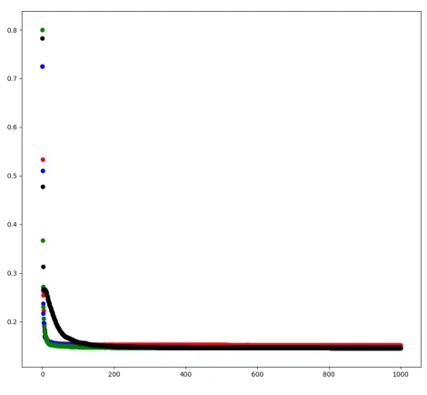
To highlight the behavior the two methods with different loss functions we selected theL1-PCA problem as an example optimization problem. The details ofL1-PCA and the dataset are highlighted in Chapter 4 but all of the various losses we used demonstrated similar behavior for the different learning rates. For these experiments we extracted the top 10 principal components from a dataset consisting of 400 25-dimensional vectors. In all of these experiments we use a learning rate schedule that reduced the learning rate by an order of magnitude at 50% and again at 75% through training. We provide example plots of the loss over the course of training with the Two-Step and PMO methods in Figures 3.4 and 3.5, respectively.
The plot in Figure 3.4 shows the significant impact the learning rate has on the Two-Step method. If the learning rate is too-high the optimizer takes excessively large steps and fails to converge, depicted by the Red and Blue plots in Figure 3.4. This verifies a key requirement in the proof of convergence for the Two-Step method: the step size must be small enough that the update is in the local region of the manifold where the tangent space is still representative. However, if the loss function is too small the optimizer will fail to converge to the global minimum, depicted by the Black plot in Figure 3.4. We found that a learning rate of 0.1 generally assured convergence to the global minimum, shown as the green plot in Figure 3.4.
Figure 3.4: Example behavior of the loss when varying the learning rate using the Two-Step retraction method. The learning rates used were: Red 10.0, Blue 1.0, Green 0.1, Black 0.01.
to accelerate the convergence of the Two-Step method using a customized learning rate schedule. We initially train with a high learning rate of 1.0 for the first 5% of training, then the learning rate is reduced by an order of magnitude at 60% and 85% through training. We found that this configuration allowed for the optimal convergence of the Two-Step method. Even with the optimized learning rate schedule, the Two-step method often takes over 2000 epochs to converge.
Figure 3.5: Example behavior of the loss when varying the learning rate using the Proxy-Matrix method. The learning rate was reduced by an order of magnitude at 50% and again at 75% through training.The learning rates used were: Red 1000.0, Blue 100.0, Green 10.0, Black 1.0.
method, we designed a learning rate schedule for PMO to accelerate convergence based on the behavior of demonstrated in the Figure 3.5. We found that PMO tends to make the majority of the reduction to the optimization loss with the largest learning rate, and only needs the learning rate to be reduced to minimize oscillation. Therefore we settled on a learning rate schedule for PMO where the learning rate was reduced by an order of magnitude at 80% and 90% through training.
3.4.2 Number of Iterations for Convergence
with various loss functions, however we will provide only a few informative results for the reprojection loss formulation of PCA with various norms. The utility of such optimization problems is discussed in Chapter 4.
In order to demonstrate the consistent improved convergences of the Proxy-Matrix method, we plot the convergence plots for optimization of three different variants of PCA in Figures 3.8, 3.7, and 3.6, where theL0.5 L1 andL2 norms are optimized, respectively. To do this we trained each optimizer for a wide range of iterations, from 1 to 10000, and report the final reprojection accuracy they achieved relative to the optimal solution. For all experiments in this section the customized learning rate schedules were used for both methods.
101 102 103 104
0 0.2 0.4 0.6 0.8 1
Epochs
Con
v
er
gence
Ratio
Two-Step Proxy-Matrix
Figure 3.6: Convergence plot of Two-Step and Proxy Matrix methods, Blue and Red plots respectively, forL2-PCA.
101 102 103 104 0.4
0.6 0.8
Epochs
Con
v
er
gence
Ratio
Two-Step Proxy-Matrix
Figure 3.7: Convergence plot of Two-Step and Proxy Matrix methods, Blue and Red plots respectively, forL1-PCA. (Note the horizontal axis is in log-scale.)
101 102 103 104
0.5 0.6 0.7 0.8 0.9 1
Epochs
Con
v
er
gence
Ratio
Two-Step Proxy-Matrix
3.5
Implementation Details
We present a neural network-based implementation of Grassmann manifold optimiza-tion for dimensionality reducoptimiza-tion based on our initial work in [102]. Many methods exist for optimization over the Grassmann manifold, but many have drawbacks in-cluding lack of flexibility or slow convergence. Many other methods for Grassmann manifold optimization require the partial derivative of the loss function either be explicitly provided or solved for using suboptimal numerical differentiation. These requirements limit the flexibility of the optimizer to be used for various loss functions. In contrast, our method leverages the auto-differentiation methods supplied in the PyTorch Deep Learning framework [108] to automatically calculate the gradients of the loss functions, allowing for much greater flexibility. The proposed approach leverages the PyTorch framework by reformulating the Grassmann manifold opti-mization problem into a neural network architecture. Our initial work in the field of manifold optimization was an implementation of the One-Step retraction method using TensorFlow Deep Learning framework [1] proposed GM-PCA method [102]. The GM-PCA method was based on the One-Step optimization method, so it did not have a theoretical proof of convergence, however we found experimental that it almost always did converge.
Linear Dimensionality Reduction (LDR) is a broad range of methods which are widely used throughout the fields of machine learning and signal processing. Broadly speaking all LDR methods share a common goal, learning a low dimensional subspace that better captures the structure of the data. Different LDR methods focus on capturing different structures or features in the low dimensional representation of the data. In this section we discuss various LDR methods and how they can be reformulated to fit in a unified LDR framework which uses our proposed Proxy Matrix Optimization method.
4.1
Background
Linear Dimensionality Reduction methods are commonly used by many machine learning and signal processing methods to both reduce the processing time and extract the nominal data from noisy signals in high-dimensional data. Of particular interest in this dissertation is the application of different LDR methods to computer vision problems. Each LDR method has a unique optimization objective,fX(R), based on
the desired structure they aim to preserve or enhance in the low dimensional space. This optimization objective is used to search for a projection matrix R ∈ Rn×p which projectsn-dimensional input data to a lowerp-dimensional space such that it minimizes the objective loss. The input data is stored in an(m×n)-dimensional matrix,X= [x1, ...x1]T, whosemrows hold then-dimensional data vectors. Thus projection of high-dimensional data,X, to the low-dimensional space performed using
to the projection matrix,R, is given as:
Y=XR (4.1)
WhereYis the low-dimensional representation of the data, with dimensions(m×p). Some dimensionality reduction methods focus on optimizing projection matrix based on the low dimensionality representation,Y. Others reproject the low-dimensional data back to the high-dimensional space using the following:
˙
X=YRT =XRRT (4.2)
This reprojection is often performed when the objective focuses on learning a repre-sentation of the data that is similar to the original input data.
For most LDR methods the projection matrix is often constrained to be an or-thonormal matrix, i.e. it satisfiesRTR=IpwhereIpis the(p×p)identity matrix. If
the matrixRconforms to this constraint, its columns are orthogonal basis vectors. The set of all orthogonal matrices belonging toRn×pis the well-studied Grassmann
Mani-foldGn×pdiscussed in Chapter 3. It therefore follows that the general dimensionality reduction optimization problem can be given as:
R∗ = arg min
R∈Gn×p
fX(R) (4.3)
The field of linear dimensionality reduction is broad, and includes a huge variety of methods, each aimed at solving a particular problem with a unique optimization formulation. In this section, we present Linear Dimensionality Reduction methods that are pertinent to this work. We aim to provide both the theoretical basis for each method, as well as the formulation for their optimization objective based on Equation (4.3).
4.1.1 Grassmann Optimization for Linear Dimensionality Reduction
Secondly the Grassmann manifold optimization approach finds all components of the projection simultaneously.
Instead of the greedy approach that is typically taken for problems such as PCA, the authors propose an iterative two-step approach to optimization on the Grassmann manifold, outlined in Section 3.3.2. The first step minimizes the loss function, and the second step retracts the updated projection matrixRback to the Grassmann manifold. This work demonstrated that though it may not be the most efficient method for L2-PCA, identical results to the traditional decomposition methods can be achieved with manifold optimization techniques. They went on to show that indeed greedy decomposition methods which are commonly used on similar dimensionality reduction methods are sub-optimal for the Linear Discriminant Analysis (LDA) problem.
This approach to Linear Dimensionality Reduction based on optimization on the Grassmann manifold serves as the inspiration for much of our work in the field of LDR using our proposed PMO manifold optimization technique.
4.1.2 L2-norm Based PCA
A great deal of work has been done onL2-norm based PCA methods [30, 110]. The L2variant of PCA is widely used because there is an efficient solution that is proven to be optimal. There are three equivalent formulations forL2-PCA optimizationfX(R),
given in Equations (4.4), (4.5), and (4.6).
The goal of the first optimization formulation ofL2-PCA, Equation (4.4), is to learn an orthogonal projection,R, of a low-dimensional surrogate of the data,S, such that the maximum amount of information inXis retained inS. WhereXis the
(m×n)matrix composedmdatan-dimensional samples,Ris a(n×p)orthogonal projection matrix, andSis a(m×p)matrix composed of thep-dimensional surrogates of themdata samples. This can be represented similarly as a by replacingSusing Equation (4.1),S=XR, resulting in an equivalent optimization problem, Equation (4.5). These two formulations are often referred to as reprojection error minimization problems.
{R∗,S∗}= arg min
R∈Gn×p,S
(kX−SRTk22) (4.4)
R∗= arg min
R∈Gn×p
(kX−XRRTk22) (4.5)
R∗ = arg max
R∈Gn×p
(kXRk22) (4.6)
4.1.3 L1-norm Based PCA Background
L2-PCA is commonly used in many applications, but it is sensitive to outliers in the dataset [77]. If the data contain outliers from a significantly different distribution, the noise has a destructive impact on the principal components. This effect is more apparent in the case of theL2-PCA because of the squared magnitude in theL2-Norm, as explained in [14].
One approach to minimizing the impact of outlying data points is to replace the L2-Norm with theL1-Norm when calculating the principal components (PCs). The drawback to using theL1-Norm is that the reprojection theorem does not hold under theL1-Norm, thus the Singular Value Decomposition (SVD) method used for the L2norm can no longer be applied. Additionally, the three corollaryL1optimization problems, Equations (4.7), (4.8), and (4.9), are no longer equivalent. Focus has primarily been on two of the formulations: reprojection error minimization, Equation (4.8), and projection energy maximization, Equation (4.9).
{R∗,S∗}= arg min
R∈Gn×p,S
(kX−SRTk1) (4.7)
R∗= arg min
R∈Gn×p
(kX−XRRTk1) (4.8)
R∗ = arg max
R∈Gn×p
(kXRk1) (4.9)
solutions have been developed in [96, 97] with computational complexityO(2N K)
andO(Nrank(X)K−K+1), respectively, whereN is the number of data points. More recently a sub-optimal but more efficient method forL1-PCA was proposed in [98]. Markopoulos et al. develop a method which greedily searches for eachL1principal component using bit flipping to find the components that m