JOURNAL OFVIROLOGY, Jan. 2005, p. 669–676 Vol. 79, No. 2 0022-538X/05/$08.00⫹0 doi:10.1128/JVI.79.2.669–676.2005
Copyright © 2005, American Society for Microbiology. All Rights Reserved.
MINIREVIEW
Basic Statistical Considerations in Virological Experiments
Barbra A. Richardson
1,2* and Julie Overbaugh
2,3Department of Biostatistics, University of Washington,1and Divisions of Public Health Sciences2
and Human Biology,3Fred Hutchinson Cancer Research Center, Seattle, Washington
INTRODUCTION AND RATIONALE
All too frequently, authors who submit manuscripts to the
Journal of Virology, and indeed to most journals, are surprised
to find that the reviewers do not share the authors’ view of their data and, as a result, do not feel that the conclusions of the manuscript are valid. Where authors see a significant dif-ference in infectivity or a significant difdif-ference in the intensity of a band on a gel, others do not. If the reviewers are uncertain about whether the proper conclusions have been drawn from the experiments, many readers will likely share that uncer-tainty. Statistical analyses can help provide a more uniform perspective of the data because they provide an objective method for determining if the differences between groups are significant, given the inherent variability of the experiment.
A recent survey of articles published in the journalInfection
and Immunityfound that about half of the 141 papers
exam-ined contaexam-ined errors in statistical analyses and/or reporting of results (10). In a quick perusal of last year’sJournal of Virology
papers, we saw similar problems in articles describing studies ranging from basic laboratory experiments, such as viral infec-tion studies, to vaccine studies that purport to show efficacy. For example, only half of the AIDS-related vaccine papers in the last issues of 2003 used and reported on statistical testing appropriately (2, 7, 12). These observations suggest that the term “significant difference” is often being misused and that statistical support for such a conclusion is often lacking across many types of virological studies.
Here, we review some of the basic considerations that may be relevant to the statistical analyses of data from virological experiments. Following the diagram presented in Fig. 1, we first discuss study design and why statistical considerations are important even before one goes to the bench to start an ex-periment. Second, we provide an outline of the basic summary statistics that typically are used when reporting the results of experiments common to virologists. Third, we outline basic considerations for testing hypotheses and selecting a method of statistical testing for one’s data. Finally, we provide guide-lines for interpreting the results of statistical testing. After this central discussion of statistical considerations, we then use some hypothetical studies to further illustrate these concepts: the first, a vaccine study in animals; the second, the
character-ization of a viral mutant in vitro. Important statistical terms used throughout the paper are defined in Table 1, and several textbooks that cover basic statistical concepts are included in the reference section (1, 4, 5, 8, 9, 11). With this review we hope to help virologists present data more objectively and rigorously and provide sufficient information to help readers evaluate whether the conclusions of a paper are supported by the data presented. The use and reporting of appropriate sta-tistical testing also help readers to better compare outcomes from different studies and to determine if the conclusions of a study are valid.
BASIC CONSIDERATIONS FOR VIROLOGICAL EXPERIMENTS: STUDY DESIGN, DESCRIBING DATA,
ANALYZING DATA, AND REPORTING OF ANALYSIS RESULTS
Study design.Traditionally, the first step in many research projects is developing a hypothesis based on scientific reason-ing to guide how the experiments are conducted—that is, the study design. The hypothesis guides decisions not only about what type of data to collect but also about what amount of data is needed to detect a significant difference.
Significance level and power are crucial concepts for both study design and statistical testing of scientific hypotheses. The significance level is defined as the probability of falsely finding a statistically significant difference and, in practice, is typically fixed at 0.05 (so that when performing statistical testing, P
values of less than or equal to 0.05 are defined as indicating a statistically significant difference; see “Results of statistical testing of hypotheses:Pvalues”). Power is defined as the prob-ability of detecting a statistically significant difference that truly exists. Four factors important in study design can increase the power of a test. They are (i) an increase in the sample size, (ii) an increase in the expected magnitude of the difference be-tween the groups, (iii) a decrease in the expected spread of the samples, and (iv) an increase in the significance level of the test.
In the context of any given experiment, some of these factors may be difficult to adjust, but a well-considered study design can help. Consider an experiment comparing the infectivity of mutant versus wild-type viruses, where if we expect a relatively subtle effect of the mutation on infectivity we could increase power by using an assay that requires multiple rounds versus a single round of virus replication. More commonly, though, the power to detect a difference could most readily be increased by improving the reproducibility of the assay to decrease variation in the data (and thereby decrease the spread of the sample)
* Corresponding author. Mailing address: Harborview Medical Cen-ter, University of Washington, Box 359909, 325 Ninth Avenue, Seattle, WA 98104-2499. Phone: (206) 731-2425. Fax: (206) 731-3693. E-mail: [email protected].
669
on November 8, 2019 by guest
http://jvi.asm.org/
and/or by increasing the number of replicates of the assay to increase the sample size. These considerations in the study design lead to an increase in the power of the study to detect an effect and to conclusions that are more robust.
The importance of statistical considerations in study design can be further illustrated by using the example of vaccine studies in animals. In such studies, the ideal test of the efficacy of a vaccine is presence versus absence of infection. Therefore, a study in which one wants to prove efficacy requires enough power to detect a statistically significant difference in the pro-portion of animals infected in a treated group versus those
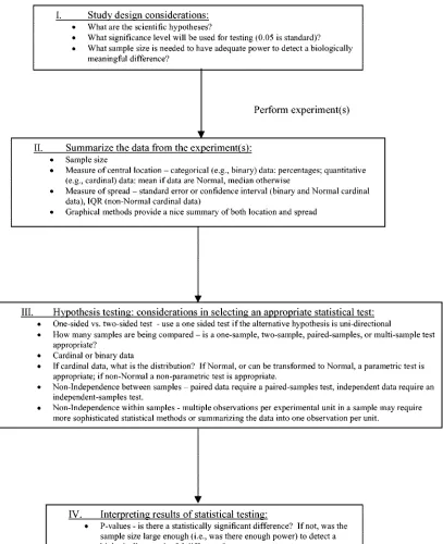
[image:2.585.89.496.66.566.2]infected in a control group. As seen in Table 2, if such an experiment is designed with only three animals in each group, the results will never reach statistical significance (P⬍0.05), even if all control animals become infected and all treated animals escape infection. With such a small group, there is simply not enough data to be confident that there is a differ-ence; that is, there is insufficient statistical power. However, with as few as five animals per group, we could detect a sig-nificant difference even if one control animal remains unin-fected or one treated animal becomes inunin-fected. Thus, the con-sideration of statistical issues such as significance level and
FIG. 1. Flow diagram of basic statistical considerations in virological experiments. IQR, interquartile range.
on November 8, 2019 by guest
http://jvi.asm.org/
power during study design results in less waste of time and resources and allows scientists to objectively draw conclusions from the data collected.
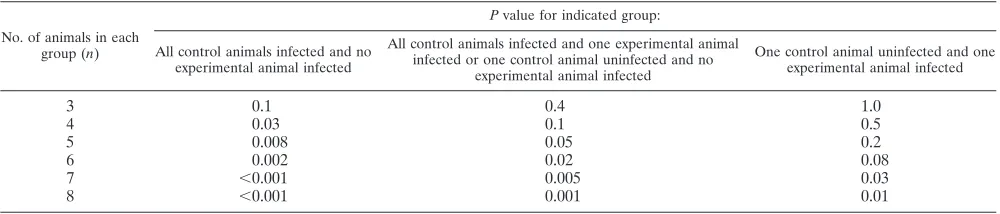
Description of data: summary statistics. Once the experi-ments are completed, the next step is to provide a concise description of the data through the use of summary statistics that include the sample size and measures of location and spread. This description should be presented separately for each experimental (and control) group in the study; for exam-ple, it should be presented separately for wild-type and mutant viruses. If the results are categorical (e.g., from a qualitative assay), they can easily be described by presenting the number of results that fall into each outcome category. For example, we could report (i) the number of PCRs of a sample that yielded a product that could be detected on a gel and (ii) the number of PCRs that did not. For quantitative data (e.g., cardinal data), however, there are several factors to consider when deciding which summary statistics should be presented. While graphs are usually a good way of presenting summary statistics, any presentation of summary statistics is incomplete without a clear description of (i) the size of each sample, (ii) a summary measure of the central location of each sample, and (iii) a summary measure of the spread of each sample. Figure 2A shows an example of this type of summary in a format that is common in theJournal of Virologyand that contains these three elements. Below are some considerations regarding the
presentation and selection of summary statistics for describing the data.
(i) Sample size. Sample size is defined as the number of experimental units in each group. In the case where we are assessing differences in infectivity between a wild-type virus and mutant virus(es), the sample sizes that should be relayed to the reader are the number of experiments we performed for each virus. For example, Fig. 2A indicates that there are seven experiments measuring infectivity (infectious units/ml [IU/ml]) for the wild-type virus, five experiments measuring infectivity for the mutant A virus, and eight experiments measuring in-fectivity for the mutant B virus. Stating the sample size within an experiment is crucial, since, as mentioned above, sample size is one of the factors that affect the power of any experi-ment.
[image:3.585.43.543.601.708.2](ii) Measures of central location.The mean (average value) and median (middle value) are used to define the center of a sample of data. Which of these two measures best summarizes the data can be hard to determine and often depends on the subject matter. It is important to keep in mind that the sample mean is very sensitive to extreme values, whereas the median is not. When the distribution of data points is not symmetrical, the mean and median of a sample will differ. Using different definitions of the center of the sample can lead to very different interpretations of the data. However, in many cases of non-symmetrical distributions, the data can be transformed (e.g.,
TABLE 1. Statistical terms
Term Definition
Alternative hypothesis...Hypothesis that contradicts the null hypothesis
Binary data ...Data that consist of only two values (e.g., positive, negative) Cardinal data...Data that are on a scale in which common arithmetic is meaningful Confidence interval ...Likely range of the true value of a parameter of interest
Hypothesis testing...Use of statistical testing to objectively assess whether results seen in experiments are real or due to random chance
Nonparametric test...Statistical test that requires no assumptions regarding the underlying distribution of the data
Normally distributed data...Data which, when plotted in a histogram, look approximately like a bell-shaped curve Null hypothesis...Scientific hypothesis that one wants to test (if hypothesis testing results in a statistically
significant difference, the null hypothesis is rejected)
Pvalue...Probability of getting a result as extreme as or more extreme than the value obtained in one’s sample, given that the null hypothesis is true
Parametric test ...Statistical test that assumes the data follow a particular distribution (e.g., normal) Power ...Probability of detecting a statistically significant difference that truly exists Sample size ...Number of experimental units in a study
Significance level...Probability of falsely finding a statistically significant difference
TABLE 2. Pvalues for the differences in infection rates between experimental and control groupsa
No. of animals in each group (n)
Pvalue for indicated group:
All control animals infected and no experimental animal infected
All control animals infected and one experimental animal infected or one control animal uninfected and no
experimental animal infected
One control animal uninfected and one experimental animal infected
3 0.1 0.4 1.0
4 0.03 0.1 0.5
5 0.008 0.05 0.2
6 0.002 0.02 0.08
7 ⬍0.001 0.005 0.03
8 ⬍0.001 0.001 0.01
aDetermined by Fisher’s exact test, using a two-sided hypothesis test with the significance level fixed at 0.05. Fisher’s exact test is used because it is appropriate for
experiments with small numbers of observations.
VOL. 79, 2005 MINIREVIEW 671
on November 8, 2019 by guest
http://jvi.asm.org/
symmetrical distribution of the sample data, thereby making the two measures of central location similar. For example, the wild-type virus infectivity measures presented in Fig. 2A con-tain one data value of 10,000 IU/ml, which is very different from the rest of the measurements. Hence, the mean IU/ml for the seven measurements of the wild-type virus is 2,195 (Fig. 2A), whereas the median is 956 (not shown)—two very differ-ent numbers, with the larger mean exemplifying the sensitivity of this summary statistic to extreme values. However, in Fig. 2B, in which the same data has been transformed to log10
IU/ml, we see that the mean log10IU/ml for the wild-type virus
is 3.1 and the median is 3.0 (not shown). The similarity of these numbers indicates that the log transformation has made the distribution of these data more symmetrical and the definition of the center of the sample more consistent. In such cases, it is usually preferable to work with these transformed values when analyzing data, especially if we are working with analysis meth-ods that assume a symmetrical distribution of the data; i.e., that the data, when plotted in a histogram, look approximately like a bell-shaped curve (also referred to as a normal distribution). Finally, as a general rule, it is important that the summary measure of central location that is presented to the reader be compatible with the test used for statistical analysis of the data. For example, if we use an independent-samplesttest (Table 3), the mean of each group should be reported; if we use a paired
ttest (Table 3), the mean difference between pairs should be reported; and if we use a test that is resistant to outliers (e.g., the Wilcoxon rank sum test; Table 3), the median of each group should be reported. Each statistical test is designed specifically for use with a particular summary statistic. Using a test such as the paired ttest to test for differences between medians would be like using RNA PCR to estimate the level of protein expression—scientifically inappropriate.
(iii) Measures of spread. When using the sample mean as the summary measure of location, the standard deviation, the sample standard error of the mean, or a confidence interval (see “Analyzing data: hypothesis testing”) should be used as a summary measure of spread (Fig. 2). The sample standard error of the mean is defined as the standard deviation of the observations divided by the square root of the sample size. When the sample median is used as the summary estimate of location, the sample interquartile range (the 25th and 75th percentiles) should be reported. For example, using the un-transformed IU/ml data for the wild-type virus in Fig. 2A, the interquartile range of the data is 756 to 1,200 (not shown).
[image:4.585.56.272.60.720.2]Analyzing data: hypothesis testing.Statistical considerations are key not only to an experiment’s design and implementation but also to an objective interpretation of its results. Simply
FIG. 2. Comparison of the infectivity of the wild-type virus and that of two mutant viruses. The bars show the means, and the error bars show⫾1.0 standard error of the mean. (A) The mean IU/ml and the standard error of the mean for each of the three viruses on a linear scale. (B) The mean log10IU/ml and the standard error of the mean for each of the three viruses on a log10scale. (C) The mean log10IU/ml and the standard error of the mean for each of the three viruses and the results from formal statistical hypothesis testing, assuming inde-pendence between measurements of the infectivity of the wild type, mutant A, and mutant B. *,Pvalues were computed by using two-sided independent samplettests and comparing the results to those for the wild type.
672
on November 8, 2019 by guest
http://jvi.asm.org/
providing a summary measure of location and a summary mea-sure of spread (Fig. 2A), as many articles do, is not enough to prove statistically significant differences between groups. A common mistake is to place error bars (⫾1 standard error) around the means of different groups and to state that two groups are different if the lower error bar from one group falls above the upper error bar of the other group (Fig. 2A and B). Error bars and 95% confidence intervals convey an interval measure of the precision of the estimated group mean, but overlapping 95% confidence intervals are not sufficient to prove a lack of statistical significance, and mutually exclusive error bar intervals are not sufficient to prove a statistically significant difference.
Error bars and 95% confidence intervals provide a nice description of precision but should not be overinterpreted; they simply convey the amount of uncertainty in the true mag-nitude of the mean. By definition, if the distribution of the data is normal, we can state that, if we take repeated random sam-ples of the same size from the population of interest, 95% of the 95% confidence intervals of these samples will contain the true mean of the population. Using error bars (⫾1 standard error) to create an interval is equivalent to constructing a 68.3% confidence interval and can be interpreted as such (as-suming normal data). Therefore, error bars and 95% confi-dence intervals, while useful for describing data (Fig. 2A and B), are insufficient unless accompanied by the results of formal hypothesis testing. This rule is illustrated by Fig. 2C and dis-cussed below, where we present some considerations relevant to testing hypotheses using statistical analysis methods, some definitions of terms encountered when performing statistical tests, and some guidelines regarding which tests may be ap-propriate in different data situations.
(i) Formulating hypotheses: one-sided versus two-sided tests.A hypothesis based upon scientific reasoning will deter-mine whether a one-sided or a two-sided statistical test is better suited to an experiment. For example, suppose we are interested in determining if infected macaques who were given a vaccine have lower viral-replication levels at 6 weeks after
infection than infected macaques given a placebo, and we assume that higher viral-replication levels in the vaccinated animals would be interpreted as an indication that the vaccine had no benefit of interest. In this case, two potential hypoth-eses are (i) that the vaccine has no beneficial effect on the viral-replication levels at 6 weeks after infection and (ii) that the vaccine lowers the viral-replication levels by 6 weeks after infection. In statistical terms, this first hypothesis is the null hypothesis and the second one is the alternative hypothesis. In this example, according to the hypotheses, we do not care if the vaccine increases these levels; the interest is in only one direc-tion: whether it lowers the viral-replication levels or not. Such hypotheses, in which the alternative hypothesis is unidirec-tional, are called one-sided hypotheses and call for one-sided statistical tests.
Alternatively, suppose we are interested in determining if a vaccine has any effect on viral-replication levels, regardless of the direction of that effect. In this case, the two hypotheses are (i) that the vaccine has no effect on the viral-replication levels at 6 weeks after infection and (ii) that the vaccine either in-creases or dein-creases the viral-replication levels at 6 weeks after infection. Such hypotheses, in which the alternative hypothesis is bi-directional, are called two-sided hypotheses and call for two-sided statistical tests.
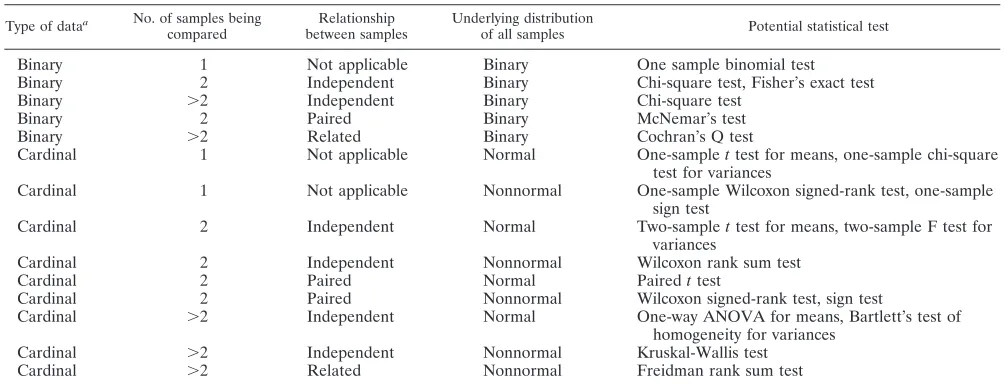
(ii) Statistical testing of hypotheses: one-sample tests, paired-sample tests, two-sample tests, and multisample tests.
[image:5.585.41.543.88.281.2]Statistical testing is called for in many types of virological experiments, including those that compare a variety of differ-ent biological properties of two viruses (infectivity, enzymatic activity, expression levels, binding, antigenicity, etc.). Such studies may be broadly categorized into those where a single virus is analyzed in relation to a standard level, such as wild-type activity, and those where two or more viruses are com-pared directly. One-sample tests (e.g., one-samplettest, one-sample binomial test; Table 3) are appropriate for the first category of study, whereas two-sample or multisample tests (e.g., paired t test, two-sample t test, analysis of variance [ANOVA]; Table 3) are appropriate for the second category.
TABLE 3. Potential statistical testing methods for various types of data (assuming that observations within samples are independent of one another)
Type of dataa No. of samples being
compared
Relationship between samples
Underlying distribution
of all samples Potential statistical test
Binary 1 Not applicable Binary One sample binomial test
Binary 2 Independent Binary Chi-square test, Fisher’s exact test
Binary ⬎2 Independent Binary Chi-square test
Binary 2 Paired Binary McNemar’s test
Binary ⬎2 Related Binary Cochran’s Q test
Cardinal 1 Not applicable Normal One-samplettest for means, one-sample chi-square test for variances
Cardinal 1 Not applicable Nonnormal One-sample Wilcoxon signed-rank test, one-sample sign test
Cardinal 2 Independent Normal Two-samplettest for means, two-sample F test for
variances
Cardinal 2 Independent Nonnormal Wilcoxon rank sum test
Cardinal 2 Paired Normal Pairedttest
Cardinal 2 Paired Nonnormal Wilcoxon signed-rank test, sign test
Cardinal ⬎2 Independent Normal One-way ANOVA for means, Bartlett’s test of
homogeneity for variances
Cardinal ⬎2 Independent Nonnormal Kruskal-Wallis test
Cardinal ⬎2 Related Nonnormal Freidman rank sum test
a
Binary, data with only two categories (0,1); cardinal, data that are on a scale in which common arithmetic is meaningful.
VOL. 79, 2005 MINIREVIEW 673
on November 8, 2019 by guest
http://jvi.asm.org/
We would use a one-sample test, for example, to compare the levels of expression or enzymatic activity of a mutant pro-tein to that of the wild-type propro-tein on a single gel. In this case, the levels for the wild type are typically set at 100% within each experiment, and data from experiments (e.g., gels) performed on different days are not pooled because the conditions of each experiment will systematically affect the absolute levels for both the wild type and the mutant. Authors then often pick a single experiment to present, one that they feel best represents their data. However, it would be more appropriate to report the results of formal hypothesis testing because it offers an objective and consistent basis for the interpretation of all the experiments together rather than reliance on an individual’s determination of representative data. To do so, we would use a one-sample test on a summary measure (e.g., a one-samplet
test on the mean or log10 mean) of the ratios of mutant to
wild-type levels derived from multiple replications of the ex-periment to determine if the ratio of mutant to wild-type levels is significantly different than 1.
We would use a paired-sample, two-sample, or multisample test, for example, when we wanted to determine whether the introduction of a mutation in a viral gene alters its infectivity. In this case, the number of infectious particles, as determined by replicate infection assays (often performed in parallel), of wild-type versus mutant virus(es) would be compared. If the experiment is designed to collect paired data (for example, if each measurement of IU/ml of wild-type virus is paired with a measurement of IU/ml of mutant virus from the same exper-iment), hypothesis testing should be performed by using a paired-sample test on a summary measure of the infectious particles (e.g., for the mean, a pairedttest), but if the exper-iment is designed to collect independent data on the different viruses (for example, if data for each virus is collected on different days by using independent virus preparations tested in independent experiments), two-sample or multisample tests for independent groups should be performed on a summary measure (e.g., for the mean, a two-samplettest or an ANOVA) of the infectious particles. These rules are discussed in more detail in the section on independence of data measurements below.
(iii) Statistical testing of hypotheses: type of data.The type of data collected in an experiment is another key consideration in the choice of which statistical test to use. While there are exceptions, most data collected in virological experiments can be defined as either (i) binary, that is, consisting of two distinct categories (e.g., positive and negative), or (ii) cardinal, that is, quantitative and on a scale in which common arithmetic is meaningful (e.g., IU/ml). In the example of the vaccine studies mentioned above, the ideal test of efficacy is presence versus absence of infection. The outcome data from this type of ex-periment is binary (infected/uninfected), and a statistical test appropriate for binary data should be used (e.g., Fisher’s exact test or chi-square test; Table 3). On the other hand, if the interest in the vaccine study is to compare viral RNA levels, the outcome data from the experiment are cardinal. In this case, a statistical test appropriate for cardinal data (e.g., two-samplet
test; Table 3) should be used.
(iv) Statistical testing of hypotheses: parametric testing ver-sus nonparametric testing.While an experiment’s hypothesis and design narrows down the number of appropriate statistical
tests available, often the decision of exactly which statistical test to use is still not obvious when we have cardinal data. Parametric tests, such as thettest, linear regression analysis, ANOVA, and the F test, assume that the data being analyzed follow an underlying known distribution. For example, thet
test assumes that the underlying distribution of the data is normal. However, if we cannot make an assumption regarding the underlying distribution of the data, nonparametric tests, such as the Wilcoxon rank sum test (Table 3), can be per-formed. Nonparametric tests, however, are less powerful than parametric tests if the distributional assumptions of the para-metric test hold.
(v) Statistical testing of hypotheses: independence of data measurements between and within groups.Finally, when se-lecting a method of statistical analysis, we should also consider whether or not the data measurements from the experiment are independent from each other. Independence can be differ-entiated into two types: between groups and within groups. The former occurs when the observations in each group being compared are independent of observations in the other groups. Take the experiment comparing viral-replication levels in vac-cine-treated and placebo-treated macaques. Because different animals were treated with the vaccine and the placebo, the data are independent between groups and call for a statistical test that assumes this kind of independence, such as the indepen-dent-samplesttest or the Wilcoxon rank sum test (Table 3). However, if the animals were paired based on age and sex and one member of each pair was randomly selected to receive the vaccine and the other member to receive the placebo, the data for the vaccine-treated and placebo-treated groups would not be independent. Rather, the data would be paired and would call for a statistical test for paired data, such as the pairedttest or the sign test (Table 3).
The second type of independence, independence within groups, occurs when the observations in each group are inde-pendent of other observations in that same group. An absence of this type of independence is common in virological experi-ments, since viral or immune kinetics are often of interest. For example, suppose we are looking at viral replication levels at 4, 6, and 8 weeks after infection in the vaccine versus placebo macaque experiment described above, or suppose we are look-ing at viral replication in culture over time. In such cases, because we have multiple observations per experimental unit (i.e., animal or virus), the data within each group are not independent and the standard statistical methods outlined in Table 3 do not apply. If the data follow certain assumptions, we can use more-complex statistical modeling techniques, such as random effects models, generalized estimating equations, or repeated measures ANOVA, most of which are best per-formed in consultation with a statistician. However, an easier but potentially less powerful method of quantifying viral or immune kinetics is to simplify the data over time into a sum-mary measure, such as the area under the curve minus the baseline value, and perform less-complex statistical testing on these values (6).
Results of statistical testing of hypotheses: P values. The results of formal statistical testing are most often summarized in the form of aPvalue. ThePvalue is defined as the proba-bility of getting a result as extreme as or more extreme than the value obtained in one’s sample, given that the null hypothesis
on November 8, 2019 by guest
http://jvi.asm.org/
is true. Let us again consider the data presented in Fig. 2 and now determine whether the infectivity of the wild-type virus was significantly different from the infectivity of mutant A or from the infectivity of mutant B. Let’s assume that there is no indication of whether we should hypothesize that the wild type will be more infectious or less infectious than mutant A. Then a two-sided hypothesis test is appropriate, and we can use an independent-samplesttest with the significance level fixed at 0.05 on the log10transformed data to test for differences in the
mean infectivity of the wild type and mutant A. Doing so gives aPvalue of 0.1, indicating that if the wild type and mutant A do not have distinguishable infectivity (i.e., the null hypothesis is true) then the probability that we will see a difference as large as or larger than the difference between the wild type and mutant A obtained in this particular experiment is 0.1. Similar testing comparing the wild-type virus to mutant B gives a
Pvalue of 0.04, which can be defined in the same manner (Fig. 2C). So, although the mean levels of infectivity of mutant A and mutant B look similar and appear to be significantly lower than that for the wild-type virus (Fig. 2A and B), with formal statistical testing we find only a trend for significantly lower infectivity for mutant A compared to that for the wild type (Pvalues between 0.05 and 0.10 can be interpreted as indicat-ing a trend toward statistical significance). With mutant B, however, we are able to detect a significant difference com-pared to the wild type (P⬍0.05). In this case, the difference in significance here is mainly due to a larger sample size for mutant B (n⫽8), giving this experiment more power to detect a difference (Fig. 2C).
EXAMPLE STUDIES
Example 1: a vaccine study in animals. Suppose we are testing a vaccine in a simian immunodeficiency virus model by randomizing independent animals to vaccine or placebo, and we hypothesize that the vaccine will not block infection but will attenuate the disease course. In fact, the types of outcomes measured are often similar across studies comparing vacci-nated to unvaccivacci-nated animals, treated to untreated animals, or animals infected with different variant or mutant viruses. These outcome measures include some measure of virus rep-lication, which is often viral RNA or DNA levels in blood, immune responses (both cellular and humoral), and clinical markers, such as CD4 counts. Considerations in selecting a method for statistical analysis include (i) the type of outcome data, (ii) whether or not the data within a group follow an approximately normal distribution, (iii) whether the measure-ments between and within groups are independent, and (iv) whether the results from statistical testing should be adjusted for multiple comparisons.
In applying these considerations to vaccine studies, we see first that the outcome data are generally cardinal, calling for the corresponding statistical methods (Table 3). Second, log10
-transformed values may be more useful than un-transformed values, particularly for measures of viral replication, if the transformation changes the data to an approximately normal distribution, as this will allow us to utilize parametric testing methods for normally distributed data. Third, in animal studies where viral or immune levels are measured over time, the data within a group are not independent because we have multiple measurements per animal. In such cases, either the data must
be simplified into a single summary measure per animal (e.g., initial set point viral RNA level) or more complicated statisti-cal methods must be employed (as discussed above). Finally, when several groups are compared at once, an adjustment for multiple comparisons may be needed to account for the chance that if one makes enough comparisons one of them will show a statistically significant difference. However, there is not com-plete consensus in the statistics community concerning which situations call for such an adjustment and, if so, which to use (see reference 3 for a review and reference 7 for an example).
Example 2: comparison of wild-type and mutant viruses.
Take another experiment common in virology, where the struc-ture and function of a viral protein is assessed by engineering specific mutations at residues that are hypothesized to be part of the functional domain of the protein. If, for example, we construct a mutation in a protease gene that we hypothesize will abate function, four experiments are performed to deter-mine (i) whether the expression levels of the wild-type and mutant viruses differ, (ii) whether the protease activity of the wild-type and mutant viruses differ, (iii) whether the infectivity of the wild-type and mutant viruses differ in a single-cycle assay, and (iv) whether the replication kinetics of the two viruses over time are different.
First, to determine whether the steady state expression levels of the wild-type and mutant viruses differ, we run several in-dependent experiments using Western blotting. Within each experiment (each of which has a mock control which yielded no signal) we obtain expression levels for the wild-type virus and the mutant virus. Setting the wild-type level within each experiment as the standard (i.e., at 100%), we obtain a value for mutant virus expression: the ratio of the mutant level to the wild-type level in each experiment. So, for this part of our study, we have several independent cardinal measurements (the ratios) of the expression level of the mutant virus com-pared to that of the wild-type virus, and we want to determine if these ratios are significantly different than 1. If not enough experiments are performed to know if the data follow a normal distribution, as is typically the case, we would use a one-sample Wilcoxon signed-rank test to determine if the ratios are signif-icantly different than 1. However, if we do have sufficient data to demonstrate that the ratios are normally distributed, we can use the more powerful one-samplettest (Table 3). Alterna-tively, instead of taking the ratio of mutant expression level to wild-type expression level within each experiment, we can treat these two values within each experiment as paired data and use a pairedttest, sign test, or Wilcoxon signed-rank test, depend-ing on the approximate distribution of the data.
Second, to determine whether the protease activity of the wild-type and mutant viruses differ, we perform several inde-pendent experiments where we take a substrate and determine how much of it is cleaved by the wild-type protease, mutant protease, and a negative control (mock). Sometimes the results of such an experiment are obvious, such as when in each experiment the substrate is nearly completely cleaved by the wild-type enzyme and there is no detectable cleavage by the mutant. In such cases, statistical testing only confirms the ob-vious. However, in many cases the activity of the mutant is reduced more modestly and statistical tests are more critical for drawing conclusions. If the mock has no cleaved product, the data from these experiments can be treated as we treated
VOL. 79, 2005 MINIREVIEW 675
on November 8, 2019 by guest
http://jvi.asm.org/
the cardinal data from our experiments to determine expres-sion levels: e.g., we can treat the wild-type activity as the stan-dard and perform statistical testing on the ratios of the values for mutant activity to wild-type activity or treat the two values for protease activity as paired observations within each exper-iment and use statistical methods for paired data. The situation is a bit more complicated if there is cleaved product in the mock experiment, and this result must be considered in the analyses to account for cleavage that occurs in the absence of enzyme. In this case, the simplest option, if appropriate under the experimental conditions, is to subtract the value for mock activity from those for both mutant and wild-type activity and proceed with statistical analyses of the ratios of mutant to wild-type activity as described above. Otherwise, the data on the ratio of cleaved product to total product for the mock, wild type, and mutant within each experiment should be considered nonindependent data, and depending on the approximate dis-tribution of the ratio data, pairedttests (with adjustments for multiple comparisons) or a Friedman rank sum test could be used to test for differences between the mock, wild type, and mutant ratios.
Third, to determine if the infectivity of the wild-type and mutant viruses differs in a single-cycle assay, we perform sev-eral independent experiments, measuring the IU/ml for wild type and mutant (in parallel) multiple times (e.g., in triplicate). From each of these experiments, we calculate the mean IU/ml for the wild type and the mean IU/ml for the mutant. Then, a pairedttest, sign test, or Wilcoxon signed-rank test (depending on the approximate distribution of the data) could be used to test for differences between the infectivity of the wild type and the mutant, based on calculated means. Alternatively, if each individual measurement of infectivity (rather than the means) were used for analyses, more complex methods, such as gen-eralized estimating equations, would be necessary to account for the correlation (nonindependence) between observations within each experiment.
Finally, to determine if the replication kinetics of the two viruses over time are different, we can measure the virus pro-tein levels for both the wild type and the mutant every 2 days for 2 weeks, with triplicate measures of protein levels at each time point. However, we must keep in mind that, even if we summarize data from each time point into a single measure (e.g., the mean), the data within each group (wild type and mutant) are not independent, as we have multiple measures per virus. This situation is similar to that in Example 1, for which we had multiple measurements per animal. Therefore, statistical analyses of differences in replication kinetics can be handled the same way. That is, either the data must be sim-plified into a single summary measure per virus (e.g., peak levels of virus production), allowing statistical methods appro-priate for two groups to be used to compare wild-type and mutant levels (Table 3), or more complicated statistical meth-ods must be employed (as discussed above).
SUMMARY
Some experimental results, such as cases where mutations nearly abolish infectivity or enzymatic activity, may be suffi-ciently clear so that statistical methods are not needed to form a consensus among scientists regarding the conclusions. How-ever, when the effects are more subtle, statistical methods,
starting with a study design with sufficient power to detect significant differences, can be critical for drawing conclusions that are generally accepted by the research community as a whole. At as early as the experimental design stage, it is im-portant to have statistical considerations such as sample size, power, significance level, and the appropriate statistical tests in mind so that one has a better chance of truly answering the scientific hypotheses of interest. Once data are collected, a description of the data (e.g., summary statistics) and an accu-rate presentation of the results of statistical testing are neces-sary so that readers may objectively assess the study. Finally, a detailed description of how statistical analyses were performed (preferably in the methods section of the paper) is just as important as a description of laboratory methods, because the absence of details on statistical or laboratory methods make it difficult for the reader to evaluate the quality of the study. While the basic considerations are covered here, more-com-plex data, study design issues, and analyses may require con-sultation with a statistician. As virologists continue to incorpo-rate more quantitative and/or high-throughput methods into their research, statistical methods will become even more es-sential for interpreting data and drawing conclusions that oth-ers can undoth-erstand. Clarity in the interpretation of experi-ments through proper statistical methods is the key to objectively and consistently assessing whether observed biolog-ical differences are real or due to random chance.
ACKNOWLEDGMENTS
We thank Gretchen Strauch, Michael Emerman, Nancy Haigwood, James Hughes, Sarah Benki, Heather Cheng, Mario Pineda, Bhavna Chohan, Dara Lehman, and her dad for their reviews and comments on various drafts of this manuscript and Karen Peterson for suggesting several useful texts for reference.
The authors are supported by NIH grants AI32518 and AI29168; J.O. is an Elizabeth Glaser Scientist.
REFERENCES
1.Armitage, P., G. Berry, and J. N. S. Matthews.2002. Statistical methods in medical research, 4th ed. Blackwell Science Ltd., Oxford, United Kingdom. 2.Doria-Rose, N. A., C. Ohlen, P. Polacino, C. C. Pierce, M. T. Hensel, L. Kuller, et al.2003. Multigene DNA priming-boosting vaccines protect ma-caques from acute CD4⫹-T-cell depletion after simian-human immunodefi-ciency virus SHIV89.6P mucosal challenge. J. Virol.77:11563–11577. 3.Feise, R. J.2002. Do multiple outcome measures require p-value
adjust-ment? BMC Med. Res. Methodol. 2:8.
4.Fisher, L., and G. Van Belle.1993. Biostatistics: a methodology for the health sciences. J. Wiley, New York, N.Y.
5.Freedman, D., R. Pisani, R. Purvis, and A. Adhikari.1997. Statistics, 3rd ed. W. W. Norton and Co., Inc., New York, N.Y.
6.Journot, V., G. Chene, P. Joly, M. Saves, H. Jacqmin-Gadda, J. M. Molina, et al.2001. Viral load as a primary outcome in human immunodeficiency virus trials: a review of statistical analysis methods. Control. Clin. Trials
22:639–658.
7.Kong, W.-P., Y. Huang, Z.-Y. Yang, B. K. Chakrabarti, Z. Moodie, and G. J. Nabel.2003. Immunogenicity of multiple gene and clade human immuno-deficiency virus type 1 DNA vaccines. J. Virol.77:12764–12772.
8.Moore, D. S., and G. P. McCabe.2003. Introduction to the practice of statistics, 4th ed. W. H. Freeman & Co., New York, N.Y.
9.Motulsky, H.1995. Intuitive biostatistics. Oxford University Press, New York, N.Y.
10.Olsen, C. H.2003. Review of the use of statistics inInfection and Immunity. Infect. Immun.71:6689–6692.
11.Rosner, B.2000. Fundamentals of biostatistics, 5th ed. Duxbury, Pacific Grove, Calif.
12.Vogel, T. U., M. R. Reynolds, D. H. Fuller, K. Vielhuber, T. Shipley, J. T. Fuller, et al.2003. Multispecific vaccine-induced mucosal cytotoxic T lym-phocytes reduce acute-phase viral replication but fail in long-term control of simian immunodeficiency virus SIVmac239. J. Virol.77:13348–13360.