LiDAR data for DEM generation and flood plain mapping

(1)

University of Southern Queensland

Faculty of Health, Engineering and Sciences

LiDAR Data for DEM

Generation and

Flood Plain Mapping

A dissertation submitted by

Michael James Topp

In fulfilment of the requirements of

Courses ENG4111 and ENG4112 Research Project

Towards the degree of

Bachelor of Spatial Science (Surveying)

Submitted:

(2)

0061019385 i

Abstract

On Monday 10 January 2011, a 1 in 100 year storm cell quickly developed

over the Toowoomba city dumping intensive rain in a short period of time in

the Gowrie Creek catchment (ICA, 2011). This caused extensive flash

flooding over the entire catchment including West Creek before destroying

the central business district and causing loss of life. To ensure that damage is

reduced and lives are saved in the future, areas requiring mitigation need to

be identified. To identify these areas characteristic analysis, slope analysis,

flood plain mapping and hydrological modelling can be utilised. To complete

this highly accurate Digital Elevation Models (DEM) generated from

Airborne Light Detection and Ranging (LiDAR) data can be utilised. LiDAR

is a surveying technology that can collect large amounts of accurate data

compared to traditional survey methods. Stream networks and catchment

boundaries were generated utilising Arc Hydro at multiple different

thresholds. Slope analysis was also completed highlighting the flood plain

and the possible effects of urbanisation. Hydrological modelling using the

Storm Water Management Model (SWMM) also showed extensive velocities

and volumes with assumptions. These results showed that West Creek had

extensive problems with urbanisation throughout the catchment. It also

highlighted the issues with West Creek and East Creek meeting and the

inability of the system to handle both creeks flood waters once they merge.

To proactively mitigate floods analysis should be completed before floods

(3)

0061019385 ii

Disclaimer

University of Southern Queensland

Faculty of Health, Engineering and Sciences

ENG4111 and ENG4112 Research Project

Limitations of Use

The Council of the University of Southern Queensland, its Faculty of Health, Engineering & Sciences, and the staff of the University of Southern Queensland, do not accept any responsibility for the truth, accuracy or completeness of material contained within or associated with this dissertation.

Persons using all or any part of this material do so at their own risk, and not at the risk of the Council of the University of Southern Queensland, its Faculty of Health, Engineering & Sciences or the staﬀ of the University of Southern Queensland.

This dissertation reports an educational exercise and has no purpose or validity beyond this exercise. The sole purpose of the course pair entitled “Research Project” is to contribute to the overall education within the student’s chosen degree program. This document, the associated hardware, software, drawings, and other material set out in the associated appendices should not be used for any other purpose: if they are so used, it is entirely at the risk of the user.

Dean,

(4)

0061019385 iii

Certification

I certify that the ideas, designs and experimental work, results, analyses and

conclusions set out in this dissertation are entirely my own eﬀort, except where otherwise indicated and acknowledged.

I further certify that the work is original and has not been previously

submitted for assessment in any other course or institution, except where

speciﬁcally stated.

Michael James Topp

Student Number: 0061019385

(5)

0061019385 iv

Acknowledgements

I would first like to acknowledge my supervisor for this project, Dr Xiaoye

Liu. Her expertise in this field is unquestionable and without which, I would

not have been able to complete this research project.

I would also like to acknowledge and thank the Toowoomba Regional

Council. The Toowoomba council provided the LiDAR data that was utilised

in the analysis without which, there would be no results.

I would also like to acknowledge Mr Alex Darton for all of his computer

expertise. Without Alex I would not have been able to successfully install the

Arc Hydro extension onto my computer and for this is I am forever grateful

Finally I would like to acknowledge and thank my friends, family and

girlfriend for supporting and helping me get through this tough final period

(6)

0061019385 v

Table of Figures

Figure 1: The floodwaters running through the Toowoomba central business

district on the afternoon of the flash flooding event (Cook, Frew & Wen,

2011). ... 2

Figure 2: An Airborne LiDAR system highlighting the scanner, GPS and

IMU unit (Ohio Department of Transportation, 2014). ... 11

Figure 3: The model adopted within MUSIC for modelling catchment

hydrology (Chiew et al., 1997). ... 21

Figure 4: The location of the Gowrie Creek catchment within Queensland

(left) and the approximate locations of the creeks within Toowoomba

(right) (Liu, McDougall & Zhang, 2011). ... 25

Figure 5: The bridge crossing over West Creek along Stenner Street in South

Toowoomba as of August 2014. ... 26

Figure 6: Concrete lining on the lowest part of West Creek in between Spring

Street and Stenner Street in South Toowoomba as of August 2104. .... 27

Figure 7: The types of trees and shrubbery along West Creek as of August

2014. ... 28

Figure 8: The Inverse Distance Weighted sample location used when

(11)

0061019385 x Figure 9: The multiple inputs for each of the stream definitions during

pre-processing of the 2 m DEM. ... 37

Figure 10: The multiple inputs for each of the stream definitions during

pre-processing of the 5 m DEM. ... 38

Figure 11: The way the cells are worked within a slope analysis (ESRI(b),

2014). ... 39

Figure 12: The location of the rain gages on the study area within the model.

... 41

Figure 13: The format of the rainfall data file that is used in the rain gages for

the simulation. ... 42

Figure 14: The southern half of the treatment train showing the storage units,

conduits and junctions. ... 43

Figure 15: The northern half of the treatment train showing the conduits,

junctions and outlet. ... 44

Figure 16: The transect view of the wider conduit utilised in the treatment

train before South Street. ... 45

Figure 17: The transect view of the smaller conduit utilised in the treatment

train after South Street. ... 46

Figure 18: The sub catchments within the model highlighting their location

(12)

0061019385 xi Figure 19: The values input for the required properties of the first sub

catchment. ... 48

Figure 20: The DEM generated using the Topo to Raster technique at a 2 m

resolution. ... 51

Figure 21: The DEM generated using the Topo to Raster technique at a

resolution of 5 m. ... 53

Figure 22: The results of the Arc Hydro analysis on the 5 m DEM at a

threshold value of 0.3m ... 55

Figure 23: The map generated by the ICA hydrology Panel in reaction to the

flooding event in 2011 (ICA, 2011)... 58

Figure 24: The change in elevation over the length of West Creek starting in

the south and running northeast. ... 60

Figure 25: The map generated from the slope analysis tool showing the

different slopes and flood plain. ... 62

Figure 26: The approximate extent of the flooding that occurred in 2011 over

the Gowrie Creek catchment (ICA, 2011) ... 65

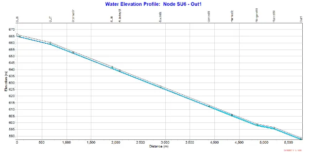
Figure 27: The water elevation profile from beginning to end of the model

showing water depth at the end of the simulation time. ... 67

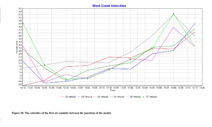
Figure 28: The velocities of the first six conduits between the junctions of the

(13)

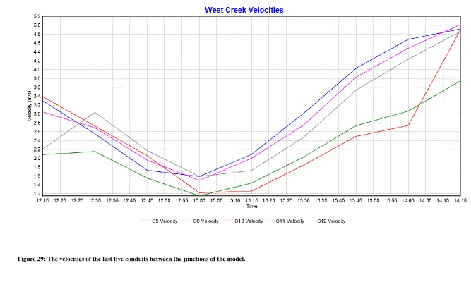
0061019385 xii Figure 29: The velocities of the last five conduits between the junctions of the

model. ... 70

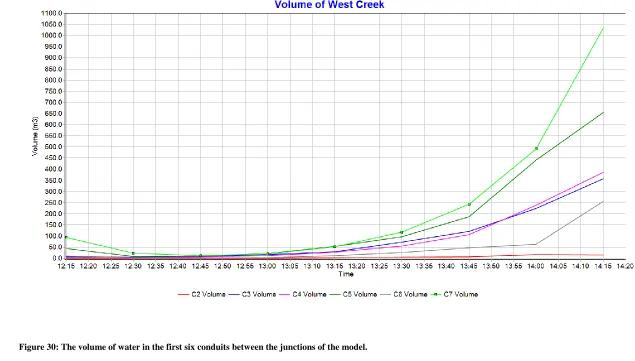
Figure 30: The volume of water in the first six conduits between the junctions

of the model. ... 73

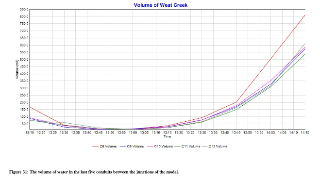
Figure 31: The volume of water in the last five conduits between the junctions

of the model. ... 74

Figure 32: The timeline for the project covering both semesters... 94

Figure 33: A detention basin located along West Creek in between Spring

Street and Stenner Street taken in August 2014. ... 115

Figure 34: A major power line running along West Creek with the power pole

situated directly next to the creek taken in August 2014. ... 116

Figure 35: Concrete footpaths built along West Creek for recreational use

affecting the natural flow of the creek taken in August 2014. ... 117

Figure 36: A toilet block built within the catchment of West Creek used for

recreational purposes taken in August 2014. ... 118

Figure 37: A public shade structure and barbeque built next to West Creek

near Stenner Street taken in August 2014. ... 118

Figure 38: Housing built approximately 30 metres from West Creek affecting

the natural flow of the water into the catchment and in danger of flooding

(14)

0061019385 xiii Figure 39: The piped drainage system used under the Spring Street road

crossing funnelling the water in and out again taken in August 2014.

... 119

Figure 40: An example of the types of tress situated along West Creek taken

in August 2014. ... 120

Figure 41: An example of some of the shrubbery along West Creek taken in

August 2014. ... 120

Figure 42: The results of the Arc Hydro analysis on the 2 m DEM showing

the stream, catchment and drainage points utilising the minimum

threshold... 122

the stream, catchment and drainage points utilising a threshold of 0.3.

... 123

... 124

... 125

(15)

0061019385 xiv Figure 47: The results of the Arc Hydro analysis on the 5 m DEM showing

the stream, catchment and drainage points utilising the minimum

threshold... 127

... 128

... 129

the stream, catchment and drainage points utilising a threshold of 1. 130

Figure 51: The Gowrie creek catchment showing the area which was affected

by rainfall categorised at Q>100 intensity and the location of the rain

gages (ICA, 2011). ... 132

Figure 52: The rain gage files utilised within the hydrological model showing

the amount of rainfall every 15 minutes. ... 133

Figure 53: The parameters utilised in each of the sub catchments within the

hydrological model. ... 134

Figure 54: The summary report generated by the software SWMM after

(16)

0061019385 xv Figure 55: The flow rate of water in the first six conduits between the

junctions of the model... 137

Figure 56: The flow rate of water in the last five conduits between the

(17)

0061019385 xvi

List of Tables

Table 1: The applications defined by the participants of the workshop and the

accuracies required (Apan et al., 2008). ... 17

Table 2: The Meta data of the survey completed for the Toowoomba Regional

(18)

0061019385 1

Chapter 1 Introduction

1.1 Introduction

Living in Queensland presents many risks and dangers when it comes to

weather. One of these risks that can affect nearly everyone in some way is

flash flooding. Flash flooding is the result of a sudden and unexpected amount

of intense rainfall falling over a small area, generally with steep terrain in a

short period of time (ICA, 2011). However living approximately 700 metres

above sea level in the city of Toowoomba would allow complacency when it

comes to flooding. Yet on Monday, 10 January 2011 a 1 in 100 year storm

cell quickly developed over the city dumping intensive rain in a short period

of time over the Gowrie Creek catchment area (ICA, 2011). This in

combination with long term drenching rain that had been previously falling

in the weeks leading up to the event, lead to one of the most devastating floods

in recent time (ICA, 2011).

The Gowrie Creek catchment is a combination of Gowrie, East, West and

Black Gully Creeks. East and West Creeks contain much of the cities

rainwater catchment and converge just before the central business district

(CBD). The catchment is heavily urbanised with multiple manmade features

located within and along the waters flow path.

The intense rainfall that occurred over only a few short hours created flash

flooding that caused damage throughout the creeks and destroyed the CBD

(19)

0061019385 2 dollars worth of damage occurred to the infrastructure within the central

business district. The floodwaters then went down the Toowoomba Range

and hit the un-expecting town of Grantham, where the entire town sustained

heavy damage and more lives were lost. The floodwaters then continued

down the system to join with other floodwaters in the Brisbane River before

leaving to sea (SKM, 2011). An efficient and accurate flooding mitigation

system would have reduced the severity of what was lost within this event,

and any other flooding event. Figure 1 highlights the type of water that was

flowing through the central business district of Toowoomba causing loss of

life and infrastructure damage.

Figure 1: The floodwaters running through the Toowoomba central business district on the afternoon of the flash flooding event (Cook, Frew & Wen, 2011).

In this case the flooding occurred so rapidly that the warning systems were

[image:19.595.114.491.370.623.2]

(20)

0061019385 3 like this flood mitigation requires implementation before an extreme event

such as this is to occur. This would reduce the severity of the flood giving

people more time to prepare, saving money and lives (ICA, 2011). To perform

such a task highly accurate spatial data on the catchment area is vital for the

mitigation of such events (SKM, 2011). Spatial data of such accuracy and size

cannot be collected by traditional survey methods, instead requiring a

different modern type of surveying.

Airborne Light Detection and Ranging (LiDAR) is a rapidly developing piece

of technology that can collect large amounts of spatial data in a short period

of time (Sangster, 2002). This data can be collected faster than traditional

surveying methods whilst still providing accurate results (Kraus and Pfeifer,

1998). The collection of such dense spatial data in a short period of time

allows the generation of high-resolution Digital Elevation Models (DEM).

The DEM is a useful spatial data output that can be utilised in several types

of analysis. Some of these analysis methods include flood plain mapping,

characteristic analysis and hydrological modelling. The DEM can be utilised

within software packages such as ArcGIS and other modelling software

packages for characteristic analysis and modelling (Coleman et al., 2002;

Sithole and Vosselman, 2003). These software tools allow for analysis that

can be used in future flood forecasting and mitigation, which may save lives

and millions of dollars’ worth of damages. This project looks to utilise the

airborne LiDAR data to generate a high quality DEM for a characteristic

(21)

0061019385 4 hydrological modelling making judgements on the catchments capabilities to

deal with rainfall events.

1.2 Research Aim and Objectives

The aim of this project is to utilise LiDAR data to generate a high quality

DEM for characteristic analysis of the West Creek catchment and

hydrological modelling to assist in future flash flood mitigation. Within this

research topic there are multiple objectives based on this aim.

1.2.1 Objective 1

Identify information and methods related to Airborne LiDAR data,

hydrological analysis, modelling and flood plain mapping.

There is a broad range of information on LiDAR data including its history,

data types, collection methods and possible uses. Each of these needs to be

analysed to ensure there is a broad understanding of the topic, with an

emphasis on the hydrological applications of the data. A broad understanding

will allow correct and in-depth analysis in the later stages of the project.

Therefore it is an objective of this project to gain as much information and

knowledge as possible on LiDAR data and its application to waterways.

1.2.2 Objective 2:

Create a Digital Elevation Model.

In order to perform characteristic and hydrological analysis on the LiDAR

(22)

0061019385 5 producing such a map will be required. Once the map is generated a

characteristic analysis can be performed highlighting any areas of interest.

1.2.3 Objective 3:

Utilise the Digital Elevation Model in Hydrological Analysis.

Once the DEM is created hydrological analysis can be performed and a flood

plain map generated. The use of appropriate software such as Arc GIS will

allow a hydrological analysis of the mapped plain. This objective will lead

towards the final goal of identifying areas that require flood mitigation.

1.2.4 Objective 4:

Perform Hydrological Modelling

To further strengthen the analysis and provide more useful information

hydrological modelling is to be completed. Through the use of appropriate

software information such as expected flow rates, velocities and volumes may

be generated when incorporating appropriate meteorological data. This will

help highlight any areas of interest that may not be highlighted in other

analysis.

1.2.5 Objective 5:

Analyse results to determine areas requiring flood mitigation.

Once all of the mapping and modelling is completed all of the collected data

requires analysis. This analysis will aim to determine characteristics or

(23)

0061019385 6

1.3 Justification

This project has many benefits that may arise from its completion. The first

and foremost benefit of utilising airborne LiDAR data for flood plain

mapping, analysis and hydrological modelling is flood mitigation. Flooding

in Australia affects nearly everyone in some form and its mitigation to reduce

damage and save lives is of utmost importance. Having the information and

techniques available to take a proactive approach to mitigation is extremely

important in future work. This project will also help highlight the capabilities

of airborne LiDAR data and its appropriate software. Highlighting its

application to such an important task will help promote airborne LiDAR data

as a high quality and useful survey technology and technique.

1.4 Dissertation Overview

This dissertation contains multiple chapters relevant to the work completed.

There are five main chapters in total and each is given a brief overview below.

Chapter 1 Introduction - This chapter gives an introduction to the topic.

There is background information relevant to the project being undertaken

with the need for the project highlighted. This chapter also states the aim and

objectives of the project to be met throughout.

Chapter 2 Literature Review – This chapter goes over relevant literature to

the project. It covers airborne LiDAR, DEMs, and hydrological modelling.

Chapter 3 Methodology – This chapter highlights the methods utilised to

(24)

0061019385 7 area, the data collection, the generation of the DEMs, the characteristic

analysis and the hydrological modelling.

Chapter 4 Results and Discussion – This chapter highlights the results of

the methodology. It also goes into detail about each of the results and their

relevance to the objectives of the project.

Chapter 5 Conclusions – This chapter concludes the project summing up all

of the information found and makes recommendations for the future.

There is also an extra chapter at the end which contains multiple appendices

relevant to the information within the dissertation.

1.5 Conclusion

This chapter has provided an extensive background into the project. It has

highlighted flooding as a common occurrence within Australia and that it

needs to be dealt with proactively. Through the use of LiDAR data, analysis

can be completed on the catchment to obtain any important information

regarding its hydrological behaviour. Mitigation may then be implemented to

ensure that such an event does not happen again in the future. The justification

of completing this project has been described with mitigation highlighted as

the key outcome. The objectives of the project have also been detailed and

the dissertation outline has been provided. The following chapter will detail

(25)

0061019385 8

Chapter 2 Literature Review

2.1 Introduction

To gain a full understanding on all of the information related to this topic and

the objectives stated in the previous chapter, a literature review was

completed. Several areas were identified as key to the topic and were

thoroughly researched. These areas are airborne LiDAR, DEMs, and

hydrological modelling. This review looks to give an extensive insight into

each of these key areas reviewing previous research and studies.

2.2 Airborne LiDAR

Airborne Light Detecting and Ranging (LiDAR) also referred to as LiDAR,

Laser Altimetry or Airborne Laser Scanning (ALS) is an active remote

sensing technique originally designed to measure the topography of the

earth’s surface (Hollaus, Kraus & Wagner, 2005).

2.2.1 Airborne LiDAR History

The history of LiDAR is extensive with the technologies involved being

studied for an extended period of time. Flood (2001) states that LiDAR data

and the technologies involved around it have been studied since the 1960s.

For multiple years to come there were multiple experiments involving the

advancement of the laser and its usage. Multiple results were returned, both

positive and negative. The first major advancement occurred in the 1980s

when research and design of Airborne LiDAR for topographic data collection

(26)

0061019385 9 et al. (1991) who both reviewed the advancements in the technology at their

time of arrival. This research and design then came into fruition in the 1990s

when commercial LiDAR systems became operational and available for any

surveyor wishing to utilise them, at a high price. Since then LiDAR has come

to the forefront of surveying technology becoming a recognised and well used

method of geographical data collection. This type of technology and its many

uses is an area that will continue to be active in research and development in

the future (Pfeifer and Briese, 2007; Flood, 2001).

Many of the improvements with LiDAR in the modern age involve the

sensors, data processing aspects, increased accuracy, a wider spectrum range

and extraction of object properties (Pfeifer and Briese, 2007). One of the

major modern advances in the technology revolves around the continued

improvement of the laser pulse repetition rate. Flood (2001) states that the

maximum pulse repetition rate previously available for commercial systems

was 50 kHz. However Lemmens (2007) who compared multiple Airborne

LiDAR systems only six years later states that the maximum repetition rate

for commercial systems was around or even higher than 250 kHz. Now seven

years later again there are commercial systems available with repetition rates

above 500 kHz for commercial use (Leica, 2014). This dramatic improvement

in a short period of time shows that LiDAR has and will continue to improve

as more modern technology continues to be developed, providing access to

fast, cheap and dense spatial data. These advances in technology have

presented many modern applications for LiDAR data including hydrological

(27)

0061019385 10

2.2.2 Airborne LiDAR System

An airborne LiDAR system is typically composed of three main components

that work together to collect the spatial data. These three components are the

laser scanner, the Global Positioning System (GPS) receiver and the Inertial

Measurement Unit (IMU) (Hollaus, Kraus & Wagner, 2005; Pfeifer & Briese,

2007). Figure 2 shows how the systems work together along with the aircraft

to collect spatial data. The laser scanner consists of a pulse generator and a

receiver to gather the information of the reflected pulses from the terrain. The

laser works by emitting short infrared pulses towards the earth’s surface.

These pulses can be sent at rates of up to 500 kHz in modern systems with a

faster pulse generation rate resulting in more data in a shorter period of time

(Leica, 2014). A photodiode within the scanner then measures the backscatter

echoes from the pulse generator. The echoes received by the photodiode are

dependent on the objects within the travel path of the laser pulse. The distance

between sensor and the object that it meets can then be determined by

multiplying the time it took for the light to transmit and return by the speed

of light (Watkins, 2005). Therefore laser scanners measure the round trip of

multiple echoes from one laser pulse generated from the scanner (Hollaus,

Kraus & Wagner, 2005; Pfeifer & Briese, 2007). An airborne LiDAR survey

requires the knowledge of where the plane is, so the GPS receiver is used to

record the aircrafts trajectory. The receiver in conjunction with a base receiver

on a known position gives a real time position of the plane as it flies. In

general flight, aircrafts do not stay straight and level, so the IMU unit within

(28)

0061019385 11 possible directions depending on conditions including roll, pitch and yaw.

The IMU measures the roll, pitch and yaw of the plane to allow adjustments

to the collected data if necessary (Dias & Webster, 2006). Each of these types

of plane movement is highlighted in figure 2.

Figure 2: An Airborne LiDAR system highlighting the scanner, GPS and IMU unit (Ohio Department of Transportation, 2014).

2.2.3 Airborne LiDAR Accuracy

The accuracy of the LiDAR data collected is reliant on the accuracy

capabilities of the GPS and IMU units. According to BC-CARNS (2006)

airborne GPS units are capable of accuracies of approximately 5 cm

horizontally and 10 cm vertically. It also states that the IMU units are capable

[image:28.595.113.383.207.509.2]

(29)

0061019385 12 be able to achieve accuracies of approximately 15 cm root mean square

(RMSE) in vertical and 20 cm RMSE in horizontal. This accuracy over a mass

scale in dense data is more than enough for the purpose of flood plain

mapping and analysis. These accuracies are beneficial for many surveying

applications and can be best represented in a DEM.

2.2 Digital Elevation Models

Airborne LiDAR data has multiple possible uses throughout the surveying

world. However the main use for the technology in modern surveying is

spatial analysis. There has been a significant increase in the use of LiDAR

data for DEM generation as more reliable and accurate LiDAR systems are

developed (Sithole and Vosselman, 2003).

2.2.1 Data Source for Digital Elevation Models

Within the surveying profession there are several different ways to collect

spatial data depending on the requirement of the client. Traditional survey

methods of terrain data collection such as field surveying using total station,

GPS and photogrammetry are capable of yielding high accuracy terrain data.

These methods can however be extremely labour and time intensive when it

comes to collecting highly accurate spatial data over a large-scale area. This

extra labour and time makes them inefficient and costly to surveying

businesses, making large-scale spatial data collection difficult. Traditional

methods also provide many data collection issues in areas such as forests

where data cannot be easily collected due to vision problems (Liu, 2008). The

(30)

0061019385 13 can fill in the gap of efficient terrain data collection. Airborne LiDAR can

collect dense data quickly and accurately penetrating through forest areas,

overcoming traditional methods of terrain data collection (Liu, 2008). Kraus

and Pfeifer (1998) demonstrated that this was the case by confirming that

DEMs generated by LiDAR in forests achieved the same accuracy as

photogrammetry in open areas.

Modern LiDAR data capture methods and technology allow for mass

collection of high-density data resulting in an accurate representation of the

earth’s terrain. This however presents other issues with data such as storage

capacity, processing power and manipulation capabilities. Sangster (2002)

highlights that there are several factors, which contribute to the density of the

airborne LiDAR data. These were the pulse rate of the laser, the altitude of

the platform (flying height), the width of the swath, the speed of the aircraft

and the amount of overlap. Each of these needs to be considered when

collecting spatial data and the effects they may have on the processing stage

after collection.

The study completed by Liu (2008) looks to overcome the issues of storage,

capacity and manipulation of airborne LIDAR data by focusing on LiDAR

data filters, interpolation methods and LiDAR data reduction. The section

important to this study is the LiDAR data reduction and the problems that can

occur with it. The main point deduced from Liu (2008) is that it is crucial to

filter or extract the bare earth points from the LiDAR data. However many of

(31)

0061019385 14 A major advantage of airborne LiDAR data is that it has the capability of

presenting objects in a three-dimensional object space immediately after

collection (Al-Ruzoug et al., 2005). After collection the LiDAR points are

initially represented with latitude, longitude and ellipsoidal height based on

the World Geodetic System 1984 (WGS84) reference ellipsoid. These

coordinates on the ellipsoid can be transformed to a national or regional

coordinate system depending on the required use, accuracy and size of the

survey. If the survey is small and only for limited use, the data can be

converted using a regional datum. However if the data collection area is large

and has beneficial use for the state or country, a national system should be

used. Elevations can also be converted from ellipsoidal heights to orthometric

heights based on a national or regional height datum by using a geoid model.

These heights can then be used within the DEM as terrain heights (Dias &

Webster, 2006; Chandra et al., 2007).

The scanner in an airborne LiDAR survey can measure the backscatter signal

from any surface that the beam makes contact with. These non-ground

surfaces can include man-made objects, vegetation or wildlife that are under

the laser at time of collection (Barber & Shortrudge, 2004; Gesch et al., 2006).

Multiple returns of the one pulse occur when the laser pulse meets a target

that does not completely block the path of the pulse, allowing the remained

of the pulse to continue on to a lower target (Anderson, McGaughey &

Reutebuch, 2005). These non-ground points have multiple applications but as

Liu (2008) highlights the separation of these from the ground points is a vital

(32)

0061019385 15 Another type of data that is collected in an airborne LiDAR survey, which

contributes to the improvement of DEM quality, is the intensity of the

backscatter laser pulse. The backscatter signal is a function of multiple

variables including the laser power, beamwidth, range, atmospheric

transmission and target cross section (Briese et al., 2004). The intensity is

created by the optical signal received at the sensor being converted to an

electrical signal by a photo detector. This electrical signal is then quantised

to a digital number by the system, which is the intensity value. This can then

be interpolated to a geo-referenced intensity image, which can assist in

surface classification of DEM’s (Briese et al., 2004; Han et al., 2002)

2.2.2 Digital Elevation Model Generation and Output

To complete the generation of a flood plain map there are several types of

outputs that may be generated. These outputs include, but are not limited to

topographic surface models, thematic land cover maps and two-dimensional

hydraulic surface flow models (Hollaus, Kraus & Wagner, 2005). The DEM

plays a major role in their production due to the DEMs slope, aspect and

drainage networks all being key parameters. The accuracy of these parameters

within the DEM plays a major role in further modelling (Hollaus, Kraus &

Wagner, 2005).

The study completed by Liu (2008) highlights that the Inverse Distance

Weighted (IDW) interpolation method is a suitable interpreter of high density

LiDAR data. The IDW interpolation method assumes that each collected

(33)

0061019385 16 with dense evenly distributed data but does not work as effectively if the

points are sparse or uneven (Childs, 2004). In Liu, McDougall and Zhang

(2011) they generate a high quality DEM from LiDAR data for characteristic

analysis utilising the IDW interpolation method within ArcGIS 10 software.

Liu (2008) also highlights that to improve efficiency and maintain accuracy

the extraction and inclusion of terrain elements such as break lines with the

DEM is an important step. Finally Liu (2008) also states that the DEM

resolution must match the LiDAR density, be able to reflect the changes over

the terrain surface and represent the terrain features. Each of these is vital in

generating a DEM that is capable of flood modelling.

A study completed by Liu and Zhang (2010) looked into the automated

delineation of drainage networks from high resolution DEMs. The study was

completed as the drainage networks are highlighted as one of the main factors

in flood analysis and prediction. The area used for the study covered the entire

Toowoomba City. The extraction of the drainage networks was completed

utilising the Arc Hydro extension of ArcGIS software. The study highlights

that the use of a threshold within the software is important in providing a

detailed drainage network from the DEM. The choice of threshold was shown

to have a direct influence on the detail of the stream network generation. The

study found that a high resolution DEM can provide a detailed delineation of

the drainage network and the catchment if the correct threshold is chosen.

The aforementioned study was furthered by Liu, McDougall and Zhang

(2011) who completed a characteristic analysis of a flood plain utilising

(34)

0061019385 17 within ArcGIS 10 software was utilised. They further extended on the

software’s use highlighting that it can be utilised to perform several forms of

analysis after performing multiple steps. The major steps involve sink filling,

identification of the direction of flow, determination of the flow accumulation

and definition of the stream. It concluded that many different outputs are

available for flood modelling from LiDAR generated DEMs including

longitudinal profiles, shape indices, and hypsometric curves. Each of these

outputs is beneficial in flood plain analysis and will be of use in this study.

2.2.3 DEM Accuracy

Apan et al. (2008) completed a study on the accuracy requirements of a DEM

for use with catchment management. To perform this study a catchment area

over the Condamine River was utilised to generate a DEM from airborne

LiDAR data. The broad requirements and key needs for a catchment DEM

from both an operational and strategic perspective were determined through

the use of a workshop. There were eighteen participants in the workshop who

represented multiple different stakeholders within Queensland. The result of

this workshop can be seen in table 1.

(35)

0061019385 18 It can be seen in table 1 that the areas relevant to this study are the

hydrological modelling, Disaster planning and management (flood and fire)

and insurance and risk assessment. These areas have a required accuracy of

±1 m, <0.5 m and <0.5 m respectively. This study concluded that to produce

such results extreme care has to be taken when collecting the LiDAR data to

generate the DEM. The methods utilised to reduce it are also critical ensuring

that the ground points are accurately represented in the model.

2.3 Hydrological Modelling

As modern technology continues to improve there are always improvements

in software that make once difficult tasks, far easier. Much can be said about

this in the area of hydrological modelling with the development of many

software packages capable of modelling floodwaters. To perform

(36)

0061019385 19 (Elliot and Trowsdale, 2006). The accuracy of the inputted data is vital for

the overall accuracy of the model. Hollaus et al. (2005) performed an analysis

of airborne LiDAR and its usefulness for hydrological modelling. The study

utilised an object based land cover classification to perform the analysis. It

was found that the accuracy of the DEM is crucial in minimising the

uncertainties that can result in flood modelling.

2.3.1 Hydrological Modelling Software

Elliot and Trowsdale (2006) performed a comparison of multiple urban

stormwater management software’s. They completed this study by comparing

multiple software’s against identified attributes including intended use,

temporal use and scale, catchment and drainage network representation,

runoff generation, contaminants in the models, devices and technologies

included, user interface and cost. The three most important attributes to this

study are the catchment and drainage network representation, runoff

generation and cost. The study found that the Model for Urban Stormwater

Improvement Conceptualisation (MUSIC), MOUSE, Storm Water

Management Model (SWMM) and P8-UCM were best when representing a

catchment and drainage network. Each software utilising a spatially

distributed link-node drainage network causes this. This works by

representing each element within the catchment as a node and connecting

them together. Each node can then have flow control devices or treatments

placed on them to give a true representation of how they are in the field. This

study also found that MOUSE, SWMM and MUSIC were greater at

(37)

0061019385 20 initial and continuing loss (MOUSE) and a Green-Ampt infiltration

(SWMM). It is highlighted that there is no one method that is better than any

of the others when generating runoff which each being beneficial to the

modelling. Finally the study showed that of the three mentioned software

models SWMM is the only one that is available free for download and use.

From this study it can be seen that MOUSE, SWMM and MUSIC are three

software models that are quite capable of being used for the hydrological

modelling of a stormwater management system. However due to availability

MUSIC and SWMM will be the two software models researched and

compared.

2.3.2 MUSIC and SWMM

Coleman et al. (2002) identify MUSIC as a powerful modelling tool. The

software was created as many designers were designing stormwater

management strategies ineffectively trying to achieve cost effective

outcomes. Coleman et al. (2002) highlights multiple capabilities of MUSIC

including:

- Determining the water quality from specific catchments.

- Predicting the performance of specific stormwater treatment

measures.

- Designing integrated stormwater management plans for each

catchment.

(38)

0061019385 21 It is noted that MUSIC is a tool to be used as decision support and not as

design software. The software’s main use lies in testing stormwater

management techniques, not designing them (Coleman et al., 2002). Coleman

et al. (2002) highlights that MUSIC utilises the algorithm developed by

Chiew et al. (1997). This algorithm works off the concept that stormwater

runoff is generated from impervious surfaces. The model is based on the

definition of the impervious area and the two moisture storages (deep and

shallow) highlighted in figure 3.

Figure 3: The model adopted within MUSIC for modelling catchment hydrology (Chiew et al., 1997).

There are several stormwater treatment nodes within the both software’s as

(39)

0061019385 22 correct use of each of these treatment nodes is vital in the modelling process.

Both SWMM and MUSIC use treatment nodes such as these in their treatment

train when developing a drainage network (Peterson & Wicks, 2006).

Dickinson and Huber (1992) defined SWMM as a numerical model software

obtainable from the Environmental Protection Agency. The software is

designed for the simulation of flow quality and quantity of urban runoff. As

a result the quality and quantity are a representation of the urban stormwater

runoff and sewer overflow phenomena.

Peterson & Wicks (2006) completed a study into the importance of conduit

geometry and physical parameters utilising SWMM as the software. Within

this study there was a comparison of SWMM to other modelling techniques.

It was deduced that in the studies case, it was good software for the

application and it provided valuable information about the local flow of the

system. This is extremely beneficial to the requirements of this project.

This information shows that both SWMM and MUSIC are both similar

software packages which are suitable for the modelling of urban stormwater.

2.3.3 Meteorological Data

The selection of appropriate rainfall data is a vital step in any sort of

hydrological modelling. The intensity-frequency-duration (IFD) is the

commonly used tool when performing rainfall analysis (Koutsoyiannis,

Kozonis & Manetas, 1998). It can take the form of Q1, Q5, Q10, Q20, Q50

and Q100 depending on the scale of the rain event. A Q1 event is common

(40)

0061019385 23 (Bureau of Meteorology, 2014). This data is available from the Bureau of

Meteorology (2013) who has recently updated all of their IFD data to provide

more accurate rainfall data. Normal rainfall data showing the amount of

rainfall that fell in a certain area can also be obtained from the Bureau if

required.

2.4 Conclusion

This chapter has provided an extensive insight into the literature available

regarding important aspects of this project and its objectives. The chapter has

gone into detail about airborne LiDAR including its history, systems and

accuracy capabilities. The data collected from these airborne surveys was

then discussed and its capabilities to be used in DEMs shown. The use of the

DEMs for characteristic analysis was also highlighted with examples of other

research using similar techniques shown. Finally some of the available

hydrological software packages available including SWMM and MUSIC

were shown, broken down and compared. The application of meteorological

data within these hydrological modelling software packages was also

emphasised. The information and knowledge gained from the research

undertaken in this chapter will now be applied. This will be shown in the

methodology undertaken to meet the objectives of the project in the following

(41)

0061019385 24

Chapter 3 Methodology

3.1 Introduction

After gaining a large amount of theoretical information and analysing past

works, a methodology had to be determined to meet the objectives. A study

area had to be selected and LiDAR data over the study area required

collection. After the data had been collected a DEM was generated from the

ground points of the study area. Slope analysis was then performed on the

DEM to highlight any areas of interest within the study area and to deduce

the flood plain. Hydrological processing was also completed to identify

catchments and streams within the area. Hydrological modelling was then

performed utilising SWMM to highlight areas where mitigation may be

implemented around the catchment and stream network.

3.2 Study Area

3.2.1 West Creek Location

The study area is West Creek, which forms part of the Gowrie Creek

catchment. West Creek starts within southern Toowoomba, running north

through Toowoomba meeting with East Creek near the CBD. The two creeks

then merge to become one creek carrying on through Toowoomba in a

northern direction. The layout of the creeks within the Gowrie Creek

(42)

0061019385 25

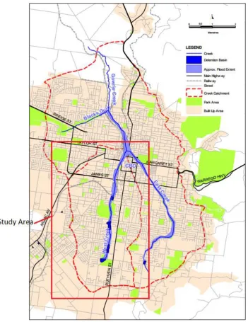
Figure 4: The location of the Gowrie Creek catchment within Queensland (left) and the approximate locations of the creeks within Toowoomba (right) (Liu, McDougall & Zhang, 2011).

West Creek played a major role in the floods that occurred in 2011 and is

therefore an area of major interest (SKM, 2011). It is the largest creek within

the catchment containing an area of water of approximately 16.2 km2 (ICA,

2011). This makes it one of the most important catchments when it comes to

determining a flood plain.

3.2.2 West Creek Urbanisation

All of the creeks within the Gowrie Creek catchment, including West Creek

have been subject to heavy urbanisation due to constant expanding of

Toowoomba (ICA, 2011). This has resulted in structures such as bridge

crossings and housing right up to the edge of the creek, affecting the

catchment. These bridge crossings restrict the flow of the water by funnelling

(43)

0061019385 26 debris. An example of a bridge crossing can be seen in figure 5. Refer to

Appendix E for other pictures related to the urbanisation of West Creek.

These pictures are being used as a representation of the urbanisation and may

not be a 100 % accurate representation of what West Creek was like in

January 2011 before the flooding event occurred.

Figure 5: The bridge crossing over West Creek along Stenner Street in South Toowoomba as of August 2014.

West Creek has been heavily modified with the inclusion of concrete lined

channels, detention basins, piped drainage systems and various other

structures to manage stormwater. These have been included to help manage

the damage around the bridges running over the creek. Other man-made

structures such as concrete footpaths, shade structures and recreational

structures have also been recently included for the use of the public. These

(44)

0061019385 27 different surface for it to run over and altering its path. An example of

concrete lining being used in West Creek can be seen in figure 6.

Figure 6: Concrete lining on the lowest part of West Creek in between Spring Street and Stenner Street in South Toowoomba as of August 2104.

West Creek also contains a combination of varying grass types, shrubs and

trees at moderate grade changes. The trees and shrubs within the catchment

(45)

0061019385 28 the catchment has a strong effect on the water the water flows within the

catchment. It can help slow the flow of water and hold the ground together.

However these trees and shrub can also become debris to block the pipe ways

and road crossings. An example of the type of nature within West Creek can

be seen in figure 7.

Figure 7: The types of trees and shrubbery along West Creek as of August 2014.

This study area is an excellent example of a watercourse located within an

urbanised area that contains many varying factors including ground cover,

trees, grade and manmade features. Each of these factors contributes and

affects the way the water flows and meets with the rest of the catchment

further downstream.

The study area, particularly near the CBD has undergone heavy man-made

(46)

0061019385 29 Regional Council for their flood mitigation program. Due to this the creek is

not as it was in some areas when the data was collected at the end of 2010.

However for the purpose of this research project West Creek will be treated

as close as possible to how it was in 2010.

3.3 Airborne LiDAR Data

3.3.1 Data Collection

It was decided that collecting new LiDAR data would be majorly time

consuming and too expensive for the purpose of this project. Also as the

flooding event occurred over four years ago, new data over West Creek would

not be a good representation of the flood plain. Instead LiDAR data was found

of the Toowoomba area from another source.

The LiDAR data was sourced from the Toowoomba Regional Council who

had Schlencker Mapping Pty Ltd conduct a Toowoomba wide airborne

LiDAR survey covering 2760 km in 2010. The data collection was undertaken

utilising an ALTM Gemini ALS scanner on a fixed wing aircraft. The Meta

data for the LiDAR survey can be seen in table 2 below. The entire report can

(47)

0061019385 30

Table 2: The Meta data of the survey completed for the Toowoomba Regional Council (Schlencker Mapping Pty Ltd, 2010).

It can be seen from table 2 that the survey was completed late June and early

July placing it approximately six months before the flooding event occurred.

The plane flew at a height of 1200 m completing two hundred and forty two

runs in total. The swath width of the laser scanner was 1000 m and there was

a 30 % overlap for the survey. Of note within the Meta data is the average

point separation, which is 1 m. This shows that the LiDAR data collected is

of extremely high density allowing greater accuracy. The metadata also

shows that the horizontal accuracy of the data is 0.15 m and the vertical

accuracy is 0.22 m, both at the first standard deviation. These accuracies are

within an expected range for an airborne LiDAR survey making the data

suitable for analysis (BC-CARNS, 2006).

3.3.2 Data Validation

The same surveying company, through the use of a vehicle mounted GPS

(48)

0061019385 31 GNSS receivers collecting data at 50 m intervals. The survey covered a total

of 218 km along bitumen and gravel roads collecting six thousand three

hundred and thirty two points at an accuracy of ± 0.05 m. This GPS survey

highlighted that 94 % of the LiDAR points collected are within 0.15 m of

their true points.

The data provided had the ground points and non-ground points already

separated in a binary LAS file format. There was no mention of the technique

utilised to separate the ground and non-ground points.

3.4 Digital Elevation Model Generation

The generation of the DEM required the use of ArcGIS 10.2 software. Liu

(2008) highlights that one of the most critical aspects of DEM generation with

LiDAR data is the separation of ground and non-ground points. However in

this case the LiDAR data had been provided already separated, taking out this

step of the process. Thirty-five text files were utilised which were each

approximately 1 km2_{in size. These files stretched far enough to give an}

accurate representation of the catchment area.

3.4.1 Inverse Distance Weighted Interpolation Technique

The generation of the DEM could be completed utilising multiple different

tools. In the study completed by Liu, McDougall and Zhang (2011) the DEM

was generated by the IDW interpolation technique. The technique is

mathematical that uses a linearly weighted combination of points to determine

(49)

0061019385 32 mapped decreases as its distance from the sample location grows (Phillip &

Watson, 1985). This is highlighted in figure 8.

Figure 8: The Inverse Distance Weighted sample location used when processing the points whilst generating a DEM (ESRI(a), 2014).

The range of values used to interpolate limits the output of a cell using this

technique. Due to the results being a weighted distance average, sudden rises

or falls cannot be generated unless they already have data collected over them.

To get the best results from the method dense data sampling is required, if not

the results may not be a true representation of the surface (Phillip & Watson,

1985). In the case of the data over West Creek there are no sudden rises or

falls with consistent grade changes throughout. The data has also been

densely collected as mentioned in section 3.3.1 at a ground separation

distance of 1 m. As a result the IDW technique would present an accurate

(50)

0061019385 33

3.4.2 Topo to Raster Interpolation Technique

Another technique that may be utilised to generate a DEM is the Topo to

Raster interpolation tool. The Topo to Raster tool is one that has been

designed for the generation of DEMs that are correct in a hydrological sense.

This tool is based on the ANUDEM program, which was developed by

Michael Hutchinson (Hutchinson, 1988). The technique imposes constraints

while it interpolates the elevation values of a raster surface to ensure that the

final outcome has a true representation of drainage, ridges and streams. The

interpolation technique used within this method is an interactive finite

difference technique. It utilises the knowledge of landscapes having multiple

hilltops and minimal sinks to generate a connected drainage pattern. The

drainage conditions that are imposed upon the surface help generate an output

that is best for hydrological work and requires little to no post processing

(ESRI(c), 2014).

A choice had to be made between the two techniques as to which should be

utilised. The Topo to Raster interpolation tool was chosen to generate the

DEM. The IDW tool requires one surface to be input, which can then be

created into a DEM. This means that other tools such as the merge tool would

be required to generate the DEM, increasing the chances of error. Whereas

the Topo to Raster tool allows multiple input files and generates the surface

from each individual input. This technique is also specifically made to

generate DEMs that are hydrologically accurate, making it the clear choice

(51)

0061019385 34 To generate the DEMs the Topo to Raster interpolation technique was

utilised. The text files had to be displayed with the appropriate Map Grid

Australia 1994 (MGA1994) projection. In Toowoomba the correct map grid

correction is zone fifty-six. Each tile once displayed was then exported into a

shape file to allow generation of the DEM.

To generate the DEM the individual shape files were inputted and the output

cell size was set at two. This generated a DEM with a resolution of 2 m. A

second DEM was also generated with the same input shape files with an

output cell size of five. This allowed for the generation of a DEM with a

resolution of 5 m. The two different resolutions were chosen to observe the

differences in the generation of the stream networks and catchment size in

later modelling.

3.5 Hydrological Analysis

Once the DEMs were generated the hydrological analysis was completed. The

initial steps of the analysis were completed in Arc Hydro to perform

hydrological analysis of the catchments and drains. Following the

hydrological analysis a slope map was generated to determine the flood plain.

Liu, McDougall and Zhang (2011) and Liu & Zhang (2010) completed a

characteristic analysis and extracted drainage networks from DEMs

previously. Both studies showed that that the extraction of drainage networks

is based on the widely used D8 algorithm. Within this algorithm the correct

choice of threshold values is vital to the accuracy of the stream network. To

(52)

0061019385 35 ArcGIS 10.2 software was utilised. This extension of the software can be

utilised to perform several forms of analysis after performing multiple steps.

3.5.1 Arc Hydro Pre Processing

The steps involved in the pre-processing for Arc Hydro are extremely

important and must be completed in the correct order for the processing to

work. The first step involves reconditioning the DEM by imposing linear

features onto it. This step is an optional one and does not need to be

completed. The second step involves filling all of the sinks within the DEM.

If there is a cell in the DEM that has multiple high cells around it, the water

will not flow causing issues in the modelling. This step fills those cells to

ensure that this does not occur (ESRI, 2011).

Once filled the direction of flow for each cell is determined from the steepest

descent values within the cells. The next step involves determining the flow

accumulation. The flow accumulation creates a grid showing the number of

cells, upstream of a cell. Following the flow accumulation the stream must

then be defined. Within this step there is a stream threshold that must be input.

It originally displays 1 % of the maximum flow accumulation, but this may

be changed. The result is a grid that shows all of the cells from the input flow

accumulation that has a value greater than the threshold entered (ESRI, 2011).

The next step is stream segmentation where each steam is given a unique

identifier. Following the segmentation the catchment grid delineation is

created. This step creates a grid where each cell carries a value that is an

(53)

0061019385 36 steps may be completed to generate the polygon lines for the stream and the

catchment, making a better representation. The adjoining catchments can also

be generated which show any catchment that is not a head catchment. Finally

the drainage points can be generated which shows the point where water

would be expected to drain from each stream. Once these have been

determined further analysis can be completed including determination of

surface area, shape indices and the creek profile (ESRI, 2011).

The Arc Hydro pre-processing analysis was completed on both the 2 m DEM

and the 5 m DEM. The pre-processing for each of the DEMs followed the

same steps except for the input of the threshold value in the stream definition

step. The 2 m DEM had thresholds of 0.1970 that is the minimum 1 %, 0.3,

0.5, 0.75 and 1. Each of these and the corresponding number of cells can be

(54)

0061019385 37

Figure 9: The multiple inputs for each of the stream definitions during pre-processing of the 2 m DEM.

The same process was followed with the 5 m DEM. The threshold inputs for

the 5 m DEM were 0.1975 which was the minimum 1 %, 0.3, 0.5, 0.7 and 1.

The threshold inputs and their corresponding number of cells can be seen in

(55)

0061019385 38

Figure 10: The multiple inputs for each of the stream definitions during pre-processing of the 5 m DEM.

Once the streams and catchments were generated analysis was completed on

each of the maps to identify the stream networks and the size and shape of the

(56)

0061019385 39

3.5.2 Slope Analysis

The slope tool works by identifying the gradient or rate of maximum change

in the z value of each individual cell compared to its neighbours. The steepest

downhill descent for the cell is then determined by finding the maximum

change in elevation between the eight surrounding cells and the cell itself. If

there is no data within a cell then it is left as having no data within it

(Burrough & McDonnell, 1998). An example of how the cells works can be

seen in figure 11.

Figure 11: The way the cells are worked within a slope analysis (ESRI(b), 2014).

The generation of the slope analysis surface was completed on the 5 m DEM

created through the Topo to Raster technique. The generation of slope

analysis on both the 2 m and 5 m DEM was deemed meaningless and was not

completed, as the results were almost identical. The surface was generated

with a percentage representation instead of a degree representation. The Z

factor for both slope surfaces was kept as default which was 1. Once

generated the surfaces were reclassified to 0 - 2 %, 2 - 5 %, 5 - 10 %, 10 - 20

(57)

0061019385 40 representation of the slopes within the creek highlighting the areas which may

be the flood plain. The resulting slope map was then analysed with the areas

that fell within the 0 - 2 % and 2 - 5 % deemed a chance of being a flood

plain.

3.6 Hydrological Modelling

To perform the hydrological modelling software had to be chosen. The choice

was between MUSIC and SWMM. It was decided that since both software

packages offer similar analysis, SWMM would be utilised for the analysis.

SWMMs ability for free download and use with online guides and tutorials

compared to MUSICs restrictive access and paid tutorials made it the obvious

choice.

To begin the analysis the treatment train had to be drawn over the study area.

SWMM has multiple different forms of hydrological components that can be

utilised to represent the system on the ground. These components can be

generally broken into nodes or links. Within each of these, the main

LiDAR data for DEM generation and flood plain mapping

University of Southern Queensland