Tectono-metamorphic evolution of the high-temperature low-pressure (HTLP) Cooma Metamorphic Complex, Lachlan Fold Belt, S. E. Australia
303
0
0
Full text
(2) TECTONO-‐METAMORPHIC EVOLUTION OF THE HIGH-‐TEMPERATURE LOW-‐PRESSURE (HTLP) COOMA METAMORPHIC COMPLEX, LACHLAN FOLD BELT, S. E. AUSTRALIA . Mark A. Munro. Submitted July 2013 for the degree of Doctor of Philosophy, James Cook University..
(3) STATEMENT OF CONTRIBUTION FROM OTHERS:. I am grateful for the editorial assistance received from Simon Richards, Tim Bell, Tom Blenkinsop and Carl Spandler throughout the duration of my candidacy. The wealth of experience and enthusiasm shared with me by these people during my research will prove invaluable in my future endeavours. $500 conference support was received from the School of Environmental Sciences.. $200 student conference support was also received from Geoscience. Australia to attend the 2010 Port Macquarie SGTSG conference. $500 was provided by the Economic Geology Research Unit to attend the Waratah SGTSG conference in January 2012. The Geoscience Australia SGGMP also provided $500 to attend the IGC conference in Brisbane in August 2012. $1000 was received from the School of Earth & Environmental Sciences funding round in 2010. $2000 was also received from the GRS in 2010. $3000 was received in the SEES/GRS funding round 2011. $1800 was also received from the SEES/GRS funding round in 2012. Section A of the thesis is published in Computers & Geosciences, with Tom Blenkinsop as a co-author on the paper.. Munro, M., Blenkinsop, T., 2012. MARD-A Moving Average Rose Diagram application for the Geosciences. Computers & Geosciences 49, 112–120.. Tom helped prepare the final manuscript for publication in the usual manner of a co-author. His contributions to the paper were writing the Microsoft Excel version of the program. I wrote the MATLAB and GNU Octave versions of the program, wrote the paper and prepared the illustrations..
(4) ACKNOWLEDGEMENTS. In addition to the academic staff at James Cook University who were always willing to provide assistance in any way possible, I am grateful to a large number of people who made my time in Queensland such a memorable experience. Upon arrival in Townsville I was immediately made to feel at home by the cosmopolitan environment established by Tim in the Structure and Metamorphism Research Institute (SAMRI). Ioan, Raph, Clem, Jyotindra, Ahmed, Afroz, Chris and Hui – you were a continual source of inspiration as I delved deeper into the world of structural geology. The countless debates held around the table challenged my views and theories, and strengthened my critical thinking.. My gratitude also for. introducing me to the legendary ‘WE 3/WE C’ cleanskin wine at Dan Murphys. Anyone reading who hasn’t tried this – best $3 bottle of red wine on the go. Ioan and Raph, the house in Cranbrook was great banter. Clem, our countless discussions during my final year helped consolidate many of my ideas. Cait, thanks for being incredibly patient throughout the whole process and in particular for cooking for me continually to save time during the final stages. It was certainly demanding, but you managed to keep me sane. Thanks however are not extended for almost incinerating my eyebrows while making sausage rolls! Johannes, Ryan, Rob, Babo, Yanbo, Hannah, Astrid and Emma, cheers for a great laugh up in the corridor, awesome pub crawls and for keeping me in touch with other avenues within geology. I hope everyone’s work goes well and all the best for finishing up! I am also thankful to all the undergrad students who I had the privilege to work with and share many drunken nights. You all made learning to tutor and lecture.
(5) such a rewarding and stress-free experience. The field courses to Fanning River and Cloncurry will always be one of the highlights of my time at JCU. You were such a great bunch, cheers! Glen, Melissa and Bec, thank you for being the best admin staff, always willing to run around like headless chickens to make life so much easier for everyone. In particular, for bending over backwards to ensure my confirmation and precompletion seminars could happen when they needed to, despite major time constraints. Finally, a heartfelt thanks to Mum, Dad, Stu, Granny, George and Alison – the best Skype support team in the Northern hemisphere! I am ever grateful for your enthusiasm, encouragement, ‘red cross packages’ and for keeping me in touch with happenings in the UK. But, perhaps most importantly, for pushing me to fulfill my desire to move to Australia to do this work. Slàinte mhath!. .
(6) THESIS: TABLE OF CONTENTS. STATEMENTS AND ACKNOWLEDGEMENTS VOLUME I - MANUSCRIPTS SECTION A………………………………………………………………………………………p2-27 MARD – A moving average rose diagram application for the geosciences SECTION B………………………………………………………………………………………p28-62 Porphyroblast microstructures: A review of strategies for their observation and measurement SECTION C………………………………………………………………………………………p63-97 Tectono-metamorphic evolution of the Western Cooma Metamorphic Complex, Lachlan Fold Belt, S. E. Australia SECTION D……………………………………………………………………………………p98-135 Tectono-metamorphic histories preserved by the high-temperature low-pressure (HTLP) Cooma Complex and associated Murrumbidgee aureole in the Eastern Lachlan Fold Belt: An intricate record of regional-scale tectonics? SECTION E……………………………………………………………………………………p136-172 Mass transfer associated with differentiated crenulation cleavage and strain shadow development during HTLP metamorphism: Insights from the Cooma Metamorphic Complex, S. E. Australia CONCLUSIONS……………………………………………………………………………….p173-182. VOLUME II – FIGURES & APPENDIX SECTION A……………………………………………………………………………………p183-194 SECTION B……………………………………………………………………………………p195-207 SECTION C…………………………………………………………………………………....p208-228 SECTION D……………………………………………………………………………………p229-243 SECTION E……………………………………………………………………………………p244-272 APPENDIX 1…………………………………………………………………………………..p273-297.
(7) Section A . M. A. Munro . - VOLUME I MANUSCRIPTS. . 1 .
(8) Section A . M. A. Munro . - SECTION A -. MARD – A MOVING AVERAGE ROSE DIAGRAM APPLICATION FOR THE GEOSCIENCES. . 2 .
(9) Section A . M. A. Munro . MARD – A MOVING AVERAGE ROSE DIAGRAM APPLICATION FOR THE GEOSCIENCES. Abstract ......................................................................................................................... 4 1. Introduction .............................................................................................................. 6 2. Moving average rose diagrams: overview and evaluation ................................... 7 2.1 Moving average rose diagrams: a definition ................................................................... 7 2.2 Types of moving average: weighted versus unweighted ................................................. 8 2.3 Weighted moving averages in MARD ............................................................................. 9 2.4 The ‘up-scaling factor’ for weighted moving averages ................................................. 10 2.5 Benefits and Limitations ................................................................................................ 11. 3. Implementing moving average rose diagrams: adjustable parameters ............ 12 3.1 Data type ........................................................................................................................ 13 3.2 Number of datasets to be plotted .................................................................................... 14 3.3 Aperture .......................................................................................................................... 14 3.4 Selecting an appropriate weighting factor ...................................................................... 15 3.5 Equal area option ............................................................................................................ 16. 4. Using MARD .......................................................................................................... 16 4.1 The MATLAB® version ................................................................................................. 17 4.2 The GNU Octave version ............................................................................................... 18 4.3 The Microsoft® Excel version ........................................................................................ 18. 5. Applications ............................................................................................................ 19 5.1 “Uni-directional” option (all versions) ........................................................................... 19 5.2 “Bi-directional” option (all versions) ............................................................................. 20 5.3 “Pitches/plunges” option (MATLAB® & Octave versions only) ................................... 21. . 3 .
(10) Section A . M. A. Munro . 6. Conclusions ............................................................................................................. 22 References ................................................................................................................... 24. . 4 .
(11) Section A . M. A. Munro . ABSTRACT. MARD 1.0 is a computer program for generating smoothed rose diagrams by using a moving average, which is designed for use across the wide range of disciplines encompassed within the Earth Sciences. Available in MATLAB®, Microsoft® Excel and GNU Octave formats, the program is fully compatible with both Microsoft® Windows and Macintosh operating systems. Each version has been implemented in a user-friendly way that requires no prior experience in programming with the software. MARD conducts a moving average smoothing, a form of signal processing low-pass filter, upon the raw circular data according to a set of pre-defined conditions selected by the user. This form of signal processing filter smoothes the angular dataset, emphasising significant circular trends whilst reducing background noise. Customisable parameters include whether the data is uni- or bi-directional, the angular range (or aperture) over which the data is averaged, and whether an unweighted or weighted moving average is to be applied. In addition to the uni- and bi-directional options, the MATLAB® and Octave versions also possess a function for plotting 2dimensional dips/pitches in a single, lower, hemisphere. The rose diagrams from each version are exportable as one of a selection of common graphical formats. Frequently employed statistical measures that determine the vector mean, mean resultant (or length), circular standard deviation and circular variance are also included. MARD’s scope is demonstrated via its application to a variety of datasets within the Earth Sciences.. Keywords:. Rose Diagram, Moving average, Circular statistics, Vector mean,. MATLAB®, Microsoft® Excel. . 5 .
(12) Section A . M. A. Munro . 1. INTRODUCTION. Moving averages, sometimes referred to as running averages, are a form of signal processing filter which produce averages of subsets of data series from within the master data series in 1-dimension. Data filtering of this kind serves a broad variety of applications within science and engineering, being primarily utilised to accentuate trends in data that are otherwise generally less apparent, or to recover meaningful signal components by removing the high-frequency noise. Other uses include 2dimensional enhancements in the resolution of graphics, and providing a form of interpolation that generates intermediate values. Within the Earth Sciences, such analyses are commonly applied in various forms for image processing of aerial photographs, maps and satellite images (Diniz da Costa & Starkey, 2001; Jordan, 2007). Moving averages may be applied to rose diagrams that depict azimuthal data. At present, moving average rose diagrams are not commonly used within the Earth and Environmental Sciences; however, they are a very effective means of visualisation (e.g. Aerden, 2003; 2004; Aerden & Sayab, 2008). The most obvious benefit of this representation is that the commonly segmented, or ‘blocky’ appearance of rose plots, due to aggregation of data in bins, is avoided. This eliminates the artificial stepping at bin margins in conventional plots, and furnishes a more accurate representation of where data lies within each bin. A range of good quality software is available for plotting geoscience data on both Mac and Windows platforms. Within these programs, rose diagrams are a common function. Examples include GEOrient (Holcombe, 1994), Spheristat™, RJS ©. graph, Stereonet , OSXStereonet , Grapher™, KaleidaGraph , Rose.C (Kutty & ©. ©. ©. Ghosh, 1992) and EZ-Rose (Baas, 2000). However, only one of these, Spheristat™,. . 6 .
(13) Section A . M. A. Munro . presents a ‘smoothing’ function for rose and polar diagrams that is similar to a moving average filter. This program is relatively expensive to purchase and is only available for Windows. The primary aim of this paper is to promote the use and benefits of moving average filters within rose diagrams via the provision of freely distributable, userfriendly programs which do not require any prior knowledge of high-level programming languages. Three formats are presented for users to readily produce a moving average rose diagrams on either Windows or Macintosh platforms. MARD is available 1) as a script written for MATLAB®, 2) a script for GNU Octave and 3), a macro implemented for use in conjunction with Microsoft Excel. The benefits of MARD are illustrated via its application to a diverse range of datasets within the Earth and Environmental sciences.. 2. MOVING AVERAGE ROSE DIAGRAMS: OVERVIEW AND EVALUATION. 2.1 Moving average rose diagrams: a definition. When presenting rose diagrams, the most common convention within the Earth Sciences is to represent azimuthal data utilising 10° bins, the frequencies of which represent the sum of all of the azimuths within that bin. Binning is used in order to emphasise major trends in data, but inherently loses a certain level of detail. . 7 .
(14) Section A . M. A. Munro . because the distribution of data within the bins is unknown. Moreover, the arbitrary selection of bin width and boundaries may have a significant impact upon the result. Moving average rose diagrams, on the other hand, evaluate the frequency of each azimuth within the context of those in immediate proximity to it. The frequency of each azimuth, and those of azimuths within a pre-defined range (the aperture, or moving window) either side of it are systematically summed and averaged. The resultant average for each azimuth is then assigned to the central value position and plotted on the final rose diagram. The broader the aperture, the greater the smoothing effect.. 2.2 Types of moving average: weighted versus unweighted. Moving averages may be either unweighted (a.k.a. a ‘simple’ moving average) or weighted. Where no weighting is applied, each azimuth frequency within the aperture is counted as its full value, i.e. each is deemed equally important in determining the local average:. n =α +. Mα =. 1 A. A −1 2. ∑F. i A −1 i=α − 2. (1). where: Mα is the unweighted average value to be subsequently plotted on the rose. €. diagram for that azimuth, α is the azimuth for which the average is determined, Fi is the raw frequency at angle i, A is the aperture size.. . 8 .
(15) Section A . M. A. Munro . Alternatively, when a weighted moving average is applied, the raw values of the data in azimuths outside the central one are reduced by a magnitude that depends upon their proximity to the centre. The raw value of immediately adjacent data is reduced by less than those nearer to the margins of the aperture. Weighting permits more emphasis to be placed upon those data closer to the centre of the aperture. A weighted mean is thus less than, and represents a proportion of, an equivalent unweighted mean. In many applications, especially when dealing with large datasets, unweighted moving averages are appropriate.. However, in a number of circumstances the. application of a weighted average might be more beneficial. One such example is when handling small datasets. In particular, where data is clustered, an unweighted moving average may result in a ‘plateau’ distribution like a binned plot. The use of a weighted moving average in scenarios such as this provides a means of smoothing the data markedly whilst still preserving the local maxima.. 2.3 Weighted moving averages in MARD. In MARD, weight is distributed among the azimuths in a non-linear fashion, because linear methods are intrinsically restrictive: for example, reducing each value progressively by 10% from the central position can only be achieved for 10 positions either side before becoming negative. However, the non-linear method is applicable to any aperture. The user specifies a proportion, expressed as the weighting factor, which reduces the contribution of each neighbouring raw value with increasing distance from the reference position. Thus, in calculating the moving average around an azimuth of 87° using a weighting factor of 0.9, the frequencies of data at azimuths. . 9 .
(16) Section A . M. A. Munro . of 86° and 88° (one position removed from the centre) are reduced to 0.9 of their full values, and the frequencies at azimuths of 85 and 89° (two positions removed) are reduced to a proportion of 0.9 x 0.9 = 0.81 of their full values. The moving average for that azimuth is then the average of these weighted values within the aperture in the same manner as an unweighted average, and is represented as:. 1 Mwα = A. n =α +. A −1 2. ∑F ⋅ w. α−. A −1 2. i A −1 i=α − 2. (2). where: Mwα is the weighted average value to be subsequently plotted on the rose. €. diagram for that azimuth, α is the azimuth for which the average is determined, Fi is the raw frequency at angle i, A is the aperture size, w is the value of weighting factor applied.. 2.4 The ‘up-scaling factor’ for weighted moving averages. One effect of weighting the averages as described above is that it lowers the frequencies of the plot relative to those within an equivalent unweighted plot. The degree to which this occurs is proportional to the degree of weighting applied. Where the adjacent values are still weighted relatively strongly (e.g. a weighting factor of 0.95) then the frequencies will not be reduced to a large degree. On the other hand, if the adjacent values are allocated much lower weight than the central (e.g. 0.7) then the magnitude of frequencies will be reduced considerably more, resulting in a notable loss in magnitude of the moving average.. . 10 .
(17) Section A . M. A. Munro . In order to counter-act this effect, an ‘up-scaling factor’ is applied to the weighted moving average frequencies.. The value of this factor is inversely. proportional to the value of weighting factor selected and is given as:. 1 = 1+ 2 D. n=. A −1 2. ∑w. i. i=1. (3). where: 1/D is the up-scaling factor, A is the aperture size, w is the weighting factor. To upscale the weighted moving average, the proportion of the equivalent unweighted. €. mean that the value of the weighted mean should represent is calculated for the selected aperture size and weighting factor applied. Each weighted frequency is then multiplied (up-scaled) by the inverse of this proportion. This restores the absolute frequencies back into a range equivalent to that of an unweighted moving average, so that they can be compared to the unweighted moving averages.. 2.5 Benefits and Limitations. The primary advantage of moving average rose diagrams over their binned counterparts is the removal of the coarse, blocky appearance of the former, with artificial steps at bin boundaries. The product is a plot that is more visually appealing and notably more informative.. Moreover, the suppression of minor variations by. averaging accentuates significant changes or trends in the data. The main objective of applying moving averages to a dataset is to smooth the plot to emphasise the significant trends present, whilst retaining its original character as much as possible. Filtering data in this way inherently provides more context for the distribution of frequencies around the compass, and within individual bins, than conventional plots.. . 11 .
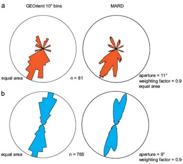
(18) Section A . M. A. Munro . Consequently, moving averages commonly reveal a more accurate representation of the distribution of modal maxima within a dataset than are otherwise portrayed in an equivalent binned counterpart (Fig. 1). One limitation of the moving average method by calculating a mean value (as implemented in MARD) is that it may potentially be influenced by outliers, i.e. spurious maxima. A median average method (e.g. Jordan, 2007) may ameliorate this problem, and this could be implemented in future versions of MARD. At present, however, the mean method is proposed because it is the most common and readily understood type of moving average.. 3. IMPLEMENTING MOVING AVERAGE ROSE DIAGRAMS: ADJUSTABLE PARAMETERS. In the MARD program the user pre-defines a number of parameters; data type (this determines how the data are handled), number of datasets to be plotted, unweighted or weighted averaging, the magnitude of weighting (if applicable), and the sampling aperture (angular window over which the data is to be averaged). The following section addresses the principal considerations associated with each of the above.. . 12 .
(19) Section A . M. A. Munro . 3.1 Data type. MARD handles three types of data. “Uni-directional” is implemented for use with uni-directional data, i.e. vectors that have a unique direction and therefore one compass azimuth only, for example palaeocurrents. “Bi-directional”, is designed for use with bi-directional data, i.e. lines that are specified by one azimuth as well as the complementary one at 180°, for example the strikes of planar features such as bedding or tectonic foliations.. The distinction between uni- and bi-directional data is. sometimes referred to as the difference between directional and oriented data (Davis 2002). The third data type (MATLAB® and Octave versions only) was incorporated primarily for representing porphyroblast inclusion trail pitches, a common application in microstructural geology. For this data type, MARD generates a single semicircle below a diameter that represents an artificial horizontal reference. Data represent the inclination, or pitch, of each element from the horizontal reference plane, with those inclined to the right of the page trending towards a given compass orientation and those to the left towards its complement. A selection of circular statistical functions commonly utilised to evaluate such datasets are also included. These include the vector mean, mean resultant, circular standard deviation and circular variance/dispersion (Fisher, 1993; Davis, 2002; Pewsey, 2004; Allmendinger et al, 2012). These functions are equipped to handle both integer and non-integer values.. A number of fully comprehensive circular. statistics toolboxes are already available for MATLAB® (Jones, 2006; Berens & Velasco, 2009).. The vector statistics capability of MARD is not intended as a. replacement for these, but is incorporated for convenience.. . 13 .
(20) Section A . M. A. Munro . 3.2 Number of datasets to be plotted. The operator specifies the number of datasets they wish to be plotted in the rose diagram (MATLAB® and Octave versions only). Each dataset is then input independently when prompted. Generally it is recommended that no more than three datasets be plotted at once to avoid overpopulating the rose.. 3.3 Aperture. Apertures are designated by odd values, so that the resultant average is positioned in the central location within it. The aperture size exerts first-order control upon the appearance of the resultant moving average plot. The lower the aperture, the closer the plot will resemble the raw, unaveraged, data, plotted in 1° increments. This assumes that the data being dealt with are in integer degree format, however directional data may also be non-integer. If the latter are input, they are automatically rounded to the nearest integer prior to counting. As the aperture is increased, the plot becomes progressively more generalised, i.e. smoother (Fig. 2). The more irregular the original dataset is, the larger the aperture that may be required in order to smooth it. Consequently, the user’s discretion is necessary to decide which aperture is most suitable for any given plot. One convention is to start with the unaveraged plot (1°) and incrementally increase the aperture by 2° until the desired effect is achieved. However, in our experience we have found an aperture of 9° to prove a suitable benchmark.. For some datasets an aperture of as little as 5° may be sufficient,. however others may require a significantly greater value. Some previously published. . 14 .
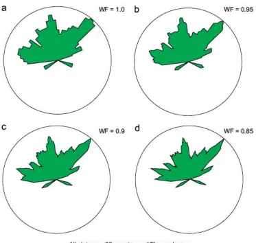
(21) Section A . M. A. Munro . moving average roses (e.g. Aerden, 2003; 2004; Aerden & Sayab, 2008) have utilised apertures of 21°, which have produced appropriate smoothing. It is also important to preserve the essence of the data such that it is still representative of the original and does not become biased or highly distorted. Beyond a certain value of aperture the data will begin to homogenise as apertures are progressively increased, amalgamating the major trends and becoming too generalised (e.g. Fig. 2d). This arises due to the large portions of the data now being averaged, with each aperture averaging essentially the same sub-set. Thus, the aperture utilised is dependent upon what the user wishes to highlight and to what degree they wish to preserve the minor peaks.. 3.4 Selecting an appropriate weighting factor. The largest weighting factor of 1 will return the same values as an unweighted average, whereas a minimum possible factor of 0 will produce a scaled-down version of the original non-averaged dataset. Thus, there is an inherent limit to the value of weighting factor that may be applied to smooth a particular dataset before it begins to resemble the original dataset. For this reason, we recommend using weighting factors between 1.0 and 0.7. These values are sufficient to smooth the data, whilst remaining sufficiently different to the original dataset. It is advisable to begin with a higher weighting factor (e.g. 0.95) and progressively decrease the value in 0.05 increments until the smoothing is sufficient. Values of 0.95 or 0.9 are most commonly adequate. The effects of applying different weighting factors are illustrated in figure 3.. . 15 .
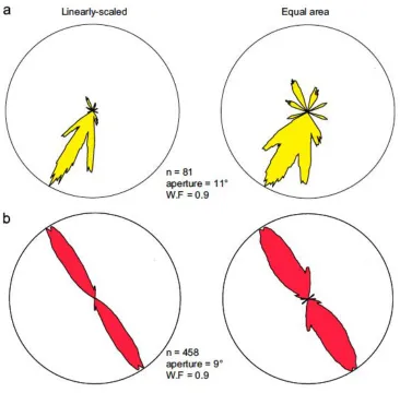
(22) Section A . M. A. Munro . 3.5 Equal area option. Commonly used rose diagrams with a linear radial scale for frequency generate visual bias due to the widening of a petal as it extends outwards from the origin (Nemec, 1988).. Frequencies may appear notably more or less prominent. relative to those surrounding them in a manner disproportionate to their absolute differences in magnitude, potentially promoting mis-interpretations of apparent preferred orientations (Nemec, 1988; Wells, 1999; 2000; Baas, 2000; Davis, 2002; Borradaile, 2003). This bias is avoided in an equal-area rose diagram, in which the sector area, as opposed to the length, is proportional to the frequency. MARD therefore also offers the option of accounting for this bias via plotting the square root of each of the original moving average frequencies (cf. Davis, 2002; Borradaile, 2003). We recommend that this should be the default type of rose diagram. Figure 4 conveys the impact of employing equal area roses compared to an equivalent linearlyscaled plot; the former producing a more representative depiction of the relative strength of frequencies.. 4. USING MARD. The three versions of MARD are each operated slightly differently and utilise separate software packages, offering users maximum flexibility and preference. A quick reference comparison guide is found in Table 1.. . 16 .
(23) Section A . M. A. Munro . 4.1 The MATLAB® version. The MATLAB® script has been designed to be used straightforwardly and efficiently by even those with no prior knowledge of programming with the software. Data is input in the same manner for both the uni- and bi-directional types, as single absolute compass azimuths. This may be done manually or via pasting directly from a text editor. However, for bi-directional data, each azimuth is automatically replicated as its complement. A direction pertaining to azimuths of 000° and 180° may be entered as either value. Pitch/plunge data are handled differently. As each value represents a pitch from the horizontal, data are entered as pitch values between 0° and 90°, with those inclined to the right with respect to the plot as positive and those inclined to the left as negative. Alternatively, if preferred, pitches may be entered as their equivalent absolute compass values between 90° and 270°. To produce the visual rose diagram output, MATLAB®’s in-built function for polar plots (polar.m) is called. This function plots each moving average value or increment versus its associated azimuth in radians. Once output, MATLAB® permits modifications of the plot to a degree via its built-in property editor, which permits saving the plot in a range of commonly utilised graphics formats. However, we recommend exporting diagrams in .eps format instead, allowing for more comprehensive customisation of every element of the rose diagram in any vectorbased illustration package such as Adobe® Illustrator®, CorelDraw®, Canvas™, OpenOffice or Freehand® (Fig. 5). The contents of each independent array can be accessed once the graphical output has been produced.. . 17 .
(24) Section A . M. A. Munro . 4.2 The GNU Octave version. Octave has been developed as a freeware equivalent to MATLAB®, presenting almost direct compatibility for .m files utilised and produced by the former (Eaton et al., 2008). A freely distributed manual for the software is available online, or a print version may be purchased for a modest fee. Octave utilises the system’s command terminal shell and calls upon an independent graphics terminal to produce visual plots, which may be Aquaterm, or x11 (Macintosh) or Cygwin, or Gnuplot (Windows). The Octave version of MARD is almost identical to the MATLAB® version and presents a highly similar user interface. Therefore, the operating instructions for this version are as above. However, Octave’s polar plot format is initially somewhat different, and requires some quick-fix modifications to the output (Fig. 6). The circular statistics capability of the Octave version of MARD is also identical to that of the MATLAB® version.. 4.3 The Microsoft® Excel version. Since Microsoft® Excel is compatible with Visual Basic for Applications in both the latest Windows and Mac versions, it was logical to use VBA code to generate the output for plotting with the radar function. This is contained in the “Rose” macro subroutine contained in Module1 of the Excel workbook. The Microsoft Excel version of MARD utilises the standard “radar plot” in Excel, which is a crude type of rose diagram. Data are entered into column A of the Excel MARD spreadsheet, starting at row 4.. . Row 1 contains a number of drop-down menus to set the adjustable. 18 .
(25) Section A . M. A. Munro . parameters, including whether the data is Uni or Bidirectional, the Aperture (1 ≤ Aperture ≤ 35) and the weighting factor (1 ≥ w ≥ 0.5, in 0.05 increments). The program is run from the “Tools” menu by selecting the “Rose” macro. This version of MARD does not possess the lower hemisphere option offered in MATLAB® and Octave, nor the capacity for plotting multiple data sets. The averaged data for plotting in the rose diagram are output in column H, commencing at row 4. These are scaled and plotted automatically. A range of features such as the plot title, font sizes and colour(s) may be readily formatted in the usual way in Excel. Unlike the previous two versions, outputs from Excel (e.g. Fig. 7) cannot be exported in vector-based graphics formats.. 5. APPLICATIONS. 5.1 “Uni-directional” option (all versions). The “uni-directional” option is demonstrated via its application to palaeocurrent orientations, a valuable tool in sedimentology and stratigraphy. Field measurements of the foresets of trough cross-bedding, a structure developed during uni-directional flow in fluvial, marine and aeolian systems, are frequently employed in the reconstruction of flow regimes and sedimentary provenance. Figs. 1(a) and 3 depict palaeocurrent trends extracted from sandstones at Porcupine gorge, Queensland, Australia (Roberts et al., unpubl. data) and the mid-Cretaceous Dinosaur Beds of Malawi, Africa (Roberts et al., 2010: Fig. 16) respectively. Microfracture orientations. . 19 .
(26) Section A . M. A. Munro . (Fig. 8) extracted from 25 Garnet porphyroclasts within the Mtilikwe shear zone, Zimbabwe, which have been interpreted as shear sense indicators (Blenkinsop & Kisters, 2005) are also presented. Further applications for this option include the orientations of glacial striations (Davis, 2002), the trends of intersection, crenulation or mineral elongation lineations, and fold hinges. The lineations and fold hinges (common measurements in structural geology) are unidirectional because of the convention that their azimuths are recorded down plunge. Vertebrate bone orientations in sedimentary units have long been employed as a form of palaeocurrent indicator (e.g. Voorhies, 1969; Behrensmeyer, 1982; 1987; Tucker, 2011). Vertebrate bone orientations in which one condyle is larger than the other can be utilised to constrain flow direction to a single azimuth. Bones with substantial aspect ratios and a well-defined long axis such as the femur, radius and humerus (Voorhies, 1969) assume spatial orientations indicative of flow direction at the time of deposition. The long axes of coalified logs have also been used as palaeocurrent indicators in a similar manner (Eberth & Currie, 2010) and also to infer ash flow direction (Roberts & Hendrix, 2000).. 5.2 “Bi-directional” option (all versions). Figs. 1(b) and 4(b) represent the strikes of porphyroblast inclusion trails from the classic High-Temperature Low-Pressure Cooma Metamorphic Complex of S. E. Australia.. The inclusion trail strikes are those of sub-vertical internal foliations. preserved within Andalusite and K-feldspar, measured via mechanical stage from horizontal thin sections. Such measurements are extremely useful in evaluating. . 20 .
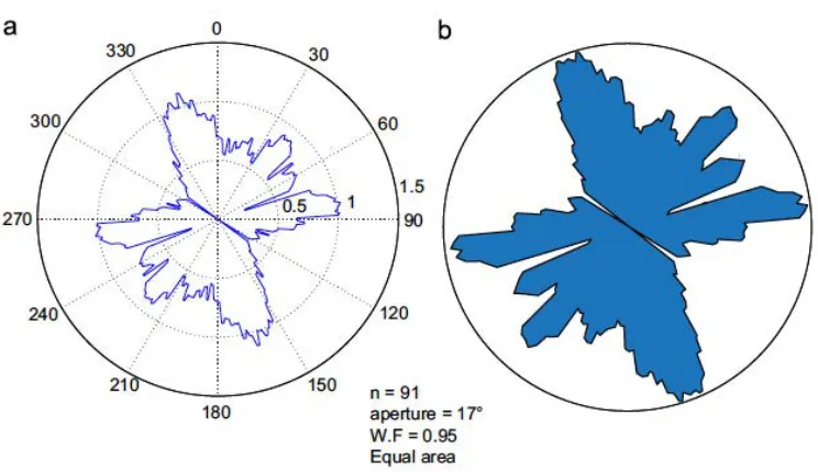
(27) Section A . M. A. Munro . whether the porphyroblasts have been subject to significant rotation during subsequent deformation events. Figs. 5, 6 and 7 depict long axis orientations of Syntarsis rhodesiensis (Dinosauria, theropoda) bones within a sedimentary sequence from Zimbabwe (Roberts et al, unpubl. data). These are considered bi-directional as opposed to the aforementioned uni-directional sets utilised for palaeocurrents because they are not associated with one specific azimuth (i.e. flow direction) and thus are represented as both. Additional applications of this function include the long axes orientations of igneous phenocrysts or granite bodies, (e.g. Blenkinsop & Treloar, 2001), dyke trends (Klausen, 2006), fault strikes (Wechsler et al., 2010), shear zone strikes (Blenkinsop et al., 1990) and the axial traces of folds. The latter are distinguished from fold hinges, which are uni-directional measurements.. 5.3 “Pitches/plunges” option (MATLAB® & Octave versions only). The “pitches/plunges” option is illustrated via the plotting of 2-Dimensional porphyroblast internal inclusion trail pitches from the classic Cooma Metamorphic Complex of S. E. Australia. The inclination of internal foliation pitches from the horizontal were measured directly from microscope thin sections using a mechanical stage. The inclusion trails were measured perpendicular to their strikes, in order to obtain their true pitches.. This was conducted for andalusite and cordierite. porphyroblasts (Fig. 9), both of which proved insightful in reconstructing the tectonometamorphic history of the complex.. The consistency of inclusion trail pitches. exhibited by the rose diagrams, in conjunction with other microstructural and. . 21 .
(28) Section A . M. A. Munro . mesoscale evidence, is highly suggestive that the inclusion trails are representative of their initial orientations.. Such pitch measurements have been made in several. publications on inclusion trails (e.g. Hayward, 1992; Johnson, 1992; Aerden, 1995), however the moving average rose diagrams presented here have a more informative appearance than the commonly utilised format of 10° binned data.. 6. CONCLUSIONS. Moving averages are an under-utilised form of analysis when dealing with circular, or vector, data in the Earth Sciences, perhaps because of the lack of moving average functionality in almost all available software used to produce rose diagrams. The dearth of moving average rose diagrams may be further enhanced by a lack of awareness of the benefits and potential use of moving averages when dealing with orientation data. To this end, MARD is presented in several formats such that it is readily available to the scientific community, and has been designed for ease-of-use. The examples of moving average rose diagrams above illustrates their broad applicability to numerous and diverse fields in Earth Sciences. They serve to reduce the background noise of the plots, and render significant trends readily apparent. When incorporating moving average rose diagrams in publications it is important to specify the number of elements within sample analysed, the aperture, whether linear scaling or equal area representations are used, and any weighting factor utilised in the on the figure or in the figure caption.. . Moreover, when plotting multiple rose. 22 .
(29) Section A . M. A. Munro . diagrams for comparison with one another in the same figure, we recommend utilising the same set of parameters in each.. . 23 .
(30) Section A . M. A. Munro . REFERENCES. Aerden, D.G.A.M., 1995. Porphyroblast non-rotation during crustal extension in the Variscan Lys-Caillaouas Massif, Pyrenees. Journal of Structural Geology, 17, 709-725. Aerden, D.G.A.M., 2003. Preferred orientation of planar microstructures determined via statistical best-fit of measured intersection-lines: the ‘FitPitch’ computer program. Journal of Structural Geology, 25, 923-934. Aerden, D.G.A.M., 2004.. Correlating deformation in Variscan NW-Iberia using. porphyroblasts; implications for the Ibero-Armorican Arc. Journal of Structural Geology, 26, 177-196. Aerden, D.G.A.M., & Sayab, M., 2008. From Adria- to Africa-driven orogenesis: Evidence from porphyroblasts in the Betic Cordillera, Spain.. Journal of. Structural Geology, 30, 1272–1287. Allmendinger, R.W., Cardozo, N., & Fisher, D.M., 2012.. Structural Geology. Algorithms, 1st Edn., Cambridge University Press, Cambridge, 289pp. Baas, J.H., 2000. EZ-ROSE: a computer program for equal-area circular histograms and statistical analysis of two-dimensional vectorial data.. Computers &. Geosciences, 26, 153-166. Behrensmeyer, A.K., 1982.. Time resolution in fluvial vertebrate assemblages.. Paleobiology, 8, 211-227. Behrensmeyer, A.K., 1987.. Vertebrate preservation in fluvial channels.. Palaeogeography, Palaeoclimatology, Palaeoecology, 63, 183-199. Berens, P., & Velasco, M.J., 2009. CircStat: A MATLAB Toolbox for Circular Statistics. Journal of Statistical Software, 31, issue 10.. . 24 .
(31) Section A . M. A. Munro . Blenkinsop, T. G., Dhilwayo, J., & Muranda, S.C. 1990. Intracratonic shearing on shear zones of the Mushandike granite, Zimbabwe. Proceedings of the Second Symposium of Science and Technology, Research Council of Zimbabwe, IIA, 396-421. Blenkinsop, T.G., & Kisters, A.F.M. 2005. Steep extrusion of late Archean granulites in the Northern Marginal Zone, Zimbabwe; evidence for secular change in orogenic style. Geological Society of London Special Publications, 243, 193204, doi:10.1144/GSL.SP.2005.243.01.14 Blenkinsop, T.G., & Treloar, P.J., 2001. Tabular intrusion and folding of the late Archaean Murehwa granite, Zimbabwe, during regional shortening. Journal of the Geological Society of London, 158, 653-664. Borradaile, G.J., 2003. Statistics of Earth Science data: their distribution in time, space and orientation, 1st Edn., Springer, 351pp. Davis, J.C., 2002. Statistics and Data Analysis in Geology, 3rd Edn., John Wiley & Sons, 656pp. Diniz da Costa, R., & Starkey, J., 2001. PhotoLin: a program to identify and analyze linear structures in aerial photographs, satellite images and maps. Computers & Geosciences, 27, 527-534. Eaton, J.W., Bateman, D., & Hauberg, S., 2008. GNU Octave Manual Version 3, Network Theory Limited, 568pp. Eberth, D.A., & Currie, P.J., 2010. Stratigraphy, sedimentology, and taphonomy of the. Albertosaurus. Bonebed. (upper. Horseshoe. Canyon. Formation;. Maastrichtian), southern Alberta, Canada. Canadian Journal of Earth Sciences, 47, 1119-1143. Fisher, N.I., 1993. Statistical Analysis of Circular Data, 1st Edn., Cambridge. . 25 .
(32) Section A . M. A. Munro . University Press, New York, NY, 277pp. Hayward, N., 1992. Microstructural analysis of the classical spiral garnet porphyroblasts of south-east Vermont: evidence for non-rotation. Journal of Metamorphic Geology, 10, 567-587. Holcombe, R.J., 1994. GEOrient - an integrated structural plotting package for MSWindows. Geological Society of Australia Abstracts, 36, 73-74. Johnson, S.E., 1992. Sequential porphyroblast growth during progressive deformation and low-P high-T LPHT) metamorphism, Cooma Complex, Australia: the use of micro- structural analysis to better understand deformation and metamorphic histories. Tectonophysics, 214, 311-339. Jones, T.A., 2006. MATLAB functions to analyze directional (azimuthal) data—I: Single-sample inference. Computers & Geosciences, 32, 166-175. Jordan, G., 2007. Adaptive smoothing of valleys in DEMs using TIN interpolation from ridgeline elevations: An application to morphotectonic aspect analysis. Computers & Geosciences, 33, 573-585. Klausen, M.B., 2006. Geometry and mode of emplacement of dike swarms around the Birnudalstindur igneous centre, SE Iceland. Journal of Volcanology and Geothermal Research, 151, 340-356. Kutty, T.S., & Ghosh, P., 1992. Rose.C: a program in `C' for producing high-quality rose diagrams. Computers & Geosciences, 18, 1195-1211. Nemec, W., 1988. The shape of the rose. Sedimentary Geology, 59, 149-152. Pewsey, A., 2004. The Large-Sample Joint Distribution of Key Circular Statistics. Metrika, 60, 25-32. Roberts, E.M., & Hendrix, M.S., 2000. Taphonomy of a Petrified Forest in the Two Medicine Formation (Campanian), Northwest Montana: Implications for. . 26 .
(33) Section A . M. A. Munro . Palinspastic Restoration of the Boulder Batholith and Elkhorn Mountain Volcanics. Palaios, 15, 476–482. Roberts, E.M., O’Connor, P.M., Stevens, N.J., Gottfried, M.D., Jinnah, Z.A., Ngasala, S., Choh, A.M., & Armstrong, R.A., 2010. Sedimentology and depositional environments of the Red Sandstone Group, Rukwa Rift Basin, southwestern Tanzania: New insight into Cretaceous and Paleogene terrestrial ecosystems and tectonics in sub-equatorial Africa. Journal of African Earth Sciences, 57, 179212. Tucker, R.T., 2011. Taphonomy of Sheridan College Quarry 1, Buffalo, Wyoming: Implications for reconstructing historic dinosaur localities including Utterback’s 1902–1910 Morrison dinosaur expeditions. Geobios, 44, 527–541. Voorhies, M.R., 1969. Taphonomy and population dynamics of an early Pliocene Vertebrate Fauna, Knox County, Nebraska. Contributions to Geology Special Paper No. 1, University of Wyoming, 69p. Wechsler, N., Ben-Zion, Y., & Christofferson, S., 2010. Evolving geometrical heterogeneities of fault trace data. Geophysical Journal International, 182, 551– 567. Wells, N.A., 1999. ASTRA.BAS: a program in QuickBasic 4.5 for exploring rose diagrams, circular histograms and some alternatives. Computers & Geosciences, 25, 641-654. Wells, N.A., 2000. Are there better alternatives to standard rose diagrams? Journal of Sedimentary Research, 70, 37-46.. . 27 .
(34) Section B . . M. A. Munro . - SECTION B -. PORPHYROBLAST MICROSTRUCTURES: A REVIEW OF STRATEGIES FOR THEIR OBSERVATION AND MEASUREMENT. . 28 .
(35) Section B . . M. A. Munro . PORPHYROBLAST MICROSTRUCTURES: A REVIEW OF STRATEGIES FOR THEIR OBSERVATION AND MEASUREMENT. Abstract ....................................................................................................................... 31 1. Introduction ............................................................................................................ 32 2. Techniques: outline ................................................................................................ 34 2.1 ‘P-N’ thin-sectioning ...................................................................................................... 34 2.2 Inclusion trail pitch measurements ................................................................................. 34 2.3 Measuring inclusion trail strikes .................................................................................... 35 2.4 The radial asymmetry method ........................................................................................ 36 2.5 Parallel serial thin sectioning ......................................................................................... 38 2.6 The “FitPitch” method ................................................................................................... 39 2.7 Electron backscatter diffraction (EBSD) measurement of inclusion trails .................... 40 2.8 High-Resolution X-ray Computed Tomography (HRXCT) .......................................... 41. 3. Cross-referencing the techniques ......................................................................... 43 3.1 Inclusion trail strike measurement vs. radial asymmetry method .................................. 43 3.2 HRXCT vs. radial asymmetry method ........................................................................... 44. 4. Techniques: advantages and restrictions ............................................................. 45 4.1 P-N sectioning ................................................................................................................ 45 4.2 Measuring inclusion trail strikes .................................................................................... 46 4.3 Radial asymmetry method .............................................................................................. 48 4.4 FitPitch ........................................................................................................................... 50 4.5 HRXCT .......................................................................................................................... 51. . 29 .
(36) Section B . . M. A. Munro . 4.6 Summary of technique capabilities ................................................................................ 52. 5. Conclusions ............................................................................................................. 53 References ................................................................................................................... 54. . 30 .
(37) Section B . . M. A. Munro . ABSTRACT. Porphyroblastic phases preserve a wealth of information pertaining to the P-T conditions experienced by the hosting metamorphic rocks. However, accurately interpreting the timing of the growth of porphyroblasts relative to one another and to matrix structures is not simple. Porphyroblast inclusion trail geometries range from straight, straight with inflected margins, to sigmoidal and spiral. Accordingly, this has required the development of a number of strategies for the examination, and qualitative and quantitative documentation of inclusion trails, each targeting different aspects of these geometries. This includes ‘P-N’ sectioning, pitch measurement, strike measurement, radial serial sectioning, parallel serial sectioning, best-fit plane assignment (‘FitPitch’) and High-Resolution X-ray Computed Tomography (HRXCT). Each technique has its own associated merits and restrictions, and is most effective when applied to different scenarios. Cross-referencing the findings of HRXCT, radial asymmetry, inclusion trail strike measurement and FitPitch with one another conveys that their results are in excellent agreement. Investigators must be mindful in the selection of their techniques as mounting evidence suggests that they risk potentially omitting key observations if utilizing a restricted number of perspectives based upon the orientations of matrix structures. A comprehensive documentation of the tectonometamorphic history preserved within porphyroblastic rocks may require the implementation of multiple techniques, even within a single sample.. Keywords:. Porphyroblasts, microstructure, inclusion trails, measurement, P-T-t-. deformation path. . 31 .
(38) Section B . . M. A. Munro . 1. INTRODUCTION. Porphyroblastic phases preserve a wealth of information pertaining to the tectono-metamorphic evolution that the hosting metamorphic rocks have experienced. This includes Pressure-Temperature constraints during their nucleation and the overgrowth and preservation of potentially multiple generations of foliation. However, accurately interpreting the timing of the growth of porphyroblasts relative to one another and to matrix structures is not simple (e.g. Vernon et al, 1993; Johnson & Vernon, 1995a). Timing of porphyroblast growth is crucial in reconstructing P-T-td trajectories for a region, and mis-interpretation may have profound implications for either the deformation component or the inferred metamorphic reactions (Johnson & Vernon, 1995b). The revelation that some internal foliations within porphyroblasts may pre-date those manifested in the matrix prompted a surge in microstructural investigation to substantiate whether these orientations may be utilized as reliable indicators of relict deformation events, despite ongoing controversy concerning the potential for porphyroblasts to rotate with respect to fixed geographical coordinates and other external reference frames (Bell et al, 1992; Passchier et al, 1992; Williams & Jiang, 1999; Kraus & Williams, 2001). Porphyroblast inclusion trail geometries vary, being entirely straight, straight with inflected margins, sigmoidal or spiral.. Accordingly, this has required the. development of a broad range of strategies for the examination, and qualitative and quantitative measurement of porphyroblasts, each targeting different aspects of their internal geometries. These include P-N sectioning (e.g. Bell & Rubenach, 1983), pitch measurement from vertical thin sections (Hayward, 1992; Johnson, 1992; Aerden, 1995), strike measurement from horizontal thin sections (e.g. Aerden 2004;. . 32 .
(39) Section B . . M. A. Munro . Aerden & Sayab, 2008), radial serial sectioning (Hayward, 1990; Bell et al, 1995), parallel serial sectioning (Johnson, 1993; Johnson & Moore, 1993; 1996), best-fit plane assignment (Aerden, 2003) and High-Resolution X-ray Computed Tomography, or HRXCT (Carlson et al, 2003; Ketcham & Carlson, 2001; Ikeda et al, 2002; Huddlestone-Holmes & Ketcham, 2005; 2010; Whitney et al, 2008). Whilst possessing the potential to transform understanding of the 3D internal geometries preserved in individual porphyroblasts, HRXCT and Synchrotron-based Microtomography are expensive, partly owing to the long analyses required to produce sufficient resolutions. Moreover, suitability of these techniques is dependent upon a range of factors including the sample size desired for analysis and phasedependent contrasts in linear attenuation coefficients between the host and its inclusions. Thus, they remain relatively unviable for routine application to adequate quantities of samples necessary for extracting valid structural and tectonic interpretations. Microscopy, by contrast, persists as the most readily accessible and relatively inexpensive means for the study and correlation of microstructures between multiple samples. However, an increasing number of studies have raised concerns that the microscopy strategies most commonly applied to the examination of porphyroblasts, such as ‘P-N’ sectioning, may yield incomplete information with significant observations undetected (e.g. Cihan, 2004). A number of new techniques have been devised and others refined since Johnson’s (1999) review of porphyroblast microstructure applications. Some of these techniques are designed to measure the same quantities and can therefore be compared to assess their accuracy. Currently, no contributions exist to summarize this and therefore this one is necessary. It provides an overview of each strategy, its. . 33 .
(40) Section B . . M. A. Munro . requirements for use, examines its findings when applied to the same rocks and evaluates its relative merits and limitations.. 2. TECHNIQUES: OUTLINE. The features of inclusion trail geometry specifically targeted by each of the thin-sectioning strategies are summarized in Fig. 1.. 2.1 ‘P-N’ thin-sectioning. This is the strategy most commonly applied to the analysis of porphyroblastic rocks. Typically 2, or perhaps 3, thin sections are produced; the orientations of which are dependent upon that of the dominant foliations present within the bulk matrix of the rock (e.g. Bell & Rubenach, 1983; Johnson et al, 2006). ‘P’ refers to those cut perpendicular to the foliation but parallel to the lineation and ‘N’ those perpendicular to the foliation but normal to the lineation (Fig. 2). Variations of this approach are straightforward and rapid to apply, do not require large sample volumes and are inexpensive relative to sophisticated imaging techniques.. 2.2 Inclusion trail pitch measurements. This method involves determining the pitch, or inclination, of intersection lineation that internal foliations make with an oriented vertical thin section plane.. . 34 .
(41) Section B . . M. A. Munro . Pitches are measured via a mechanical stage and represent values relative to a predefined artificial reference horizon (generally horizontal).. The objective of this. method is to quantify 1) the degree of consistency between individual porphyroblasts either within or between samples, and 2) whether the internal foliations are subhorizontal, sub-vertical or oblique. The main requirement is that the main body of the inclusion trail be straight to weakly sigmoidal. However, the method can also include measurements of straight or weakly curved truncations that are part of spiral-shaped inclusion trails (e.g. Aerden, 2003). Such datasets have been presented as an integral part of many studies which have engaged whether populations of porphyroblasts have rotated during later deformations, compromising their initial orientations (Hayward, 1992; Johnson, 1992; Aerden, 1995; Johnson et al, 2006).. Measurements are. conventionally represented in binned rose diagram format (e.g. Hayward, 1992; Johnson, 1992) however they may also be expressed effectively as moving average roses (e.g. Aerden, 2004; Aerden & Sayab, 2008; Munro & Blenkinsop, 2012). The most important consideration in either case is that roses should always be presented as equal area plots to eliminate the often-pronounced bias that frequently arises from linearly scaled rose diagrams (Nemec, 1988).. 2.3 Measuring inclusion trail strikes. Foliation strikes in horizontal thin sections (Fig. 1.) are determined via the same procedure as for pitches; the measurement of intersection lineations with the thin section plane. Here, individual measurements are determined relative to True North, which serves as a reference horizon. Whilst the straight sections of any inclusion trail may be measured, this technique primarily targets porphyroblasts. . 35 .
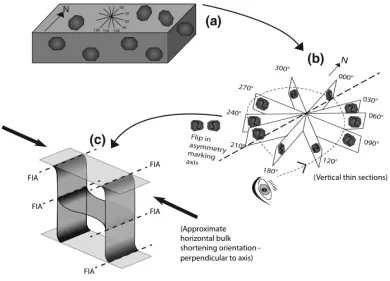
(42) Section B . . M. A. Munro . preserving steeply inclined to sub-vertical foliations; i.e. those that may furnish a horizontal bulk shortening orientation in an analogous manner to matrix foliations. Flat-lying internal foliations that anastamose on the other hand may produce an array of orientations in plan view that are relatively uninformative.. Studies have. demonstrated that the relative timing of successive overprinting, obliquely-striking, steep foliations may also be resolved within individual porphyroblasts in which one composes the core and the succeeding forms a rim (Aerden, 2004; Aerden & Sayab, 2008).. 2.4 The radial asymmetry method. The radial asymmetry approach to porphyroblast examination (Fig. 3) was first proposed by Hayward (1990) and subsequently elaborated upon by Bell et al. (1995). The technique utilizes the phenomenon that inclusion trails preserved within porphyroblasts exhibit an apparent switch in asymmetry from clockwise to anticlockwise (‘S’ to ‘Z’) or vice versa when viewed systematically around the compass (Fig. 4). The axis about which this flip occurs is expressed as the ‘Foliation Intersection/Inflection Axis’, or ‘FIA’.. Where both asymmetries are present. simultaneously, this signals close proximity to the axis. A FIA, as its name may suggest, has two potential interpretations: the first being that it represents a crenulation axis or the intersection between two successive foliations, implying two deformations, the second being that it represents the axis about which the porphyroblast became progressively rotated during its development (Bell et al, 1995), implying one deformation only. The measurement of this feature is independent of the interpretation of what it represents. As outlined in Fig. 3, the motivation for. . 36 .
(43) Section B . . M. A. Munro . ascertaining the axis is that, in the absence of significant post-growth rotation, it serves as a potential indicator of the approximate horizontal bulk shortening orientation contemporaneous with the porphyroblast’s growth. Initially, samples of minimum dimensions 10x10x10cm are orientated in the field with the flat panel of a compass and then extracted (Bell et al, 1995). Following subsequent re-orientation under laboratory conditions using a sandbox, six spatially orientated vertical thin sections are constructed at 30° increments around the compass (00°, 30°, 60°, 90°, 120°, 150°) to constrain the axis to within a 30° range by noting the switch in asymmetry between two of them. Each axis is then further constrained to within 10° via the examination of two additional vertical sections between those delineating the switch. Potentially, multiple switches may be observed at differing orientations within an individual rock if more than one distinct generation of porphyroblasts co-exists, or if a single generation has been differentially rotated throughout post-dating deformation. Additionally, individuals may exhibit different axes between their cores and rims. Where FIAs are expressed as a trend, as is the case in the majority of studies, they are regarded as bi-directional data. However, the radial asymmetry method also incorporates a means of ascertaining the plunge of the axis (Bell et al, 1995; Huddlestone-Holmes & Ketcham, 2005). This is carried out via essentially the same radial-sectioning procedure as that for the trend; this time from the asymmetries observed between systematically dipping thin sections that strike perpendicular to its pre-determined trend (Fig. 5.). Where both plunge and trend are determined, FIAs are notated as uni-directional data in the same manner as lineations. Where plunges have been determined, they have been reported to be very shallow (Bell et al, 1995; Bell et. . 37 .
(44) Section B . . M. A. Munro . al, 1998; Stallard et al, 2003; Timms, 2003; Gavin, 2004; Bell & Newman, 2006; Huddlestone-Holmes & Ketcham, 2005; 2010).. 2.5 Parallel serial thin sectioning. This technique, notably applied to examine spirals within garnet porphyroblasts (Johnson, 1993; Johnson & Moore, 1993; 1996) involves the cutting of multiple, approximately 1.25mm-spaced, parallel-striking thin sections through an individual porphyroblast in order to reconstruct a 3D visualization of its internal geometry. In order to provide maximum benefit, the intersection/inflection axis must first be determined via the radial asymmetry approach, or variation thereof, such that the optimal strike of parallel section arrays relative to this can be ascertained. The porphyroblasts are photomicrographed in each section and each slice is stacked sequentially to compile a pseudo-3D model. The information contained in each of the individual cross-sections may then be assigned mathematical functions and amalgamated to produce models that permit 3D manipulation (e.g. Fig. 6). The approach circumvents the problem of only being able to intersect each unique porphyroblast once, as in other approaches and having to make inferences and assumptions regarding its entire geometry from a single transection. However, in doing so, a portion of material between each thin section is inevitably lost during the production process. The applicability of parallel thin sectioning is also dependent upon the size of porphyroblasts present, however up to 6-10 sections have been successfully acquired for garnets of approximately 1cm in size (Johnson, 1993). A potential alternative suggested for smaller porphyroblasts involves serial grinding of the sample in conjunction with either photography of the hand sample (e.g.. . 38 .
(45) Section B . . M. A. Munro . Marschallinger, 1998) or SEM imaging (Williams, pers. comm), eliminating some material loss but destroying the sample.. If the block were polished after each. grinding increment, then it could be photographed under the microscope using reflective light to highlight the inclusion trails.. This strategy for porphyroblast. examination is therefore more suited to the detailed internal study of a few unique porphyroblasts as opposed to statistically valid numbers for tectono-metamorphic interpretations.. 2.6 The “FitPitch” method. Aerden (2003) developed the “FitPitch” computer program for the determination of potential best-fit planes for multiple planar microstructures in rocks. The program assigns these planes based upon the pitches of inclusion trails or other types of planar microstructures in differently orientated thin sections (horizontal, vertical or otherwise). While differently orientated vertical thin sections may be used alone to analyse porphyroblast inclusion trails (e.g. Johnson et al., 2006) best fit planes are best constrained when these are used in conjunction with strike measurements from horizontal thin sections. Generally, the greater the number of independent thin sections measured, the greater the constraints placed upon the bestfit planes. Studies to date have achieved good results using six differently orientated vertical thin sections (30° spacing) in addition to a horizontal one (e.g. Aerden, 2004; Aerden & Sayab, 2008). “Fitpitch” presents up to two or three planes, potentially distinguishing between independent generations of microstructures within an individual sample. The strike and dip of these best-fit planes (in highly-inclined to steeply dipping foliations) may be interpreted in a similar manner to matrix foliations.. . 39 .
(46) Section B . . M. A. Munro . 2.7 Electron backscatter diffraction (EBSD) measurement of inclusion trails Using garnet-rich schists from the Orlica-Śnieżnik Dome of the West Sudetes mountain range, Skrzypek et al. (2011) presented a method for the measurement of platy, or needle-shaped, inclusion mineralogy (e.g. ilmenite) within individual porphyroblasts using in-situ electron backscatter diffraction (EBSD).. Initially,. scanning electron microscope (SEM) images were used to confirm that apparent ilmenite needles in thin section represented the intersections of tabular crystals, supporting the inference that the shape-preferred orientation of ilmenite corresponds to a foliation plane. The lattice-preferred orientation of both matrix and inclusion trail ilmenite was measured via EBSD, with an initial comparison of matrix grains to the macroscopic foliation measurement serving as an internal validation of the technique. Comparison of the inclusion ilmenite to that in the matrix was then conducted to assess whether the inclusions correlated or were affiliated with a pre-dating structure. Processing of the EBSD results was carried out using PFch5 software (Mainprice, 2005) to determine a [100] and c [001] axis patterns for the illmenite, the latter representing the pole to the ilmenite platelet (Moseley, 1981). This data was then used to derive plane orientations with respect to geographical coordinates. The study demonstrated that matrix ilmentite a and c axes were well constrained and yielded a foliation plane orientation correlating with the associated mesoscale measurements. A minor discrepancy between the microscopically and mesoscopically determined orientations was inferred to represent deflection of the external matrix foliation around the competent porphyroblasts. Application of the same procedure to the garnet inclusion trails revealed their orientations to be in good agreement with those of earlier foliations that have been variably eliminated from the present matrix. These . 40 .
(47) Section B . . M. A. Munro . findings suggest that the technique provides an accurate means of determining foliation and lineation orientations from individual porphyroblasts as well as that of matrix grains. The authors noted that the technique is dependent upon the presence of a sufficient number of ilmenite inclusions within each individual porphyroblast, with approximately 20 grains appearing a reliable threshold. Moreover, it was suggested that other strongly anisotropic mineralogy such as mica might be suitable for defining inclusion trail geometries via this method, and that it is applicable to other porphyroblastic phases in addition to garnet.. 2.8 High-Resolution X-ray Computed Tomography (HRXCT). High-Resolution X-ray Computed Tomography (HRXCT) represents a relatively new technology that has seen continual refinements over the last couple of decades, facilitating the generation of progressively higher resolutions. The technique has found a broad range of applications within geology including igneous petrology (Ogasawara et al, 1998) sedimentology (Orsi & Anderson, 1995; Orsi et al, 1994) paleontology (Ketcham & Carlson, 2001) and the examination of meteorites (Arnold et al, 1982).. Pioneering investigations into metamorphic rocks focused primarily. upon the nucleation behaviour of porphyroblasts (Carlson & Denison, 1992; Denison & Carlson, 1997; Denison et al, 1997; Bauer et al, 1998; Carlson, 2006) and nondestructively establishing the size and spatial distribution of populations of garnet and staurolite within hand samples of schist (Ketcham & Carlson, 2001; Ketcham, 2005a,b; Ketcham et al, 2005). Research has subsequently progressed to provide the first truly three-dimensional representations of the internal geometries within individual garnet porphyroblasts (Huddlestone-Holmes & Ketcham, 2005; Ikeda et al, 2002; Bell & Bruce, 2006; Whitney et al, 2008). Following post-processing, the data. . 41 .
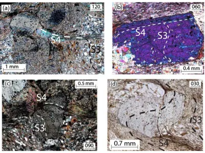
(48) Section B . . M. A. Munro . and resulting images may be manipulated to remove and isolate elements of the inclusion mineralogy to assist in visualization (Fig. 7). Tomography of this kind represents a significant advancement over conventional thin-sectioning as it eliminates the necessary degree of interpretation involved in reconciling what is observed between the different section orientations, each of which transect unique sets of porphyroblasts. Of the common porphyroblastic phases that characterize metamorphic rocks, garnet and staurolite are the most readily compatible for internal imaging due to exhibiting notably greater, and therefore sufficient contrasts in, linear attenuation coefficients relative to common inclusion constituents such as quartz, muscovite, biotite and ilmenite. Other porphyroblastic minerals such as andalusite, cordierite, kyanite and K-feldspar typically exhibit too similar a contrast to be routinely applicable (Fig. 8).. Huddlestone-Holmes & Ketcham (2005) outline a series of. guidelines for the consideration of prospective users of the technique for this purpose. Firstly, the attenuation of each material varies inverse proportionally to the intensity of X-ray energy applied to it (Fig. 8). Therefore, the contrast in attenuation between any two given minerals therefore also varies, generally showing a tendency to converge with increasing intensity.. Lower energies allow enhanced degrees of. sensitivity and may appear the intuitive choice for examination. However, this factor competes directly against X-ray penetration, which is less efficient at low energy (Huddlestone-Holmes & Ketcham, 2005). Thus, a compromise must be established to achieve successful results. Additionally, other effects such as ‘beam hardening’ and ‘ring artifacts’ may also impact upon the quality of the final images, requiring the implementation of a wedge calibration.. . 42 .
Figure
+7


Related documents
