https://doi.org/10.1051/0004-6361/201832860
c
ESO 2019
Astronomy
&
Astrophysics
Consistent dust and gas models for protoplanetary disks
IV. A panchromatic view of protoplanetary disks
?O. Dionatos
1, P. Woitke
2,3, M. Güdel
1, P. Degroote
4, A. Liebhart
1, F. Anthonioz
5, S. Antonellini
6,7,
C. Baldovin-Saavedra
1, A. Carmona
8, C. Dominik
9, J. Greaves
10, J. D. Ilee
11, I. Kamp
6, F. Ménard
5, M. Min
9,12,
C. Pinte
5,13,14, C. Rab
1,6, L. Rigon
2, W. F. Thi
15, and L. B. F. M. Waters
9,121 Department of Astrophysics, University of Vienna, Türkenschanzstrasse 17, 1180 Vienna, Austria
e-mail:odysseas.dionatos@univie.ac.at
2 SUPA School of Physics & Astronomy, University of St. Andrews, North Haugh, KY16 9SS St. Andrews, UK
3 Centre for Exoplanet Science, University of St. Andrews, St. Andrews, UK
4 Instituut voor Sterrenkunde, K.U. Leuven, Celestijnenlaan 200D, 3001 Leuven, Belgium
5 Univ. Grenoble Alpes, CNRS, IPAG, 38000 Grenoble, France
6 Kapteyn Astronomical Institute, University of Groningen, Postbus 800, 9700 AV Groningen, The Netherlands
7 Astrophysics Research Centre, School of Mathematics and Physics, Queen’s University Belfast, University Road,
Belfast BT7 1NN, UK
8 IRAP, Université de Toulouse, CNRS, UPS, Toulouse, France
9 Astronomical institute Anton Pannekoek, University of Amsterdam, Science Park 904, 1098 XH Amsterdam, The Netherlands
10 School of Physics and Astronomy, CardiffUniversity, 4 The Parade, CardiffCF24 3AA, UK
11 Institute of Astronomy, University of Cambridge, Madingley Road, Cambridge CB3 0HA, UK
12 SRON Netherlands Institute for Space Research, Sorbonnelaan 2, 3584 CA Utrecht, The Netherlands
13 UMI-FCA, CNRS/INSU France (UMI 3386), and Departamento de Astronomica, Universidad de Chile, Santiago, Chile
14 Monash Centre for Astrophysics (MoCA) and School of Physics and Astronomy, Monash University, Clayton, VIC 3800, Australia
15 Max-Planck-Institut für extraterrestrische Physik, Giessenbachstrasse 1, 85748 Garching, Germany
Received 20 February 2018/Accepted 22 February 2019
ABSTRACT
Context. Consistent modeling of protoplanetary disks requires the simultaneous solution of both continuum and line radiative transfer, heating and cooling balance between dust and gas and, of course, chemistry. Such models depend on panchromatic observations that can provide a complete description of the physical and chemical properties and energy balance of protoplanetary systems. Along these lines, we present a homogeneous, panchromatic collection of data on a sample of 85 T Tauri and Herbig Ae objects for which data cover a range from X-rays to centimeter wavelengths. Datasets consist of photometric measurements, spectra, along with results from the data analysis such as line fluxes from atomic and molecular transitions. Additional properties resulting from modeling of the sources such as disk mass and shape parameters, dust size, and polycyclic aromatic hydrocarbon (PAH) properties are also provided for completeness.
Aim. The purpose of this data collection is to provide a solid base that can enable consistent modeling of the properties of protoplan-etary disks. To this end, we performed an unbiased collection of publicly available data that were combined to homogeneous datasets adopting consistent criteria. Targets were selected based on both their properties and the availability of data.
Methods. Data from more than 50 different telescopes and facilities were retrieved and combined in homogeneous datasets directly from public data archives or after being extracted from more than 100 published articles. X-ray data for a subset of 56 sources repre-sent an exception as they were reduced from scratch and are prerepre-sented here for the first time.
Results. Compiled datasets, along with a subset of continuum and emission-line models are stored in a dedicated database and dis-tributed through a publicly accessible online system. All datasets contain metadata descriptors that allow us to track them back to their original resources. The graphical user interface of the online system allows the user to visually inspect individual objects but also compare between datasets and models. It also offers to the user the possibility to download any of the stored data and metadata for further processing.
Key words. stars: formation – circumstellar matter – stars: variables: T Tauri, Herbig Ae/Be – accretion, accretion disks –
astronomical databases: miscellaneous
1. Introduction
Knowledge is advanced with the systematic analysis and inter-pretation of data. This statement is especially valid in fields such
?
A copy of the X-ray data is only available at the CDS via
anony-mous ftp to cdsarc.u-strasbg.fr(130.79.128.5) or viahttp:
//cdsarc.u-strasbg.fr/viz-bin/qcat?J/A+A/625/A66
and systematically through meta-analysis to confirm existing and reveal new trends and global patterns.
The study of star and planet formation, in particular, is a field that requires extensive wavelength coverage for an appro-priate characterization of sources. Such coverage can only be obtained by combining data from different facilities and instru-ments, which, however come with very different qualities (e.g., angular and spectral resolution, sensitivity and spatial or spectral coverage). The importance of the study of protoplanetary disks is today even more pronounced when seen from the perspec-tive of planet formation and habitability. Protoplanetary disks are indeed the places where the complex process of planet formation takes place, described by presently two competing theories. The core accretion theory (Laughlin et al. 2004;Ida & Lin 2005), ini-tially developed to explain our Solar System architecture, posits collisional growth of submicron sized dust grains up to km-sized planetesimals on timescales of 105−107years, and further growth to Earth-sized planets by gravitational interactions. Once protoplanetary cores of ten Earth-masses have formed, the sur-rounding gas is gravitationally captured to form gas giant plan-ets. Alternatively, gravitational instabilities in disks may directly form planets on much shorter timescales (few thousand years), but require fairly high densities and short cooling timescales at large distances from the star (Boss 2009;Rice & Armitage 2009). The field is going through major developments following recent advances in instrumentation (e.g., ALMA, VLT/SPHERE Ansdell et al. 2016;Garufi et al. 2017, respectively) but also due to more complex and sophisticated numerical codes. This input challenges our understanding of disk evolution, so it becomes increasingly important to evaluate it and interpret the data in terms of physical disk properties such as disk mass and geome-try, dust size properties and chemical concentrations.
Observations of protoplanetary disks are challenging to interpret since physical densities in the disks span more than ten orders of magnitude, ranging from about 1015 particles per cm3in the midplane close to the star to typical molecular cloud
densities of 104 particles per cm3 in the distant upper disk
regions. At the same time, temperatures range from several 1000 K in the inner disk to only 10–20 K at distances of sev-eral 100 au. The central star provides high energy UV and X-ray photons which are scattered into the disk where they drive vari-ous non-equilibrium processes. The exact structure of the disks is not known, but it strongly affects the excitation of atoms and molecules and therefore their spectral appearance in form of emission lines. The morphology of the inner disk regions, for example, is expected to have a direct impact on the appearance of the outer disk. An inclined inner disk geometry or a puffed up morphology will cast shadows in the outer disk regions, while gaps may allow the direct illumination of the inner rim of the outer disk. Such complex disk topologies can be understood only through multiwavelength studies. Emission at short wavelengths (X-ray, UV, optical) links to the high-energy processes like mass accretion, stellar activity, and jet acceleration close to the star. Intermediate wavelengths (near to mid-IR) trace the nature and distribution of dust and gas in the inner disk, while observations at longer wavelengths provide information about the total mass and chemistry of the gas and dust in the most extended parts of the disk. A better understanding of these multiwavelength obser-vations requires consistent models that are capable of treating all important physical and chemical processes in detail, simultane-ously, in the entire disk.
In this paper we present a coherent, panchromatic observa-tional datasets for 85 protoplanetary disks and their host stars, and derive the physical parameters and properties for a subset
of 27 disks. The present collection was created as one of the two main pillars (the other being consistent thermochemical modeling) of the “DiscAnalysis” (DIANA)1 project, aiming to perform a homogeneous and consistent modeling of their gas and dust properties with the use of sophisticated codes such as ProDiMo (Woitke et al. 2009,2016; Kamp et al. 2010, 2017; Thi et al. 2011), MCFOST (Pinte et al. 2006,2009) and MCMax (Min et al. 2009). In the context of the DiscAnalysis project, data assemblies for each individual source along with model-ing results for both continuum and line emission are now pub-licly distributed through the “DiscAnalysis Object Database” (DIOD)2. The basic functionalities of the end-user interface of
DIOD is presented in AppendixA.
2. The data
The majority of the sample sources consists of Class II and III, T Tauri and Herbig Ae systems. Selected targets cover an age spread between∼1 and 10 million years and spectral types rang-ing from B9 to M3. Sources were selected based on availabil-ity and overlap of good qualavailabil-ity data across the electromagnetic spectrum. We avoided known multiple objects where disk prop-erties are known to be modified by the gravitational interaction of the companion and that at different wavelengths and angu-lar resolutions may appear as single objects. We also avoided highly variable objects and in most cases edge-on disk geometry, as in such configurations the stellar properties are not well con-strained and often remain unknown. In terms of sample demo-graphics, the sample consists of 13 Herbig Ae, 7 transition disks, 58 T Tauri systems along with 7 embedded (Class I) sources or systems in an edge-on configuration (TableC.1).
Most of the data presented here were retrieved from public archives but were also collected from more than 100 published articles. In a few cases, unpublished datasets were collected through private communications. An exception to the above is the X-ray data that were reduced for the purposes of this project and are presented in this paper for the first time. Datasets consist of photometric data points along with spectra, where available. Together, they provide a complete description of the spectral energy distribution (SED). Such data were assembled from more than 150 individual filters and spectral chunks observed with
∼50 different telescopes and facilities. Information on the gas content of disks is provided in the form of measured fluxes per transition for different atoms and molecules, and when available, as complete spectral line profiles.
A basic data quality check was performed using the follow-ing scheme: for data assembled from large surveys we propa-gated the original data quality flags; however, in cases that more datasets exist at the same or adjacent wavelengths, flags were modified to reflect inconsistencies and systematic (e.g., calibra-tion) errors. In all cases links to the relevant papers are main-tained so that the end-user can efficiently trace back the original data resources. An example showing different qualities of assem-bled data are given in the SED plots in Fig.1, while the complete collection of SEDs for all sources is provided as online material in Fig.C.1.
In the following sections we provide a detailed account of the major facilities or other resources used to assemble our data sample. An overview of the assembled photometric and spectro-scopic datasets per wavelength regime along with information
1 An EU FP7-SPACE 2011 funded project, http://www.
diana-project.com/.
ABAur
0.1 1.0 10.0 100.0 1000.0 10000.0
λ [μm] -16
-14 -12 -10 -8
log
ν
Fν
[e
rg/
cm
2/s
]
ANS TD1 JOHNSON STROMGREN VILNIUS TYCHO USNOB1 COUSINS GENEVA GALEX
SDSS
2MASS IRAS AKARI
WISE
SCUBA IRAC <UV> spec Spitzer IRS
LkCa15
0.1 1.0 10.0 100.0 1000.0 10000
λ [μm] -16
-14 -12 -10
log
ν
Fν
[e
rg/
cm
2/s
]
JOHNSON TYCHO USNOB1 COUSINS
SDSS
2MASS IRAS AKARI
WISE
SCUBA IRAC MIPS <UV> spec Spitzer IRS MWC480
0.1 1.0 10.0 100.0 1000.0
λ [μm] -12
-11 -10 -9 -8
log
ν
Fν
[e
rg/
cm
2/s
]
ANS JOHNSON TYCHO USNOB1 COUSINS GENEVA GALEX
SDSS
2MASS IRAS AKARI
WISE
SCUBA <UV> spec Spitzer IRS
ABAur MWC480 LkCa15
Fig. 1.Example of “raw” collected data represented as SED diagrams for three sources (top row). Data for AB Aur (left panel) delineate well the
stellar and disk emission and show little scatter. The same is true for MWC 480 (mid panel), the Akari data points however show some deviation when compared to theSpitzer/IRS spectra. For a weaker source like LkCa 15 (right panel), the scatter is significant due to certain, not well pointed observations, and therefore the SED is not well defined. SED plots for all sources are given as online data in Fig.C.1.Lower rowpresents the actual modeled data for the three sources, after being hand-selected for consistency.
on the number of line fluxes and high resolution imaging infor-mation for each individual source is provided in TableC.1.
2.1. X-rays
While X-rays do not provide direct information about the disk, they can represent an important part of the total stellar radiation field which is directly affects the physical and chemical struc-ture of the disk. We mined the XMM-Newton3 (Jansen et al. 2001) and Chandra4 (Weisskopf et al. 2000) mission-archives
for X-ray observations of our target-list and obtained data for 56 sources (Table 1). X-ray data was extracted by using the SAS software (version 12.0.1) for the XMM-Newton data and the CIAO software (version 4.6.1) for the Chandra data. The CALDB calibration data used for the spectral extraction of the
Chandradata were taken from version 4.6.2., while the
XMM-Newtoncalibration data is put on a rolling release and thus has no
version number. In order to get the source spectra, we selected a circular extraction region around the center of the emission, while the background area contained a large source-free area on the same CCD. The extraction tools (EVSELECT for XMM and SPECEXTRACT forChandra) delivered the source and back-ground spectra as well as the redistribution matrix and the ancil-lary response files.
The spectra were modeled by using the package XSPEC (Arnaud 1996), assuming a plasma model (VAPEC – an emis-sion spectrum for colliemis-sionally ionized diffuse plasma, based on the ATOMDB code [v.2.0.2]) combined with an absorption
col-3 http://xmm.esac.esa.int/xsa/
4 http://cxc.harvard.edu/cda/
umn model (WABS) based on the cross-sections fromMorrison & McCammon (1983). The element abundance values in the VAPECmodels were set to typical values for premain sequence stars, as chosen by the XEST project (see also Table2,Güdel et al. 2007), unless otherwise noted in Table2. Either a one com-ponent (1T), a two comcom-ponent (2T) or a three comcom-ponent (3T) emission model is fitted to the data. Highly absorbed sources or scarce data allow only for 1T fits. In some cases sources show such a high absorption that it is impossible to fix the higher tem-perature due to low constraints on the slope of the harder (mean-ing more energetic>1 keV) part of the spectrum. In both these cases the higher temperature was fixed to 10 keV. The fit delivers the absorption column density toward the sourceNH, the plasma
emission temperatureTXfor each component. Finally, the
unab-sorbed spectrum is calculated after setting the absorption column density parameter to zero, and the flux is derived by integrating over the energy range from 0.3 to 10 keV. Hardness is defined by HH−+SS, withH andS denoting the hard part (1–10 keV) and the soft part (0.3–1 keV) of the spectrum respectively. Thus the hardness factor delivers a value between 1 and−1, showing a hard spectrum in the case of∼1 and a soft spectrum in the case of∼−1. Results from the fitting process are given in Table3.
2.2. Ultraviolet
Ultraviolet data were collected from different resources. Spectra were obtained from the archives of the International Ultravio-let Explorer (IUE)5, the Far Ultraviolet Spectroscopic Explorer
Table 1.List of X-ray observations.
Source Instrument Obs-ID Exposure time (104s)
DO Tau XMM-Newton 0501500101 2.46
DN Tau XMM-Newton 0651120101 10.2
VZ Cha XMM-Newton 0300270201 10.9
TW Cha XMM-Newton 0152460301 2.61
IM Lup XMM-Newton 0303900301 2.49
V806 Tau XMM-Newton 0203540301 2.95
RECX15 XMM-Newton 0605950101 4.00
GM Aur XMM-Newton 0652330201 3.07
DM Tau XMM-Newton 0554770101 3.37
TW Hya XMM-Newton 0112880201 2.38
CY Tau Chandra 3364 1.77
UY Aur XMM-Newton 0401870501 3.19
UZ Tau E XMM-Newton 0203541901 3.13
IQ Tau XMM-Newton 0203541401 2.84
GG Tau XMM-Newton 0652350201 1.43
FS Tau XMM-Newton 0203541101 3.43
HL Tau XMM-Newton 0109060301 4.86
Haro 6-5B XMM-Newton 0203541101 3.43
VW Cha XMM-Newton 0002740501 2.78
RW Aur XMM-Newton 0401870301 3.02
WW Cha XMM-Newton 0203810101 2.30
V709 CrA XMM-Newton 0146390101 2.87
FK Ser XMM-Newton 0403410101 0.25
T Tau N XMM-Newton 0301500101 6.69
DoAr 24E Chandra 3761 9.11
V853 Oph Chandra 622 0.48
HD97048 XMM-Newton 0002740501 2.80
HD31648 Chandra 8939 0.98
HD169142 Chandra 6430 0.99
T Cha XMM-Newton 0550120601 0.52
HD142527 XMM-Newton 0673540501 1.08
RU Lup XMM-Newton 0303900301 2.49
RY Lup XMM-Newton 0652350501 0.49
HD100546 Chandra 3427 0.26
HD163296 Chandra 3733 1.92
AB Aur XMM-Newton 0101440801 12.3
HD135344 Chandra 9927 3.17
LkCa15 Chandra 10999 0.98
HD150193 Chandra 982 0.29
UX Tau A Chandra 11001 0.50
RNO90 XMM-Newton 0602731101 0.78
AS205 XMM-Newton 0602730101 0.53
Sz68 XMM-Newton 0652350401 0.69
DG Tau XMM-Newton 0203540201 2.49
TWA7 Chandra 11004 0.14
RY Tau XMM-Newton 0101440701 4.09
BP Tau XMM-Newton 0200370101 11.5
DR Tau XMM-Newton 0406570701 0.96
Haro1-16 XMM-Newton 0550120201 1.54
GO Tau XMM-Newton 0203542201 2.66
CI Tau XMM-Newton 0203541701 2.60
EX Lup XMM-Newton 0551640201 6.56
WX Cha XMM-Newton 0002740501 2.77
XX Cha XMM-Newton 0300270201 10.9
AA Tau XMM-Newton 0152680401 1.37
HD142666 XMM-Newton 0673540801 0.85
(FUSE)6and theHubbleSpace Telescope (HST)7.Hubbledata
originate from three instruments, namely the Space Telescope Imaging Spectrograph (STIS), the Cosmic Origins Spectrograph (COS) and the Advanced Camera for Surveys (ACS).
6 https://archive.stsci.edu/fuse/
7 https://archive.stsci.edu/hst/
HD163296
900 1000 1200 1400 1600 2000 2500 3000 3500
λ [A] 10-15
10-14 10-13 10-12 10-11
Fλ
[e
rg/
cm
2/s
/A
]
IUE_LWP08767RL , 2399.7s
IUE_LWP08771RL , 2399.7s IUE_LWP08778RL , 2399.7s
IUE_LWP08779RL , 2399.7s IUE_LWP08782RL , 2399.7s IUE_LWP08783RL , 2399.7s IUE_LWP08793RL , 2399.7s
IUE_LWP08795RL , 2399.7s
IUE_LWP08796RL , 2399.7s IUE_LWP08803RL , 2399.7s
IUE_LWP08804RL , 2399.7s IUE_LWP08806RL , 2099.5s IUE_LWP08807RL , 2099.5s IUE_LWP30190RL , 3598.8s
IUE_SWP25391LL , 1199.6s
IUE_SWP28776LL , 1199.6s IUE_SWP28777LL , 1079.6s
IUE_SWP28778LL , 1079.6s IUE_SWP28781LL , 1079.6s + 12 further IUE files
FUSE_E5100801000 , 791.0s
FUSE_P2190601000 , 7076.0s FUSE_Q2190101000 , 6946.0s
STIS_o4xn05040_x1d , 1600.0s STIS_o57z03010_x1d , 2230.0s STIS_o66q01010_x1d , 1144.0s STIS_o66q01020_x1d , 432.0s
STIS_o66q01030_x1d , 2760.0s
STIS_o66q02010_x1d , 2282.0s STIS_o66q02020_x1d , 2904.0s
STIS_o66q03010_x1d , 7706.8s
[image:4.595.58.273.110.678.2]IUE_HD163296_a.txt UV_HD163296.dat
Fig. 2.Ultraviolet spectrum of HD163296, consisting of a series of
[image:4.595.311.549.369.634.2]indi-vidual observations from HST, FUSE and IUE. Black line represents the co-added spectrum of all observations as described in AppendixB.
Table 2. Standard XEST abundances and deviations for particular
sources used in theVAPECmodels.
Element XEST abundance Source Element Modified abundance
He 1 TW Cha Mg 0.917
C 0.450 Fe 0.222
N 0.788 GM Aur O 0.103
O 0.426 UZ Tau E O 2.704
Ne 0.832 HL Tau Mg 1.500
Mg 0.263 S 1.500
Al 0.500 Ca 1.500
Si 0.309 Fe 0.740
S 0.417 RW Aur FeI 0.058
Ar 0.550 FeII 0.456
Ca 0.195 V709 CrA O 0.308
Fe 0.195 FeI 0.079
Ni 0.195 FeII 0.207
FK Ser O 0.098
T Tau N O 0.193
FeI 0.052
FeII 0.074
HD31648 Ne 0.056
RU Lup FeI 0.140
FeII 0.614
TWA7 Fe 0.121
BP Tau Fe 0.047
WX Cha Fe 0.098
AA Tau Fe 0.491
Table 3.Results from the X-ray reduction.
Source NH Flux Fluxsoft Fluxhard Hardness Fabs Fabs−soft Fabs−hard Hardness T1 T2
(1022cm−2) (10−13erg cm−2s−1) (10−13erg cm−2s−1) (106K) (107K)
HD169142 0.0 0.538 0.516 0.022 −0.920 0.538 0.516 0.022 −0.920 2.71 0.0
RY Lup 0.724 30.9 27.4 3.480 −0.774 2.230 0.577 1.660 0.483 2.46 1.22
TW Hya 0.063 62.3 53.6 8.650 −0.722 39.3 31.3 7.960 −0.595 2.27 0.795
AB Aur 0.153 2.530 2.130 0.4 −0.684 1.060 0.730 0.327 −0.380 2.02 0.767
FK Ser 0.287 33.9 27.2 6.710 −0.605 9.120 4.110 5.010 0.099 2.58 1.49
HD31648 0.397 2.210 1.750 0.457 −0.586 0.543 0.258 0.285 0.050 6.56 0.0
FS Tau 1.702 46.6 36.3 10.3 −0.557 5.410 0.028 5.380 0.990 2.7 3.45
HD142527 0.181 1.430 1.1 0.325 −0.545 0.663 0.374 0.289 −0.128 3.35 11.6
GM Aur 0.285 7.820 5.960 1.850 −0.526 2.430 0.942 1.490 0.225 2.75 2.34
EX Lup 0.364 1.830 1.340 0.489 −0.466 0.533 0.089 0.444 0.667 1.92 17.4
HD135344 0.0 1.360 0.987 0.371 −0.453 1.360 0.987 0.371 −0.453 7.05 0.0
VW Cha 0.453 22.2 14.7 7.5 −0.324 6.610 1.440 5.160 0.563 3.93 2.12
WW Cha 0.709 15.8 10.4 5.380 −0.319 3.610 0.405 3.2 0.775 4.46 2.84
AA Tau 2.174 12.8 8.360 4.450 −0.306 1.0 0.007 0.994 0.986 10.0 3.17
TW Cha 0.173 3.490 2.240 1.260 −0.280 1.880 0.782 1.1 0.167 3.95 2.51
Sz68 0.362 11.6 7.410 4.210 −0.276 4.040 1.120 2.920 0.444 4.32 1.55
HD163296 0.001 2.720 1.730 0.996 −0.268 2.710 1.710 0.995 −0.265 6.3 12.6
LkCa15 0.233 7.060 4.340 2.720 −0.228 3.520 1.170 2.350 0.337 4.24 6.77
DN Tau 0.072 6.170 3.710 2.450 −0.204 4.510 2.220 2.280 0.013 5.35 2.28
CY Tau 0.0 0.274 0.161 0.113 −0.174 0.274 0.161 0.113 −0.174 11.0 0.0
UX TauA 0.104 7.360 4.250 3.110 −0.156 5.060 2.270 2.790 0.102 8.09 1.67
DM Tau 0.196 10.5 6.080 4.440 −0.156 5.560 1.780 3.780 0.359 3.56 1.91
WX Cha 0.411 9.260 5.140 4.120 −0.111 3.840 0.552 3.290 0.712 3.69 3.44
UZ TauE 0.264 1.790 0.980 0.812 −0.094 0.897 0.244 0.652 0.455 10.3 2.08
Haro1-16 0.276 5.720 3.070 2.650 −0.074 2.890 0.737 2.150 0.489 7.34 2.91
GG Tau 0.084 1.730 0.914 0.820 −0.054 1.3 0.532 0.773 0.184 5.26 3.84
T Cha 0.987 21.6 11.3 10.3 −0.044 5.560 0.231 5.330 0.917 9.71 2.32
DO Tau 1.127 1.370 0.703 0.663 −0.029 0.274 0.010 0.264 0.926 12.5 0.0
UY Aur 0.071 1.680 0.854 0.823 −0.019 1.320 0.544 0.779 0.178 9.2 3.08
HD100546 0.107 1.2 0.605 0.599 −0.005 0.845 0.310 0.535 0.266 13.0 0.0
BP Tau 0.086 7.940 3.930 4.010 0.010 5.9 2.140 3.760 0.275 5.6 2.92
GO Tau 0.344 0.781 0.379 0.403 0.030 0.389 0.065 0.324 0.666 6.29 3.49
IM Lup 0.093 10.3 4.950 5.380 0.042 7.750 2.750 5.0 0.291 9.54 2.49
XX Cha 0.272 2.250 1.080 1.170 0.043 1.230 0.260 0.968 0.576 9.05 2.78
TWA7 0.0 36.5 17.1 19.5 0.066 36.5 17.1 19.5 0.066 7.7 5.4
V806 Tau 1.227 1.510 0.703 0.808 0.069 0.385 0.007 0.378 0.962 12.5 11.8
T TauN 0.265 34.0 15.1 18.9 0.111 19.2 3.210 16.0 0.665 5.6 3.09
RNO90 0.631 22.7 9.790 12.9 0.137 9.6 0.574 9.030 0.880 8.89 2.82
RU Lup 0.144 8.360 3.6 4.760 0.139 5.890 1.520 4.370 0.485 7.33 5.01
V709 CrA 0.227 91.3 38.2 53.1 0.164 56.5 9.960 46.5 0.647 5.86 3.7
DR Tau 0.214 1.650 0.674 0.972 0.181 1.060 0.205 0.857 0.614 9.15 3.51
RECX15 0.073 0.492 0.197 0.295 0.2 0.408 0.123 0.284 0.394 7.39 6.58
V853 Oph 0.043 9.850 3.830 6.020 0.222 8.620 2.760 5.850 0.359 33.0 1.14
IQ Tau 0.533 4.530 1.720 2.810 0.242 2.240 0.139 2.1 0.876 11.5 3.14
HD150193 0.0 8.2 2.950 5.250 0.281 8.2 2.950 5.250 0.281 6.48 4.97
RY Tau 0.567 19.6 6.910 12.7 0.295 10.4 0.456 9.940 0.912 5.89 4.13
HL Tau 2.547 14.0 4.840 9.140 0.308 4.110 0.001 4.110 1.0 23.8 0.398
CI Tau 0.339 0.774 0.237 0.537 0.386 0.488 0.035 0.453 0.856 79.6 1.97
AS205 1.739 2.430 0.722 1.7 0.405 0.979 0.001 0.978 0.998 33.1 0.0
RW Aur 0.209 57.9 17.0 40.9 0.413 42.4 4.810 37.6 0.773 7.18 7.26
HD97048 0.162 0.201 0.054 0.148 0.467 0.156 0.018 0.138 0.764 40.7 0.0
VZ Cha 0.211 5.710 1.520 4.190 0.468 4.3 0.444 3.860 0.794 10.4 6.01
DoAr 24E 1.071 3.730 0.864 2.870 0.538 2.130 0.010 2.120 0.991 53.6 0.0
Haro 6-5B 1.814 1.080 0.236 0.848 0.564 0.565 0.0 0.565 0.999 60.3 0.0
DG Tau 0.043 1.520 0.205 1.310 0.730 1.460 0.153 1.310 0.791 4.46 2.4
– IUE’s short and long wavelength spectroscopic cameras pro-vided low resolution (R ≈400) spectra covering the 1150– 1980 Å and 1850–3350 Å windows, respectively. Often, a large number of data files exists per source in the archive8, however we have typically used the first∼20 with the longest integration times for each source. IUE averaged spectra as treated inValenti et al.(2000,2003) were collected for com-parisons but not used, as we combine IUE data along with spectra from other instruments.
– The Far Ultraviolet Spectroscopic Explorer (FUSE) covers the important 900–1190 Å band in high resolution (R ≈
20 000). The FUSE data may be affected by a number of emission lines due to the residual Earth atmosphere, also known as “airglow”. At first, FUSE data on faint disk sources may appear quite noisy, however combining and processing as described in AppendixBcan lead to high quality data in the very important region around 1000 Å.
– The HST Cosmic Origins Spectrograph (COS) and Space Telescope Imaging Spectrograph (STIS) cover wavelengths 1150–3600 Å and for our purposes the range 1150–3200 Å in very different resolutions up to R & 10 000. High res-olution data come in chunks that rarely cover large wave-length ranges, so they need to be combined. Combined HST datasets including lower resolution ACS data, are provided inYang et al.(2012)9.
The original datasets are therefore inhomogeneous, as they orig-inate from different instruments with different resolutions, inte-gration times and sensitivities. Moreover, some sources were tar-geted multiple times with a number of different instruments (see also Table 4). Intrinsic variation in the UV spectra as a result of changing accretion rates is expected, it is however beyond the scope of this study. As a first step, exceedingly noisy spec-tra were discarded after visual inspection. We note that IUE data shortward of the Lyα(λ≈1215 Å) show abnormally high fluxes when compared to HST/COS spectra and were consequently not used. IUE data longward of about 3100 Å can become exceed-ingly noisy and were also disregarded. We also note that while UV data of high quality exist for sources with spectral type rang-ing fromAtoM, data for theKandM-type stars either are sparse or do not exist.
An example of a co-added UV spectrum is presented in Fig.2 for HD 163296, while more plots for all other sources are pro-vided as online material in Fig.C.2.
For the cases that UV spectra were not available, we have collected photometric data points from a number of space facili-ties, namely:
– The Ultraviolet Sky Survey Telescope (UVSST) onboard the TD1 satellite (Humphries et al. 1976), provides photometry down to 10th mag in four UV 4 bands at 1565 Å, 1965 Å, 2365 Å and 2740 Å.
– The ultraviolet photometer of the Astronomical Netherlands Satellite (ANS) having five bands at 1500 Å, 1800 Å, 2500 Å and 3300 Å (Wesselius et al. 1982).
– The Galaxy Evolution Explorer (GALEX) mission provided wide band photometry in two windows; the FUV channel between 1350 and 1750 Å and the NUV channel between 1750 and 2800 Å (Morrissey et al. 2007).
8 http://sdc.cab.inta-csic.es/cgi-ines/IUEdbsMY
9 http://archive.stsci.edu/prepds/ttauriatlas/table.
[image:6.595.318.539.98.772.2]html
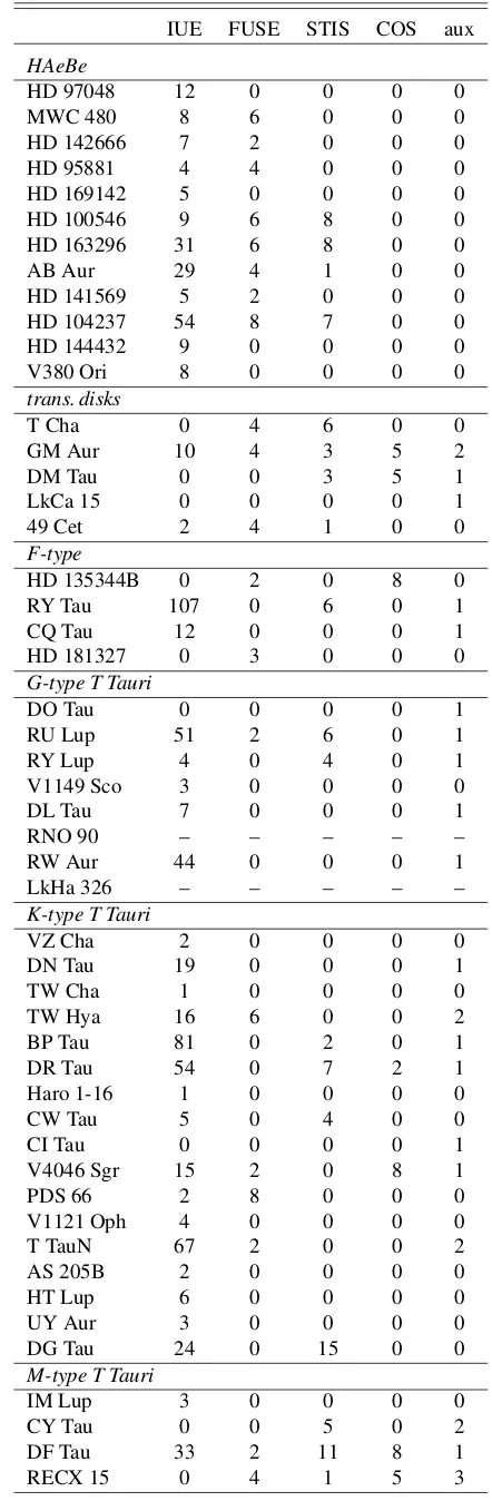
Table 4.Number of archival UV data files collected.
IUE FUSE STIS COS aux
HAeBe
HD 97048 12 0 0 0 0
MWC 480 8 6 0 0 0
HD 142666 7 2 0 0 0
HD 95881 4 4 0 0 0
HD 169142 5 0 0 0 0
HD 100546 9 6 8 0 0
HD 163296 31 6 8 0 0
AB Aur 29 4 1 0 0
HD 141569 5 2 0 0 0
HD 104237 54 8 7 0 0
HD 144432 9 0 0 0 0
V380 Ori 8 0 0 0 0
trans. disks
T Cha 0 4 6 0 0
GM Aur 10 4 3 5 2
DM Tau 0 0 3 5 1
LkCa 15 0 0 0 0 1
49 Cet 2 4 1 0 0
F-type
HD 135344B 0 2 0 8 0
RY Tau 107 0 6 0 1
CQ Tau 12 0 0 0 1
HD 181327 0 3 0 0 0
G-type T Tauri
DO Tau 0 0 0 0 1
RU Lup 51 2 6 0 1
RY Lup 4 0 4 0 1
V1149 Sco 3 0 0 0 0
DL Tau 7 0 0 0 1
RNO 90 – – – – –
RW Aur 44 0 0 0 1
LkHa 326 – – – – –
K-type T Tauri
VZ Cha 2 0 0 0 0
DN Tau 19 0 0 0 1
TW Cha 1 0 0 0 0
TW Hya 16 6 0 0 2
BP Tau 81 0 2 0 1
DR Tau 54 0 7 2 1
Haro 1-16 1 0 0 0 0
CW Tau 5 0 4 0 0
CI Tau 0 0 0 0 1
V4046 Sgr 15 2 0 8 1
PDS 66 2 8 0 0 0
V1121 Oph 4 0 0 0 0
T TauN 67 2 0 0 2
AS 205B 2 0 0 0 0
HT Lup 6 0 0 0 0
UY Aur 3 0 0 0 0
DG Tau 24 0 15 0 0
M-type T Tauri
IM Lup 3 0 0 0 0
CY Tau 0 0 5 0 2
DF Tau 33 2 11 8 1
Table 4.continued.
IUE FUSE STIS COS aux
EX Lup 3 0 0 0 0
XX Cha 0 2 0 0 0
GQ Lup 2 0 0 0 0
Hen 3-600A 1 0 6 0 1
UZ Tau E 0 0 0 0 1
TWA 7 0 0 0 0 1
FS Tau 0 0 2 0 0
edge-on disks
AA Tau 7 0 1 4 1
2.3. Visual
Visual data are considered the photometric data in all major photometric systems that can traditionally be observed from ground based facilities. Visual data have been collected using customized query scripts that scan and automatically retrieve data from online data archives. Such resources include:
– The Amateur Sky Survey (TASS) of the Northern Sky, mea-sured Mark IV magnitudes which are then converted to Johnson-CousinsV- andI-magnitudes (Richmond 2007). – General Catalog of Photometric Data II (GCPD), was queried
for standard photometric systems (Mermilliod et al. 1997). – Sloan Digital Sky Survey Photometric Catalog, release
8 (Adelman-McCarthy 2011) and release 6 ( Adelman-McCarthy et al. 2008).
– DENIS J–K photometry (Kimeswenger et al. 2004). – USNO-B1 All Sky Catalog (Monet et al. 2003).
– VizieR Online Data Catalog: Homogeneous Means in the UBV System (Mermilliod 2006).
– The Geneva-Copenhagen survey of the solar neighbourhood. III. Improved distances, ages, and kinematics (Holmberg et al. 2009).
– Catalog of stars measured in the Geneva Observatory photo-metric system (Rufener 1988).
– VizieR Online Data Catalog: Catalog of Stellar Photometry in Johnson’s 11-color system (Ducati 2002).
– All-sky compiled catalog of 2.5 million stars, comprising data from Hipparcos, Tycho, PPM and CMC11 catalogs
(Kharchenko 2001).
– UBVRIJKLMNH photoelectric photometric catalog (Morel & Magnenat 1978).
– Uvby β photoelectric photometric catalog (Hauck & Mermilliod 1998).
– Uvby β photometry of 1017 stars earlier than G0 in the Centaurus-Crux-Musca-Chamaeleon direction (Corradi & Franco 1995).
– Tycho-2 bright source catalog (Høg et al. 2000).
– The HipparcosandTychocatalogs (ESA 1997).
– SDSSg,r,i,z filters calculated from Hipparcos and Tycho
data (Ofek 2008).
– Catalog of photoelectric photometry in the Vilnius system (Straizys et al. 1989).
– Hipparcoscatalog photometric filters (Perryman et al. 1997)
The offset positions for different sets of observations along with proper motion vectors were visually inspected and subsequently selected or deselected by hand. In order to maintain homogeneity in our datasets, fluxes and corresponding errors were converted from original units to Jy. Data from different catalogs were cross-correlated and checked against and flags were applied according
to their quality. If no flux errors were given in the original cata-logs, a nominal 10% error was assumed, which sometimes was increased to 30% for particularly unreliable passbands.
There are some noticeable trends among the collected visual datasets. The SDSS data, for example, are of high quality but the survey was designed to be deep, so that background sources are sometimes confused with our intended targets. Such cases are easily identifiable and corrected. Photometric data from DENIS/VLTI are often saturated for rather bright sources, and in such cases data are flagged as unreliable. Data from the USNO-B1 survey suffer from rather high uncertainties, esti-mated between 30 and 50%, and the photometric filters of the survey are not well defined (Monet et al. 2003).
2.4. Near-infrared
For the purposes of the present data collection, near-infrared lies between 0.8 (i.e., the JohnsonIband) and∼2.2µm (KS band). In addition to the references from the Visual wavelengths that also apply here in some cases (the DENIS/VLTI datasets, for example), near infrared data were additionally collected from the following resources:
– Two Micron All Sky Survey (2MASS) (Cutri et al. 2012, 2003).
– The Cosmic Background Explorer (COBE) Diffuse Infrared Background Experiment (DIRBE) Point Source Catalog (Smith et al. 2004).
– J,H, andKsfor sources in Chameleon were retrieved from Carpenter et al.(2002).
2.5. Mid- and far-infrared
Mid- and far-infrared refers here to photometric and spectro-scopic data data between 5 and 200µm, observed mainly with space facilities. Data collection in this wavelength range con-sists of already reduced and previously published data, and quite often different reductions of the same dataset exist. The wave-length range is of particular importance for the proper model-ing of the dust content in disks. Therefore special care has been taken in order to evaluate the different datasets and reductions, in order to provide high quality data of silicate features, especially the most intense one centered at∼10µm.
The mid- and far-infrared data were collected from the fol-lowing resources:
– The Faint Source Catalog (Moshir 1990) of the Infrared Astronomical Satellite (IRAS;Helou & Walker 1988)
– Spitzer spectra from “Dust Evolution in Protoplanetary
Disks Around Herbig Ae/Be Stars” (Juhász et al. 2010)
– Spitzer data from the Cores 2 Disks (c2d) Survey (Evans
et al. 2003;Wahhaj et al. 2010).
– Smoothed ISO spectra for a sample of Herbig Ae/Be systems (Meeus et al. 2001).
– Spectra from the “SpitzerInfrared Spectrograph Survey of T-Tauri Stars in Taurus” (Furlan et al. 2011).
– SpitzerIRAC data from “Galactic Legacy Infrared Midplane
Survey Extraordinaire (GLIMPSE)” (Spitzer Science 2009).
– SpitzerIRAC and MIPS, data from “The Disk Population of
the Taurus Star-Forming Region” (Luhman et al. 2010).
– SpitzerIRAC data from “TaurusSpitzerSurvey: New
Candi-date Taurus Members Selected Using Sensitive Mid-Infrared Photometry” (Rebull et al. 2010).
– Spitzer spectrophotometric data from “The Formation and
– Data from the “The Cornell Atlas of Spitzer/IRS Sources (CASSIS10)” (Lebouteiller et al. 2011).
– Data from theSpitzerMap of the Taurus Molecular Clouds (Rebull et al. 2011).
– AKARI/IRC mid-infrared all-sky survey (Murakami et al. 2007;Ishihara et al. 2010).
– Spitzer/IRS data from the “The Different Evolution of Gas
and Dust in Disks around Sun-Like and Cool Stars” project (Pascucci et al. 2009).
– Midcourse Space Experiment (MSX) Infrared Point Source Catalog11(Egan et al. 2003).
– Wide-field Infrared Survey Explorer (WISE12) catalog (Cutri
2012).
– Herschel/PACS spectra for sources in the Upper Scorpius
star-forming region (Mathews et al. 2013).
– Herschel/PACS spectra from the “Gas in Protoplanetary
Sys-tems Survey” (GASPS) (Meeus et al. 2012;Dent et al. 2013).
– Herschel/PACS spectra from the “Dust, Ice and Gas in Time
Survey” (DIGIT; Green et al. 2016; Fedele et al. 2013; Meeus et al. 2012,2013;Cieza et al. 2013).
– Herschel/SPIRE spectra sample of Herbig Ae/Be systems
fromvan der Wiel et al.(2014).
2.6. Submillimeter and millimeter wavelength data (continuum)
Continuum data in the (sub)-millimeter come from a large num-ber of facilities, including both single-dish telescopes and inter-ferometers, and were mainly compiled from published arti-cles. In the following we give a complete description of these resources per wavelength band.
– 350µm:Andrews & Williams(2007),Mannings & Emerson (1994),Carpenter et al.(2005),Mannings(1994),Dent et al. (1998)
– 450–850µm: the SCUBA Legacy Catalogs Di Francesco et al.(2008) and from individual papersSandell et al.(2011), Andrews & Williams(2007),Mannings & Emerson(1994), Mannings(1994),Dent et al.(1998),Beckwith & Sargent (1991),Nilsson et al.(2009).
– 1.0–2.0 mm:Beckwith & Sargent(1991),Mannings(1994), Dent et al.(1998),Henning et al.(1993,1994),Nuernberger et al.(1997),Guilloteau et al.(2011),Schaefer et al.(2009), Mannings & Emerson (1994), Carpenter et al. (2005), Andre & Montmerle(1994),Osterloh & Beckwith(1995), Mannings(1994),Motte et al.(1998),Lommen et al.(2007). – 2.0–5.0 mm:Mannings & Emerson(1994),Kitamura et al. (2002), Schaefer et al. (2009), Dutrey et al. (1996), Guilloteau et al.(2011),Carpenter et al.(2005),Ubach et al. (2012),Ricci et al.(2010).
– 7 mm:Ubach et al.(2012),Lommen et al.(2007),Rodmann et al.(2006).
Data were also hand-picked from papers focusing on the study of individual sources. Examples of such resources include:
– mm and cm observations of PDS 66 fromCortes et al.(2009)
– 7 mm observations of DO Tau fromKoerner et al.(1995)
– CARMA observations of RY Tau and DG Tau at wavelengths of 1.3 mm and 2.8 mm fromIsella et al.(2010)
– mm and cm ATCA observations of WW Chamaeleontis, RU Lupi, and CS Chamaeleontis fromLommen et al.(2009)
10 http://cassis.astro.cornell.edu/atlas/index.shtml
11 https://irsa.ipac.caltech.edu/applications/Gator/
GatorAid/MSX/readme.html
12 http://wise2.ipac.caltech.edu/docs/release/allwise/
– 850 and 450 micron observations of the TWA 7 debris disk fromMatthews et al.(2007)
– Millimeter Continuum Image of the disk around the Haro 6-5B fromYokogawa et al.(2001)
– Multiwavelength observations of the HV Tau C disk from Duchêne et al.(2010).
2.7. Gas lines
Fluxes for gas lines along with spectral line profiles have been retrieved from a limited number of gas-line surveys of protoplan-etary disks. More lines were handpicked for individual sources and from articles focusing on the modeling of gas lines with thermochemical codes (e.g.,Carmona et al. 2014;Woitke et al. 2019).
– COJ=1-0, 2-1 transitions fromSchaefer et al.(2009) – The Herschel/DIGIT and GASPS line surveys ([OI], [CII],
H2O, OH, CH+ and CO transitions), (Fedele et al. 2013;
Meeus et al. 2012,2013; Mathews et al. 2010,2013; Dent et al. 2013)
– HerschelSPIRE lines (van der Wiel et al. 2014)
– Spitzer lines (Pontoppidan et al. 2010; Salyk et al. 2011;
Boogert et al. 2008; Öberg et al. 2008; Pontoppidan et al. 2008;Bottinelli et al. 2010).
Space-born data was complemented by data or line measure-ments from ground-based high-spectral resolution near- and mid-IR surveys:
– CO ro-vibrational data from the ESO-VLT/CRIRES large program “The planet-forming zones of disks around solar-mass stars” (PI. van Dishoeck)13 (Pontoppidan et al. 2011;
Brown et al. 2013;Banzatti et al. 2017).
– CO ro-vibrational line-measurements from Najita et al. (2003),Blake & Boogert(2004),Carmona et al.(2014)
– Near- and mid-IR H2 emission in Herbig Ae/Be stars
(Carmona et al. 2011,2008;Bitner et al. 2008;Martin-Zaïdi et al. 2010)
– Millimeter and submillimeter line surveys (Dutrey et al. 1996;Öberg et al. 2010,2011;Guilloteau et al. 2012;Fuente et al. 2010;Bergin et al. 2013;Cleeves et al. 2015).
3. Auxiliary data and model results.
As a starting point for modeling efforts, we have collected descrip-tive parameters of the central protostar from more than sixty ref-ereed articles. A detailed account of these records is given in TableC.2, along with corresponding references. Stellar parame-ters along with the inparame-terstellar extinction are used as starting points for dust radiative transfer and thermochemical models.
Along with the observational data collection, we employ the same database infrastructure to also provide results from models that were run on a subset of sources. These results include accu-rate SED fits to 27 sources along with consistent 18 dust and gas models using the DiscAnalysis standards as described inWoitke et al.(2019).
Modeling is divided into three major phases. The first phase involves fitting of stellar and extinction properties, using the UV to near-IR data. Xray-derived extinction data was partly used, but only to see which range of extinction data it supports, in the case of multiple, degenerate extinction estimations. The sec-ond phase involves modeling of the SED alone using MCFOST, while the third phase involves the DIANA-standard fitting, using either a combination of MCFOST with ProDiMo, MCMax with ProDiMo, or just ProDiMo alone. We mention that all codes
HD 100546 HD 95881
Fig. 3.Examples of results from the SED-fits included in the database. The red line is the assumed photospheric+UV spectrum of the star. The
black dots are the fluxes computed by MCFOST, at all wavelength points where we could find observations. The other colored dots and lines and observational data as indicated in the embedded legends.
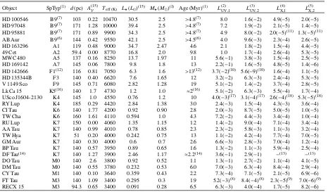
Table 5.Stellar parameters, and UV and X-ray irradiation properties, for 27 protoplanetary disks.
Object SpTyp(1) d(pc) A(15)
V Teff(K) L?(L)(15) M?(M)(1) Age (Myr)(1) L(2)UV,1 L(3)UV,2 L(4)X,1 L(5)X,2
HD 100546 B9(7) 103 0.22 10470 30.5 2.5 >4.8(7) 8.0 1.6(−2) 4.9(−5) 2.0(−5)
HD 97048 B9(7) 171 1.28 10000 39.4 2.5 >4.8(7) 7.2 1.9(−2) 2.1(−5) 1.4(−5)
HD 95881 B9(7) 171 0.89 9900 34.3 2.5 >4.8(7) 4.9 8.0(−2) 2.0(−5)(11) 1.3(−5)(11)
AB Aur B9(6) 144 0.42 9550 42.1 2.5 >4.5(6) 4.0 9.6(−3) 2.3(−4) 2.6(−5)
HD 163296 A1 119 0.48 9000 34.7 2.47 4.6 2.1 1.8(−2) 1.5(−4) 4.4(−5)
49 Cet A2 59.4 0.00 8770 16.8 2.0 9.8 1.0 1.7(−4) 2.6(−4) 5.3(−5)
MWC 480 A5 137 0.16 8250 13.7 1.97 11 5.6(−1) 3.8(−3) 1.5(−4) 2.5(−5)
HD 169142 A7 145 0.06 7800 9.8 1.8 13 2.2(−1) 1.6(−5) 4.8(−5) 1.4(−6)
HD 142666 F1(12) 116 0.81 7050 6.3 1.6 >13(12) 3.7(−2)(10) 5.6(−9)(10) 1.6(−4) 1.1(−5)
HD 135344B F3 140 0.40 6620 7.6 1.65 12 3.2(−2) 6.3(−3) 2.4(−4) 5.3(−5)
V 1149 Sco F9 145 0.71 6080 2.82 1.28 19 5.1(−2) 1.4(−2) 3.7(−4) 2.8(−5)
Lk Ca 15 K5(16) 140 1.7 4730 1.2 1.0 ≈2(16) 5.1(−2) 6.3(−3) 5.5(−4) 1.7(−4)
USco J1604-2130 K4 145 1.0 4550 0.76 1.2 10 4.0(−3)(17) 3.1(−4)(17) 2.6(−4)(18) 5.3(−5)(18)
RY Lup K4 185 0.29 4420 2.84 1.38 3.0 2.4(−3) 1.5(−4) 4.3(−3) 3.6(−4)
CI Tau K6 140 1.77 4200 0.92 0.90 2.8 2.0(−3) 8.7(−5) 5.0(−5) 1.0(−5)
TW Cha K6 160 1.61 4110 0.594 1.0 4.3 7.2(−2) 4.4(−3) 3.4(−4) 1.0(−4)
RU Lup K7 150 0.00 4060 1.35 1.15 1.2 1.4(−2) 9.0(−4) 7.1(−4) 3.4(−4)
AA Tau K7 140 0.99 4010 0.78 0.85 2.3 2.3(−2) 5.8(−3) 1.1(−3) 3.2(−4)
TW Hya K7 51 0.20 4000 0.242 0.75 13 1.1(−2) 4.2(−4) 7.7(−4) 7.0(−5)
GM Aur K7 140 0.30 4000 0.6 0.7 2.6 6.6(−3) 2.8(−3) 7.0(−4) 1.2(−4)
BP Tau K7 140 0.57 3950 0.89 0.65 1.6 1.3(−2) 1.1(−3) 5.9(−4) 2.5(−4)
DF Tau(14) K7 140 1.27 3900 2.46 1.17 ≈2.2(14) 3.6(−1) 2.9(−1) −(13) −(13)
DO Tau M0 140 2.6 3800 0.92 0.52 1.1 1.3(−1) 2.7(−2) 1.1(−4) 4.1(−5)
DM Tau M0 140 0.55 3780 0.232 0.53 6.0 7.0(−3) 6.3(−4) 8.4(−4) 2.9(−4)
CY Tau M1 140 0.10 3640 0.359 0.43 2.2 7.3(−4) 7.1(−5) 2.1(−5) 6.9(−6)
FT Tau M3 140 1.09 3400 0.295 0.3 1.9 5.2(−3)(8) 8.4(−4)(8) 2.3(−5)(9) 7.0(−6)(9)
RECX 15 M3 94.3 0.65 3400 0.091 0.28 6.5 6.3(−3) 4.0(−4) 1.7(−5) 8.2(−6)
Notes.The table shows spectral type, distanced, interstellar extinctionAV, effective temperatureTeff, stellar luminosityL?, stellar massM?, age,
and UV and X-ray luminosities without extinction, i.e. as seen by the disk. Numbers writtenA(−B) meanA×10−B. The UV and X-ray luminosities are listed in units of (L).(1)Spectral types, ages and stellar masses are consistent with evolutionary tracks for solar-metallicity premain sequence stars bySiess et al.(2000), usingTeff &L?as input,(2)FUV luminosity from 91.2 to 205 nm, as seen by the disk,(3)hard FUV luminosity from 91.2 to 111 nm, as seen by the disk,(4)X-ray luminosity for photon energies>0.1 keV, as seen by the disk,(5)hard X-ray luminosity from 1 keV
to 10 keV, as seen by the disk,(6)no matching track, values from closest point atT
eff = 9650 K andL? = 42L,(7)no matching track, values from closest point atTeff =10 000 K andL? =42L,(8)no UV data, model uses an UV-powerlaw with fUV =0.025 andpUV=0.2 (seeWoitke
et al. 2016)(9)no detailed X-ray data available, model uses a bremsstrahlungs-spectrum withL
X=8.8×1028erg s−1andTX =20 MK, based on
archival XMM survey data (M. Güdel, priv. comm.),(10)“low-UV state” model, where a purely photospheric spectrum is assumed,(11)no X-ray
data available, X-ray data taken from HD 97048,(12)no matching track, values from closest point atT
eff=7050 K andL?=7L,(13)no X-ray data available,(14)resolved binary, 2×spectral type M1, luminosities 0.69L
and 0.56L, separation 0.09400 ≈13 AU (Hillenbrand & White 2004),
(15)derived from fitting our UV, photometric optical and X-ray data(16)no matching track, values taken from (Drabek-Maunder et al. 2016;Kraus
et al. 2012),(17)no UV data, model uses f
UV=0.01 andpUV=2 (seeWoitke et al. 2016, Appendix A for explanations),(18)no X-ray data, model
usesLX=1030erg s−1andTX=20 MK (seeWoitke et al. 2016, Appendix A for explanations).
employed have been benchmarked for consistency (Woitke et al. 2016).
During the first modeling phase, additional photometric data are searched for, and initial values for e.g.,Teff, extinction,
dis-tance and luminosity values are looked up in previous spectral
analysis papers. The fitting is then made by varyingTeff,Lstarand
and log(g) are found by using stellar evolutionary tracks from Siess et al.(2000). In some cases it is necessary to connect the photospheric model with the UV observations by a power-law. In other cases (mostly for Herbig Ae stars) there is a good over-lap. Other groups proceed in a different way here, using early-type template spectra from selected sources, which have veiled pho-tospheric emission already built-in. During the first phaseMstar,
Lstar,Teff, log(g),AV, spectral type, distance and age are estimated as a result of the modeling process. However, initial values for a subset of these parameters can be collected from the rich literature which then are used as a starting point for the modeling (e.g., see TableC.2).
The second phase involves a collection of additional pho-tometric points, extending from the near IR to millimeter wavelengths, including far-IR lines fromHerscheland ISO. If polycyclic aromatic hydrocarbon (PAH) features are apparent in theSpitzer/IRS spectra, we include the PAH fitting (amount and average charge of PAHs) consistently in the SED fitting. As a result from the fitting process, the dust mass, disk size and shape, the dust settling and the dust-grain size parameters are constrained and if applicable, the amount and charge of PAHs. The result for 27 SED-fitted sources are included in the database and examples are presented in Fig.3.
In the third phase, line fluxes, line profiles, with resolved images from ALMA and NICMOS or visibility data from PIO-NIER and MIDI are included. The modeler decides which data to trust and which not (for example because the data is contaminated by backgroud or foreground cloud emission), assigns fitting weight to each observation, then follows the most appropriate fitting strategy, e.g., genetic fitting algorithm or by-hand-fitting. Fitting in phases two and three starts assuming a single-zone disk without gaps. If this fails, then a two-zone disk model is employed with a possible gap between the two zones. During the third phase, all phase 2 data refitted, where in particu-lar the radial extension, tapering parameters and shadow-casting from the inner to the outer zones can now be fitted using line observations, while the gas to dust ratio is constrained.
The methods are detailed inWoitke et al.(2016,2019), and the results are listed in Table5for 27 sources. The second step of the modeling is to determine the disk shape, dust and PAH properties by means of highly automated SED-fits. The result for 27 SED-fitted sources are included in the DIOD database and examples are presented in Fig.3.
4. Summary
In this paper we presented a large sample of Class II and III, T Tauri and Herbig Ae systems with spectral types ranging from B9 to M3 which cover ages between 1 and 10 Myr. The sample of 85 sources in expected to include another 30–40 sources in the near future, rendering this one of the largest and most complete collections of its kind. The collection was assembled combin-ing data from more than 50 observational facilities and 100 pub-lished articles in a transparent manner, so that each dataset can be back-traced to each original resources. In addition, 27 of the sources in the collection have their SEDs consistently modeled with dust radiative transfer models (MCFOST, MCMAX and ProDiMo)14, and a subset of 18 that have both dust and gas con-sistently modeled with ProDiMo15. The user interface and the
supporting DIOD database provide the user with the flexibility
14 All SED input files and output models available at: http://
www-star.st-and.ac.uk/~pw31/DIANA/SEDfit/
15 Gas line input files and output models available at: http://
www-star.st-and.ac.uk/~pw31/DIANA/DIANAstandard/
to compare different characteristics among the sample sources and models, but also directly download data for further use. We believe that this collection with its future extensions will provide a reference point, facilitating observational and modeling studies of protoplanetary disks.
Acknowledgements. The research leading to these results has received funding
from the European Union Seventh Framework Programme FP7-2011 under grant agreement no 284405. OD acknowledges support from the Austrian Research Promotion Agency (FFG) under the framework of the Austrian Space Appli-cations Program (ASAP) projects JetPro* and PROTEUS (854025, FFG-866005).
References
Adelman-McCarthy, J. K., Agüeros, M. A., Allam, S. S., et al. 2008,ApJS, 175, 297
Adelman-McCarthy, J. K. 2011,VizieR Online Data Catalog: II/306
Alecian, E., Wade, G. A., Catala, C., et al. 2013,MNRAS, 429, 1001
Ammons, S. M., Robinson, S. E., Strader, J., et al. 2006,ApJ, 638, 1004
Andre, P., & Montmerle, T. 1994,ApJ, 420, 837
Andrews, S. M., & Williams, J. P. 2007,ApJ, 671, 1800
Andrews, S. M., Czekala, I., Wilner, D. J., et al. 2010,ApJ, 710, 462
Ansdell, M., Williams, J. P., van der Marel, N., et al. 2016,ApJ, 828, 46
Antonellini, S., Kamp, I., Riviere-Marichalar, P., et al. 2015,A&A, 582, A105
Arnaud, K. A. 1996, in Astronomical Data Analysis Software and Systems V, eds. G. H. Jacoby, & J. Barnes,ASP Conf. Ser., 101, 17
Banzatti, A., Pontoppidan, K. M., Salyk, C., et al. 2017,ApJ, 834, 152
Beckwith, S. V. W., & Sargent, A. I. 1991,ApJ, 381, 250
Bergin, E. A., Cleeves, L. I., Gorti, U., et al. 2013,Nature, 493, 644
Bertout, C., Siess, L., & Cabrit, S. 2007,A&A, 473, L21
Biller, B., Lacour, S., Juhász, A., et al. 2012,ApJ, 753, L38
Bitner, M. A., Richter, M. J., Lacy, J. H., et al. 2008,ApJ, 688, 1326
Blake, G. A., & Boogert, A. C. A. 2004,ApJ, 606, L73
Boogert, A. C. A., Pontoppidan, K. M., Knez, C., et al. 2008,ApJ, 678, 985
Boss, A. P. 2009,ApJ, 694, 107
Bottinelli, S., Boogert, A. C. A., Bouwman, J., et al. 2010,ApJ, 718, 1100
Brown, J. M., Pontoppidan, K. M., van Dishoeck, E. F., et al. 2013,ApJ, 770, 94
Cabrit, S., Edwards, S., Strom, S. E., & Strom, K. M. 1990,ApJ, 354, 687
Calvet, N., Muzerolle, J., Briceño, C., et al. 2004,AJ, 128, 1294
Carmona, A., van den Ancker, M. E., Henning, T., et al. 2007,A&A, 476, 853
Carmona, A., van den Ancker, M. E., Henning, T., et al. 2008,A&A, 477, 839
Carmona, A., van der Plas, G., van den Ancker, M. E., et al. 2011,A&A, 533, A39
Carmona, A., Pinte, C., Thi, W. F., et al. 2014,A&A, 567, A51
Carpenter, J. M., Hillenbrand, L. A., Skrutskie, M. F., & Meyer, M. R. 2002,AJ, 124, 1001
Carpenter, J. M., Wolf, S., Schreyer, K., Launhardt, R., & Henning, T. 2005,AJ, 129, 1049
Chapillon, E., Guilloteau, S., Dutrey, A., Piétu, V., et al. 2008,A&A, 488, 565
Chen, H., Myers, P. C., Ladd, E. F., & Wood, D. O. S. 1995,ApJ, 445, 377
Cieza, L. A., Olofsson, J., Harvey, P. M., et al. 2013,ApJ, 762, 100
Cleeves, L. I., Bergin, E. A., Qi, C., Adams, F. C., & Öberg, K. I. 2015,ApJ, 799, 204
Cohen, M., Emerson, J. P., & Beichman, C. A. 1989,ApJ, 339, 455
Corradi, W. J. B., & Franco, G. A. P. 1995,A&AS, 112, 95
Cortes, S. R., Meyer, M. R., Carpenter, J. M., et al. 2009,ApJ, 697, 1305
Cutri, R. M. 2012,VizieR Online Data Catalog: II/311
Cutri, R. M., Skrutskie, M. F., van Dyk, S., et al. 2012,VizieR Online Data Catalog: II/281
Cutri, R. M., Skrutskie, M. F., van Dyk, S., et al. 2003,VizieR Online Data Catalog: II/246
Dent, W. R. F., Matthews, H. E., & Ward-Thompson, D. 1998,MNRAS, 301, 1049
Dent, W. R. F., Thi, W. F., Kamp, I., et al. 2013,PASP, 125, 477
Di Francesco, J., Johnstone, D., Kirk, H., MacKenzie, T., Ledwosinska, E., et al. 2008,ApJS, 175, 277
Donati, J.-F., Gregory, S. G., Montmerle, T., et al. 2011,MNRAS, 417, 1747
Drabek-Maunder, E., Mohanty, S., Greaves, J., et al. 2016,ApJ, 833, 260
Ducati, J. R. 2002,VizieR Online Data Catalog: II/237
Duchêne, G., McCabe, C., Pinte, C., et al. 2010,ApJ, 712, 112
Dutrey, A., Guilloteau, S., Duvert, G., et al. 1996,A&A, 309, 493
Egan, M. P., Price, S. D., Kraemer, K. E., et al. 2003,VizieR Online Data Catalog: V/114
ESA 1997, inThe Hipparcosand Tycho catalogues. Astrometric and Photometric Star Catalogues Derived from the ESA HipparcosSpace Astrometry Mission,
Espaillat, C., Calvet, N., D’Alessio, P., et al. 2007,ApJ, 670, L135
Evans, II., N. J., Allen, L. E., Blake, G. A., et al. 2003,PASP, 115, 965
Fedele, D., Bruderer, S., van Dishoeck, E. F., et al. 2013,A&A, 559, A77
Frasca, A., Biazzo, K., Lanzafame, A. C., et al. 2015,A&A, 575, A4
Fuente, A., Cernicharo, J., Agúndez, M., et al. 2010,A&A, 524, A19
Furlan, E., Luhman, K. L., Espaillat, C., et al. 2011,ApJS, 195, 3
Garufi, A., Benisty, M., Stolker, T., et al. 2017,The Messenger, 169, 32
Green, J. D., Yang, Y. L., & Evans, II., N. J. 2016,AJ, 151, 75
Grosso, N., Alves, J., Wood, K., et al. 2003,ApJ, 586, 296
Güdel, M., Briggs, K. R., Arzner, K., et al. 2007,A&A, 468, 353
Güdel, M., Lahuis, F., Briggs, K. R., et al. 2010,A&A, 519, A113
Guilloteau, S., Dutrey, A., Piétu, V., & Boehler, Y. 2011,A&A, 529, A105
Guilloteau, S., Dutrey, A., Wakelam, V., et al. 2012,A&A, 548, A70
Gullbring, E., Hartmann, L., Briceño, C., & Calvet, N. 1998,ApJ, 492, 323
Hauck, B., & Mermilliod, M. 1998,A&AS, 129, 431
Helou, G., & Walker, D. W. 1988, Infrared Astronomical Satellite (IRAS) Catalogs and Atlases. Volum e7: The Small Scale Structure Catalog, 7 Henning, T., Pfau, W., Zinnecker, H., & Prusti, T. 1993,A&A, 276, 129
Henning, T., Launhardt, R., Steinacker, J., & Thamm, E. 1994, in The Nature and Evolutionary Status of Herbig Ae/Be Stars, eds. P. S. The, M. R. Perez, & E. P. J. van den Heuvel,ASP Conf. Ser., 62, 171
Herczeg, G. J., & Hillenbrand, L. A. 2014,ApJ, 786, 97
Herczeg, G. J., Cruz, K. L., & Hillenbrand, L. A. 2009,ApJ, 696, 1589
Hillenbrand, L. A., & White, R. J. 2004,ApJ, 604, 741
Høg, E., Fabricius, C., Makarov, V. V., et al. 2000,A&A, 355, L27
Holmberg, J., Nordström, B., & Andersen, J. 2009,A&A, 501, 941
Howard, C. D., Sandell, G., Vacca, W. D., et al. 2013,ApJ, 776, 21
Hughes, J., Hartigan, P., Krautter, J., & Kelemen, J. 1994,AJ, 108, 1071
Humphries, C. M., Jamar, C., Malaise, D., & Wroe, H. 1976,A&A, 49, 389
Ida, S., & Lin, D. N. C. 2005,ApJ, 626, 1045
Ingleby, L., Calvet, N., Hernández, J., et al. 2011,AJ, 141, 127
Ingleby, L., Calvet, N., Herczeg, G., et al. 2013,ApJ, 767, 112
Isella, A., Carpenter, J. M., & Sargent, A. I. 2010,ApJ, 714, 1746
Ishihara, D., Onaka, T., Kataza, H., et al. 2010,A&A, 514, A1
Jansen, F., Lumb, D., Altieri, B., et al. 2001,A&A, 365, L1
Johns-Krull, C. M., Valenti, J. A., & Linsky, J. L. 2000,ApJ, 539, 815
Juhász, A., Bouwman, J., Henning, T., et al. 2010,ApJ, 721, 431
Kamp, I., Tilling, I., Woitke, P., Thi, W.-F., & Hogerheijde, M. 2010,A&A, 510, A18
Kamp, I., Thi, W.-F., Woitke, P., et al. 2017,A&A, 607, A41
Kharchenko, N. V. 2001,Kinematika i Fizika Nebesnykh Tel, 17, 409
Kimeswenger, S., Lederle, C., Richichi, A., et al. 2004,A&A, 413, 1037
Kitamura, Y., Momose, M., Yokogawa, S., et al. 2002,ApJ, 581, 357
Koerner, D. W., Chandler, C. J., & Sargent, A. I. 1995,ApJ, 452, L69
Kraus, A. L., & Hillenbrand, L. A. 2009,ApJ, 704, 531
Kraus, A. L., Ireland, M. J., Martinache, F., & Hillenbrand, L. A. 2011,ApJ, 731, 8
Kraus, A. L., Ireland, M. J., Hillenbrand, L. A., & Martinache, F. 2012,ApJ, 745, 19
Lahuis, F., van Dishoeck, E. F., Blake, G. A., et al. 2007,ApJ, 665, 492
Laughlin, G., Bodenheimer, P., & Adams, F. C. 2004,ApJ, 612, L73
Lebouteiller, V., Barry, D. J., Spoon, H. W. W., et al. 2011,ApJS, 196, 8
Lebreton, J., Augereau, J.-C., Thi, W.-F., et al. 2012,A&A, 539, A17
Lommen, D., Wright, C. M., Maddison, S. T., et al. 2007,A&A, 462, 211
Lommen, D., Maddison, S. T., Wright, C. M., et al. 2009,A&A, 495, 869
Luhman, K. L. 2007,ApJS, 173, 104
Luhman, K. L., Allen, P. R., Espaillat, C., Hartmann, L., & Calvet, N. 2010,
ApJS, 186, 111
Manara, C. F., Testi, L., Natta, A., et al. 2014,A&A, 568, A18
Mannings, V. 1994,MNRAS, 271, 587
Mannings, V., & Emerson, J. P. 1994,MNRAS, 267, 361
Manset, N., Bastien, P., Ménard, F., et al. 2009,A&A, 499, 137
Martin-Zaïdi, C., Augereau, J.-C., Ménard, F., et al. 2010,A&A, 516, A110
Mathews, G. S., Dent, W. R. F., Williams, J. P., et al. 2010,A&A, 518, L127
Mathews, G. S., Williams, J. P., & Ménard, F. 2012,ApJ, 753, 59
Mathews, G. S., Pinte, C., Duchêne, G., Williams, J. P., & Ménard, F. 2013,
A&A, 558, A66
Matthews, B. C., Kalas, P. G., & Wyatt, M. C. 2007,ApJ, 663, 1103
McJunkin, M., France, K., Schneider, P. C., et al. 2014,ApJ, 780, 150
Meeus, G., Waters, L. B. F. M., Bouwman, J., et al. 2001,A&A, 365, 476
Meeus, G., Montesinos, B., Mendigutía, I., et al. 2012,A&A, 544, A78
Meeus, G., Salyk, C., Bruderer, S., et al. 2013,A&A, 559, A84
Mendigutía, I., Mora, A., Montesinos, B., et al. 2012,A&A, 543, A59
Mendigutía, I., Fairlamb, J., Montesinos, B., et al. 2014,ApJ, 790, 21
Mermilliod, J. C. 2006,VizieR Online Data Catalog: II/168
Mermilliod, J.-C., Mermilliod, M., & Hauck, B. 1997,A&AS, 124, 349
Meyer, M. R., Hillenbrand, L. A., Backman, D., et al. 2006, PASP, 118, 1690
Min, M., Dullemond, C. P., Dominik, C., de Koter, A., & Hovenier, J. W. 2009,
A&A, 497, 155
Monet, D. G., Levine, S. E., Canzian, B., et al. 2003,AJ, 125, 984
Montesinos, B., Eiroa, C., Mora, A., & Merín, B. 2009,A&A, 495, 901
Morel, M., & Magnenat, P. 1978,A&AS, 34, 477
Morrison, R., & McCammon, D. 1983,ApJ, 270, 119
Morrissey, P., Conrow, T., Barlow, T. A., et al. 2007,ApJS, 173, 682
Moshir, M. 1990,IRAS Faint Source Catalogue, version 2.0 (1990)
Motte, F., Andre, P., & Neri, R. 1998,A&A, 336, 150
Murakami, H., Baba, H., Barthel, P., et al. 2007,PASJ, 59, 369
Najita, J., Carr, J. S., & Mathieu, R. D. 2003,ApJ, 589, 931
Nilsson, R., Liseau, R., Brandeker, A., et al. 2009,A&A, 508, 1057
Nuernberger, D., Chini, R., & Zinnecker, H. 1997,A&A, 324, 1036
Öberg, K. I., Boogert, A. C. A., Pontoppidan, K. M., et al. 2008,ApJ, 678, 1032
Öberg, K. I., Qi, C., Fogel, J. K. J., et al. 2010,ApJ, 720, 480
Öberg, K. I., Qi, C., Fogel, J. K. J., et al. 2011,ApJ, 734, 98
Ofek, E. O. 2008,PASP, 120, 1128
Osterloh, M., & Beckwith, S. V. W. 1995,ApJ, 439, 288
Palla, F., & Stahler, S. W. 2002,ApJ, 581, 1194
Pascucci, I., Apai, D., Luhman, K., et al. 2009,ApJ, 696, 143
Perryman, M. A. C., Lindegren, L., Kovalevsky, J., et al. 1997,A&A, 323, L49
Pickles, A., & Depagne, É. 2010,PASP, 122, 1437
Pinte, C., Harries, T. J., Min, M., et al. 2009,A&A, 498, 967
Pinte, C., Ménard, F., Duchêne, G., & Bastien, P. 2006,A&A, 459, 797
Pontoppidan, K. M., Boogert, A. C. A., Fraser, H. J., et al. 2008,ApJ, 678, 1005
Pontoppidan, K. M., Salyk, C., Blake, G. A., et al. 2010,ApJ, 720, 887
Pontoppidan, K. M., van Dishoeck, E., Blake, G. A., et al. 2011,The Messenger, 143, 32
Rebull, L. M., Padgett, D. L., McCabe, C.-E., et al. 2010,ApJS, 186, 259
Rebull, L. M., Koenig, X. P., Padgett, D. L., et al. 2011,VizieR On-line Data Catalog: J/ApJS/196/4
Ricci, L., Testi, L., Natta, A., et al. 2010,A&A, 512, A15
Rice, W. K. M., & Armitage, P. J. 2009,MNRAS, 396, 2228
Richmond, M. W. 2007,PASP, 119, 1083
Roberge, A., Kamp, I., Montesinos, B., et al. 2013,ApJ, 771, 69
Rodmann, J., Henning, T., Chandler, C. J., Mundy, L. G., & Wilner, D. J. 2006,
A&A, 446, 211
Rufener, F. 1988, Catalogue of Stars Measured in the Geneva Observatory Photometric System, 4, 1988
Sacco, G. G., Flaccomio, E., Pascucci, I., et al. 2012,ApJ, 747, 142
Salyk, C., Pontoppidan, K. M., Blake, G. A., Najita, J. R., & Carr, J. S. 2011,
ApJ, 731, 130
Salyk, C., Herczeg, G. J., Brown, J. M., et al. 2013,ApJ, 769, 21
Sandell, G., Weintraub, D. A., & Hamidouche, M. 2011,ApJ, 727, 26
Sartori, M. J., Lépine, J. R. D., & Dias, W. S. 2003,A&A, 404, 913
Schaefer, G. H., Dutrey, A., Guilloteau, S., Simon, M., & White, R. J. 2009,ApJ, 701, 698
Schindhelm, E., France, K., Herczeg, G. J., et al. 2012,ApJ, 756, L23
Siess, L., Dufour, E., & Forestini, M. 2000,A&A, 358, 593
Skiff, B. A. 2014,VizieR Online Data Catalog: B/mk
Smith, B. J., Price, S. D., & Baker, R. I. 2004,ApJS, 154, 673
Spitzer Science 2009,VizieR Online Data Catalog: II/293
Stark, C. C., Schneider, G., Weinberger, A. J., et al. 2014,ApJ, 789, 58
Straizys, V., Kazlauskas, A., Jodinskiene, E., & Bartkevicius, A. 1989,Bulletin d’Information du Centre de Données Stellaires, 37, 179
Testi, L., Natta, A., Shepherd, D. S., & Wilner, D. J. 2003,A&A, 403, 323
Thi, W.-F., Woitke, P., & Kamp, I. 2011,MNRAS, 412, 711
Torres, C. A. O., Quast, G. R., da Silva, L., et al. 2006,A&A, 460, 695
Trotta, F., Testi, L., Natta, A., Isella, A., & Ricci, L. 2013,A&A, 558, A64
Ubach, C., Maddison, S. T., Wright, C. M., et al. 2012,MNRAS, 425, 3137
Valenti, J. A., Johns-Krull, C. M., & Linsky, J. L. 2000,ApJS, 129, 399
Valenti, J. A., Fallon, A. A., & Johns-Krull, C. M. 2003,ApJS, 147, 305
van der Wiel, M. H. D., Naylor, D. A., Kamp, I., et al. 2014,MNRAS, 444, 3911
Verhoeff, A. P., Min, M., Pantin, E., et al. 2011,A&A, 528, A91
Wahhaj, Z., Cieza, L., Koerner, D. W., et al. 2010,ApJ, 724, 835
Weisskopf, M. C., Tananbaum, H. D., Van Speybroeck, L. P., O’Dell, S. L., et al. 2000, in X-Ray Optics, Instruments, and Missions III, eds. J. E. Truemper, & B. Aschenbach,SPIE Conf. Ser., 4012, 2
Wesselius, P. R., van Duinen, R. J., de Jonge, A. R. W., et al. 1982,A&AS, 49, 427
White, R. J., & Hillenbrand, L. A. 2004,ApJ, 616, 998
Woitke, P., Kamp, I., Antonellini, S., et al. 2019,PASP, 131, 1000
Woitke, P., Kamp, I., & Thi, W.-F. 2009,A&A, 501, 383
Woitke, P., Min, M., Pinte, C., et al. 2016,A&A, 586, A103
Yang, H., Herczeg, G. J., Linsky, J. L., et al. 2012,ApJ, 744, 121
Yokogawa, S., Kitamura, Y., Momose, M., et al. 2001,ApJ, 552, L59
Appendix A: The DiscAnalysis Object Database (DIOD)
The multiwavelength datasets available through the DIANA
Object Database repository are processed end-products, as
opposed to raw data, that can be directly compared to models. Deriving meaningful physical quantities from raw astrophysical data is a complex process that requires good knowledge of the instrumentation involved, together with adequate experience and advanced programing skills. Therefore the dissemination of pro-cessed end-products has a greater impact to the community as they can be directly used for analysis and interpretation. As an example we mention the SDSS survey that has been up to now the most prolific project in terms of scientific outcome when compared to cost. We therefore anticipate that along with the advancements and increasing interest in the field, our database will become a point of reference for the study of protoplanetary disks.
A.1. The end-user interface
The database functionalities for the end-user are limited to searching, inspecting and downloading datasets and models for either single or multiple sources.
When the Download window is selected in the welcome page, the user is redirected to the data search and retrieval inter-face. As in most pages of the interface, a short description of the available functions are displayed on the top part. At this stage the user is provided with two options: either search for a source by name, or select sources from a list that is returned when the
List all objectsbutton is selected (Fig.A.1). In the list window,
presented in Fig.A.2the user can search the database for alter-native source names as provided by online name resolvers. In addition, selection of a source name brings into the foreground a pop-up window, which provides detailed information on the source as retrieved by the SIMBAD, NED and VizieR and CDS name servers (Fig.A.3).
Once one or more sources are selected, they appear on the right panel of the search and retrieval window (Fig.A.6), under
the Selected Objectssection. At the same section, sources can
be removed by selecting the “X” symbol next to each source name. Below theSelect functionpane, two lists appear provid-ing the possibility to select first theData Type(e.g., photometric points, spectra, line fluxes, line shapes, etc). For each data type,
theDatasetbox is populated with available options (instruments,
bands, etc). Information on all selected datasets is listed below under the pane bearing the same title. Here, the user can find information on the original source where the data is retrieved from and an active link to the original publication (if available). In addition, the user is informed on the data quality by rele-vant flags and comments on the data. Comments are truncated to save space, but the full comments are displayed once the user “hoovers over” the mouse pointer.
A.2. Data preview and retrieval
[image:12.595.322.541.82.169.2]Selected datasets can be previewed and compared on the plotting window. Once desired datasets or models are selected for one or more sources they are plotted using a color-encoded scheme that allows to distinguish the data origin into individual sources, datasets and instruments. For a “mouse-over” action a pop-up window displays the provenance of the specific data point (see Fig.A.5). When the full screen plotting mode is selected, then a complete list on the provenance of all data points is provided on
Fig. A.1.The data search and download window, without any sources
[image:12.595.324.538.229.402.2]selected. The user can either search for a source by its name, or get a list of all available sources when selecting theList all sourcesbutton.
Fig. A.2.List of available sources that can be selected for further
inves-tigation and download by marking the checkbox on theright of the
source name. On thetopthe user can search the source list with alter-native names, as provided by source name resolvers. Direct selection of a source name presents information retrieved by three online name resolver services (see Fig.A.3).
Fig. A.3.When selecting a source, a pop-up window presents its details
as retrieved from SIMBAD, NED and VizieR and CDS name resolvers.
[image:12.595.322.542.489.656.2]