Distractor-aware deep regression for visual tracking

(1)

White Rose Research Online URL for this paper:

http://eprints.whiterose.ac.uk/141207/

Version: Published Version

Article:

Du, M., Ding, Y., Meng, X. et al. (2 more authors) (2019) Distractor-aware deep regression

for visual tracking. Sensors, 19 (2). 387. ISSN 1424-8220

https://doi.org/10.3390/s19020387

[email protected] https://eprints.whiterose.ac.uk/ Reuse

This article is distributed under the terms of the Creative Commons Attribution (CC BY) licence. This licence allows you to distribute, remix, tweak, and build upon the work, even commercially, as long as you credit the authors for the original work. More information and the full terms of the licence here:

https://creativecommons.org/licenses/

Takedown

If you consider content in White Rose Research Online to be in breach of UK law, please notify us by

(2)

Article

Distractor-Aware Deep Regression for

Visual Tracking

Ming Du1 , Yan Ding1,* , Xiuyun Meng1, Hua-Liang Wei2 and Yifan Zhao3

1 _{Key Laboratory of Dynamics and Control of Flight Vehicle, Ministry of Education, School of Aerospace}

Engineering, Beijing Institute of Technology, Beijing 100081, China; [email protected] (M.D.); [email protected] (X.M.)

2 _{Department of Automatic Control and Systems Engineering, University of Sheffield, Sheffield S1 3JD, UK;}

[email protected]

3 _{Through-Life Engineering Services Institute, School of Aerospace, Transport and Manufacturing,}

Cranfield University, Cranfield, Bedfordshire MK43 0AL, UK; [email protected]

* Correspondence: [email protected]

Received: 2 December 2018; Accepted: 15 January 2019; Published: 18 January 2019

Abstract:In recent years, regression trackers have drawn increasing attention in the visual-object

tracking community due to their favorable performance and easy implementation. The tracker algorithms directly learn mapping from dense samples around the target object to Gaussian-like soft labels. However, in many real applications, when applied to test data, the extreme imbalanced distribution of training samples usually hinders the robustness and accuracy of regression trackers. In this paper, we propose a novel effective distractor-aware loss function to balance this issue by highlighting the significant domain and by severely penalizing the pure background. In addition, we introduce a full differentiable hierarchy-normalized concatenation connection to exploit abstractions across multiple convolutional layers. Extensive experiments were conducted on five challenging benchmark-tracking datasets, that is, OTB-13, OTB-15, TC-128, UAV-123, and VOT17. The experimental results are promising and show that the proposed tracker performs much better than nearly all the compared state-of-the-art approaches.

Keywords:object tracking; deep-regression networks; data imbalance; distractor aware

1. Introduction

Visual-object tracking aims to estimate the trajectory of the specified target in a video sequence, which is labeled in the initial frame with a bounding box. It is widely used in various applications, ranging from video surveillance, motion analysis, and autonomous driving. The main difficulty of visual tracking is how to accurately and effectively locate the object in challenging scenarios caused by illumination, deformation, occlusion, out of view, background cluttering, and other variations [1–3].

Modern tracking methods can be classified as either generative or discriminative. Generative methods aim at describing the target appearance using some generative processes (e.g., statistical models [4], templates [5], or sparse coding [6–10]), and searching the candidates to minimize reconstruction errors. Discriminative approaches instead regard tracking as a classification problem by differentiating target appearance and the surrounding background. Numerous classifiers have been introduced in the tracking community, such as structured support vector machine [11,12], boosting [13], oblique random forests [14], and online multiple-instance learning [15]. Recently, discriminative correlation filters (DCF) trackers [16–25], which directly regress the dense samples to soft labels, have sparked significant attention due to their high accuracy and efficiency. Furthermore, the favorable performance of deep convolutional networks on several challenging vision tasks [26–28] encourages

(3)

recent works to either exploit existing deep convolutional-neural-network (CNN) features within discriminative correlation filters [29–33], or design deep architectures [34–40] for discriminative visual tracking.

Despite top performance on benchmarks, discriminative correlation filters take few advantages of end-to-end training. On the contrary, deep regression networks that reformulate the correlation operation as a convolutional layer are fully differentiable and can be trained end to end. In this paper, we show that a deep regression tracker, when properly designed, can achieve even better and competitive results compared with the state-of-the-art trackers, especially with discriminative correlation filters. A critical issue relating to deep regression trackers is the data-imbalance problem [39,41,42] where the number of samples in the negative class is large but it is much smaller in the positive class. It is known that “easy” negative samples dominate the training dataset, and this inevitably suppresses the contribution of positive samples and therefore affects the performance of the resulting regression networks. In addition, distractor samples whose semantic abstraction close to the target may also be suppressed despite having an important contribution to model robustness. The existing approaches to dealing with data imbalance in regression trackers mainly focus on reducing the role and influence of background samples and pay little attention to the contribution of semantic distractors. In this work, we try to address the imbalance-distribution issue by introducing a novel distractor-aware loss function during the learning of the regression networks. The proposed distractor-aware loss function differs from existing approaches (e.g., shrinkage loss [39] and focal loss [43]) in that our approach barely utilizes easy negative samples and increase the importance of distractor samples (see Section3.2), whereas shrinkage loss only penalizes easy samples and focal loss partially reduces the importance of hard samples.

To further promote the performance of deep feature-based trackers, many efforts have been made in the visual-object tracking communities. Leveraging multilevel semantic abstraction exploitation across multiple convolutional layers has drawn more and more attention. Residual connections across multiple convolutional layers can mine distinguished information compared with independently learning on multiple convolutional layers. However, residual connected regression networks will become massive when the across-number of convolutional layers increases. Furthermore, the lack of training data often makes the regression networks unable to effectively balance the numerical values of multi-layer features. In this work, we propose to apply hierarchy-normalized concatenation to fuse multiple convolutional layers. The proposed scheme, with a simple structure and without numerical issue, can make full use of multi-level convolutional features across multiple convolutional layers. By taking advantage of distractor-aware loss and hierarchy-normalized concatenation, the proposed tracking method achieves favorable results against the state-of-the-art trackers on several tracking benchmarks.

The main contributions of this work can be summarized as three parts:

1. The proposed novel distractor-aware loss can alleviate the data-imbalance issue in learning deep-regression networks. We observe that the adversarial semantic distractors not only facilitate robustness in the tracking phrase but also accelerate convergence in the training phrase.

2. We leveraged hierarchy-normalized concatenation to fully exploit multilevel semantic abstraction across multiple convolutional layers. This results in a simple and easy-to-train end-to-end regression network for visual tracking.

(4)

2. Related Work

Visual tracking has long been an active research topic with extensive surveys and benchmark evaluations. In this section, we give a brief review on most relevant tracking approaches and pay attention to the data-imbalance issue. Comprehensive reviews on object tracking can be found in References [2,44,45].

2.1. Trackers with Correlation Filters

Correlation filters have recently attracted considerable attention in the object-tracking community due to their high computational efficiency and favorable robustness. Trackers based on correlation filters regress all circular-shifted versions of input samples to Gaussian-like soft labels. Bolme et al. [46] proposed to exploit the correlation filters for visual tracking and optimized the output sum of squared errors in the Fourier domain, leading to an extremely fast tracker at 669 frames per second (FPS). Henriques et al. [16] first suggested to regress all circular shifted versions of illumination-intensity features to a Gaussian label. Furthermore, Henriques et al. [17] incorporated kernel functions into the correlation filter and extended the correlation filters to multiple channel histograms of gradient (HOG) features. Inspired by the work of Reference [16], several extensions have been proposed to promote the accuracy and robustness of correlation filter-based trackers. Extensions include, but are not limited to, kernelized correlation filters [17,47], scale estimation [19,48], redetection [24], spatial regularization [20–22,31], context learning [23,49] and CNN feature integrations [29,32,33,50].

2.2. Trackers with Deep Regression

Benefiting from the strong representation of CNN features, correlation filter-based trackers have achieved distinguishable performance. However, associated optimization in Fourier domain suffers the boundary effect. Different from traditional correlation filter-based trackers, deep-regression trackers try to obtain an approximate solution via gradient descent in spatial domain. They formulate the correlation filter as a convolution operation and build a one-channel-output convolution layer, as used in a typical convolutional neural network. Recent trackers [35,38,39,41] follow this manner and achieve significant improvement in performance on par with correlation-filter trackers. Chen et al. [41] introduced a single-layer regression model for visual tracking and exploited a novel automatic hard-negative mining method to facilitate training the regression model. Wang et al. [35] introduced a fully convolutional network to exploit multiple CNN features by leveraging a feature-map selection strategy. Both a top layer and a lower layer were jointly used with a switch mechanism during tracking. Song et al. [38] proposed to apply residual learning to take appearance changes into account on a single convolutional layer, and formulated the tracking progress in an end-to-end manner by integrating feature extraction, response-map generation, and model updates into the neural networks. Lu et al. [39] proposed to apply residual connections to fuse two convolutional layers as well as their output response maps, achieving remarkable results. However, we observed that residual connections across multiple layers are more or less suffering from the numerical-imbalance issue (see Section3.3). In order to tackle the numerical-imbalance issue, we propose to apply a hierarchy-normalized concatenation operation to directly connect multiple convolutional layers. The novel connection is fully differential and can make the network more concise.

2.3. Data Imbalance

(5)

mining method to eliminate easy negatives and enhance positives. A recent work [43] on dense-object detection proposed focal loss to decrease loss from easy samples as well as partially decrease the loss of hard samples. Song et al. [42] proposed to apply cost-sensitive loss to decrease the effect from easy negatives. Lu et al. [39] exploited shrinkage loss to penalize the loss from easy samples, and kept the hard samples unchanged. Unlike the aforementioned solutions for the data-imbalance issue, we propose a distractor-aware loss to adaptively reinforce significant semantics and extremely penalize a pure background. This scheme improves both tracking accuracy and robustness, and accelerates training convergence.

3. Proposed Algorithm

The proposed Distractor-aware Deep Regression Tracking (DaDRT) algorithm follows a general one-channel-output regression framework. In addition, we exploit a novel distractor-aware loss function to handle data imbalance and introduce a hierarchy-normalized concatenation connection to fully exploit multilevel semantics across convolutional layers. Figure1shows an overview of our pipeline. Details are discussed below.

C

Conv5 Conv4

[image:5.595.157.442.305.471.2]

Conv3 Conv2 Conv1

Figure 1.Overview of the proposed deep regression network. The left-side blocks are the fixed-feature extractor backbone. The right-side blocks are trained in the first frame and updated frame by frame.

The blue blocks represent the 1×1 channel reduction layers, and red blocks represent the normalization

and rescale layers. The yellow block indicates the target-specified one-channel-output convolutional regression layer. The connection circle means hierarchy concatenation. The proposed network effectively exploits semantic abstraction across three convolutional layers.

3.1. Regression via Convolution Layer

The regression model for visual tracking aims to regress dense samples to Gaussian-like soft labels. Here, we revisit the linear-ridge regression model and formulate the regression model as one convolutional layer. Given an initial image with labeled target, we can extract dense sample features

X, and generate corresponding Gaussian function labelsY. The coefficientsWfor regression function

f=X∗Ware estimated by solving the following minimization problem:

min

W {kW∗X−Yk

2

2+λkWk22} (1)

where∗denotes the convolution operation, andλis a regularization parameter that controls overfitting. Particularly, there exists a closed-form solution for this problem by transforming the convolution operation between coefficientsWand samplesXinto an elementwise product in the Fourier domain. Here, we try to solve the regression problem in the spatial domain by reformulating the problem as loss minimization of the convolutional neural network.

(6)

L(W) =kF(W,X)−Yk2₂+λkWk2₂ (2)

whereF(W,X) =W∗Xis the network output,Wis the network weights, andYis the ground-truth labels. The convolution operation onXcan be carried out via a convolution layer with one-channel output. The size of the convolution kernel in the regression layer is different from conventional convolution layers that adopt a small fixed receptive field, such as 3 × 3 and 5 × 5. We set the receptive-field size of the regression layer to the size of a tracked target in our framework. The convolutional weights can be effectively calculated by iteratively optimizingWin Equation (2) using the gradient descent method, which can be implemented in almost all modern deep-learning frameworks. Regularization parameterλ is usually explained as weight decay in deep-learning frameworks. In this study, the value of parameterλis determined by following the default setting in the implemental platform.

3.2. Distractor-Aware Loss

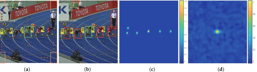
For deep-regression tracking, it is possible to exploit all real extracted samples by sliding a window fashion over the whole image during the training and detecting stages. The region of interest (ROI) contains a large amount of context surrounding the target object, as shown in Figure2a. The large surrounding context contains a majority of pure background and few semantic distractors, as shown in Figure2b. A large amount of background helps strengthen the discriminative power of the target object from the background, and distractors help discriminate the target object from a similar context. However, this also leads to an increase in the number of easy negative samples. Reviewing Equation (2), when summed over the large input search area, the loss values from easy negative samples submerge the valuable and rare positive samples and distractors. The learning progress usually drifts to a classification problem between objects and backgrounds due to the easy negative samples dominating the gradient. The tracker is less robust to similar semantic distractors.

(a) (b)

0 0.2 0.4 0.6 0.8 1 1.2 1.4 1.6 1.8

(c)

0 0.2 0.4 0.6 0.8 1

[image:6.595.82.524.444.568.2]

(d)

Figure 2.(a) Sliding sampled region of interest (ROI) centered on the target. (b) Obvious semantic

distractors labeled in red bounding boxes. (c) Modulating factor in one training epoch. Note that the

easy background is extremely suppressed, and the target and several selected distractors are reinforced.

(d) Output regression map of the regression network.

Existing solutions to the data-imbalance issue mainly focus on penalizing the importance of easy negative samples. However, we observed that semantic distractors have a significant contribution in learning deep-regression networks. We propose to add a modulating factor to the loss that highly suppresses pure backgrounds and protrudes the target and semantic distractors, as shown in Figure2c. Formally, we formulate our distractor-aware loss function as:

L(W) =D⊙ kF(W,X)−Yk2

2+λkWk22 (3)

(7)

optimization iteration. We denote the regression network output in every iteration byR, which generally indicates the probability of a position to be the target object. Once we obtained the probability map, we first identitied a number ofNsemantic objects by locating the local maximum ofR. In general, there is always one positive sample at the map center andNminus one distributed negative distract samples. For each semantic sample, we generated a basic modulatorDb in terms of soft labelsY

centered at the identified positions:

Db=Y⊙ek(Y−1) (4)

wherekis a scalar penalization factor. ModulatorDbaims at highlighting the central influence and

suppressing the surrounding influence. Then, we merged theNbasic modulators by summation. In addition, we took one more modulator on the target location to increase the importance of positive samples. Figure2c illustrates a modulating factor in the training iteration. Note that, in comparison with general deep-regression trackers, the proposed loss function introduces two extra hyperparameters, that is,kandN. We observed that the larger the value ofkwas, the larger the penalty to the surrounding contexts. A largerNmeans taking more distractors to take into account, which may overwhelm the only positive sample. On the other hand, a smallerNmakes the training process overfit to the target. Considering the proportion of positive and distractor samples, we fixed thek = 1.6 and the number of semantic objectsNto be 6 in all our experiments, meaning we introduced five adversarial distractors to go against the positive sample.

By applying the modulating factor, distractor-aware loss mainly focuses on positive samples and adversarial distractors. Extensive comparison with other losses shows that our distractor-aware loss not only promotes tracking accuracy but also accelerates training speed (see Section5.3).

3.3. Hierarchy-Normalized Concatenation

The convolutional layers of a typical CNN model, e.g., VGG [28], provide different levels of semantic abstraction in the features hierarchies. Features in the earlier layers, with higher spatial details, are helpful in precise localization; features in the later layers capture more semantic abstraction and are robust to large appearance changes. Motivated by this observation, many efforts have been made to exploit the merits of multiple convolutional layers, including independent learning [32,35] and residual connection [38,39]. Danelljan et al. [32] proposed to independently learns correlation filters over theconv1andconv5layers and merges the corresponding output response maps with empirical weights. Wang et al. [35] proposed to independently exploit two branch networks on theconv4and

conv5layers, and merge the output response map with a distractor-detection scheme. Song et al. [38] proposed to apply residual connections on a singleconv4layer to capture the difference between the base layer output and the ground truth. Lu et al. [39] exploited the residual connections to fuseconv4

andconv5layers as well as their output response maps. Here, we propose a novel hierarchy-normalized concatenation connection to make full use of multiple-level semantic abstraction. We introduced a normalize operation to balance the features’ numeric value and then concatenated theconv3,conv4, andconv5layers to form a strong representation for visual tracking. We compare our scheme with the aforementioned connections in Figure3.

(8)

importance of feature channels. Our connection scheme not only jumps out the weight-initialization straits but also permits a higher learning rate in regression training, which accelerates convergence.

[image:8.595.93.498.131.210.2]

Response Conv Feature-1 Response Conv Feature-2 Prediction Response Feature-1 Response Corr.Filter Feature-2 Prediction Corr.Filter 1 Adjust Feature-1 Adjust Feature-2 C Prediction Conv 2 3 ours

Figure 3. Three types of feature connection. (1) Independent connection that is used in traditional

correlation-filter trackers (e.g., ECO [32]). Pediction is obtained by weighted summing from different

correlation-filter responses. (2) By substituting a traditional correlation filter with a convolutional layer,

the second type can exploit various end-to-end residual connections. CREST [38] exploits only a single

convolutional layer (conv4_3fromVGG16) that meansfeature-1andfeature-2are the same to form a base

and a residual network. The DSLT [39] leverages two convolutional layers (conv4_3andconv5_3from

VGG16) to learn the residual across multiple convolutional layers. (3) Our scheme exploits the feature

adjuster (normalization) to fuse multiple convolutional layers. We learn a regression layer directly on the reinforced feature represented. The proposed scheme can easily incorporate more features without increasing the convolutional parameters.

0 50 100 150 200 250 300

0 200 400 600 800 1000

1200 Average of each channel on conv3_3

bolt bird2

0 50 100 150 200 250 300

0 500 1000

1500 Standard deviation of each channel on conv3_3

bolt bird2

0 50 100 150 200 250 300

0 2000 4000 6000 8000 10000 12000 14000 16000

18000 Maximum element of each channel on conv3_3

bolt bird2

0 100 200 300 400 500 600

0 20 40 60 80 100 120 140 160 180

bolt bird2

0 100 200 300 400 500 600

0 500 1000 1500 2000 2500 3000

bolt bird2

0 100 200 300 400 500 600

0 50 100 150 200 250 300

bolt bird2

0 100 200 300 400 500 600

0 1 2 3 4 5 6 7 8

bolt bird2

0 100 200 300 400 500 600

0 50 100 150 200

bolt bird2

0 100 200 300 400 500 600

0 5 10

bolt bird2

Figure 4. Visualizations of numeric distribution at different abstraction levels on two sequences.

High-level abstractions (bottomrow) emerge with smaller values compared with low-level abstractions

(toprow). It is unreasonable to directly add the features of different convolutional layers together.

[image:8.595.95.502.350.697.2]

(9)

4. Tracking via DaDRT

We illustrate the detailed procedure of DaDRT for visual tracking. We decomposed our tracking process into four stages, namely, model initialization, online detection, scale estimation, and model update. Details are as follows:

• Model Initialization. At this stage, we follow the general tracking initialization process [17,32,38]

to locate the target of interest as suggested by the benchmark [1–3,57,58]. In initial frame

I0, the target state is usually given by a bounding boxbb0 = {x0,y0,w0,h0}, where {x0,y0}

denotes the left-top pixel position and{w0,h0}indicates the target width and height respectively.

We leveraged a new bounding boxcp0={x0+ (1−cx)w0/2, y0+ (1−cy)h0/2, cxw0, cyh0}to

crop the sample patch for tracking initialization, where scalarscxandcydenote amplification

factors; in this study, we suggestcx = 5,cy = 9. Especially for the unbalanced target-aspect

ratio, we fixed the amplification factor of the long side to 5, and a larger amplification to the short side to keep the bounding box squarelike. Once the sample patch is acquired, we adopt the tailoredVGG16network as the backbone-feature extractor and feed the sample patch into the extractor. Then, we take the output of theconv3_3,conv4_3, andconv5_3layers as deep features for further training the regression network. The data flow is illustrated in Figure1. Meanwhile, all parameters in the regression layers are randomly initialized following the improved Xavier [59] method. The regression layers are well-initialized after a number of training steps.

• Online Detection. For current frame It, the previous predicted target state bbt−1 =

{xt−1,yt−1,wt−1,ht−1}is utilized to derive the search patch bounding boxcpt = {xt−1+ (1−

cx)wt−1/2, yt−1+ (1−cy)ht−1/2, cxwt−1, cyht−1}. The search patch is cropped according to

bounding boxcptand is delivered to the designed network to generate a response map. Motion

constraint is further introduced to increase the robustness. We leverage an isotropy Gaussian function to produce motion constraint map that penalizes large deviation away from the previous target location. We carry out the prediction map by elementwise multiplying the motion map with the response map. Once we obtain the prediction map, we predict the target object by locating the maximum prediction value.

• Scale Estimation. After obtaining the target position in the current frame, we extract scale search

patches following the scale pyramid scheme as in ACF [48]. We generate the scale response map by feeding these scale search patches into our regression network. The index of maximum response indicates the current scale location. Then, we update the target scale by a smooth manner:

(wt,ht) =β(wp∗,hp) + (1−β)(wt−1,ht−1) (5)

wherewtandhtrepresent the width and height of the target object at framet, respectively; and

wp,hpare the predicted width and height from the detection scheme. Scalar weightβenables a smooth update of the target scale.

• Model Update. In order to accommodate the model to the varied object appearance,

we incrementally update our tracker frame by frame. For each frame, we crop the training patch relying on the estimated location and scale and generate corresponding soft labels. To alleviate model drift from noisy updates, training data pairs from pastT frames are all adopted for online update.

5. Experiments

(10)

5.1. Implementation Setup

We implement the proposed DaDRT in Matlab using the matconvnet toolbox [60]. Our backbone-feature extractor is based onVGG16with only the first two pooling layers retrained. We extract the feature abstractions from theconv3_3,conv4_3andconv5_3layers; then, we apply a 1×1 convolutional layer to reduce the feature channels to 48. Regression labels and the motion map are both generated using a two-dimensional Gaussian function with a peak value of 1.0. We set the kernel width to be proportional (0.08) to the target size for the regression labels and proportional (1.0) to the geometric mean of target size for motion constraint map. In the initial training stage, we iteratively apply the SGD optimizer to update the weights in the regression network with a fixed learning rate of 8 × 10−5and weight decay of 5 × 10−4, until the loss in Equation (3) is below a given threshold of 0.1, or the maximum 30 train epochs that are allowed are reached. In the updating stage, we adopt the training data pair from the pastT=4 frames to update the network beyond two train epochs with a lower leaning rate 3 × 10−5. For scale estimation, we utilize three levels of scale pyramid with the change ratio 5% and set the smooth update factorβ=0.6. The optimal hyperparameters (e.g., learning rate and weight decay) are determined by the grid search method on a subset of OTB-15. Once the optimal hyperparameters are obtained, we fix the optimal hyperparameters for all the evaluation experiments. Our DaDRT tracker runs on a PC with an i7-2.4GHz CPU and a NVIDIA 1080-Ti GPU and the average speed is about 3 FPS. The source code and evaluation results will be publicly available.

5.2. State-of-the-Art Comparison

Here, we extensively evaluate the proposed DaDRT algorithm on five challenging benchmark datasets, OTB-13 [1], OTB-15 [2], TC128 [57], UAV123 [3], and VOT17 [58]. We follow the standard evaluation approaches and compare our results with other state-of-the-art trackers using the author-provided results for fair comparison. We used the same tracker configuration for all experiments.

5.2.1. Comparison with OTB

There are two versions of OTB datasets, OTB-13 and OTB-15. OTB-15 is an extension of OTB-13, and the two datasets contain 50 and 100 challenging sequences, respectively. All sequences are labeled with ground-truth bounding boxes and various attributes including illumination variation (IV), scale variation (SV), occlusion (OCC), deformation (DEF), motion blur (MB), fast motion (FM), in-plane rotation (IPR), out-of-plane rotation (OPR), out-of-view (OV), background clutters (BC), and low resolution (LR). We compared our tracker with 29 trackers from the OTB benchmark and 39 other state-of-the-art trackers, including C-COT [31], CF2 [29], CREST [38], DCFNet [61], SRDCF [22], DeepSRDCF [30], DSST [19], ECO [32], HDT [50], deepLCT [62], LCT [24], MCPF [63], MDNet [36], SRDCFdecon [64], STAPLE [25], VITAL [42], PSCF [65], CNN-SVM [66], KCF [17], MEEM [67], MUSTer [68], HCF [69], ADNet [70], DLT [34], STC [71], TGPR [72], DSLT [39], BACF [21], DAT [73], PTAV [74], SiamRPN [75], DaSiamRPN [76], DLSSVM [77], BIT [78], FCNT [35], ACFN [79], and RCF [80]. We evaluated all tracker datasets using one-pass evaluation (OPE) with precision and success plots metrics as proposed in References [1,2]. The precision metric measures the frame-location rate within a certain threshold distance from ground-truth locations. Threshold distance was set as 20 pixels. The success plot metric was set to measure the overlap ratio between the predicted bounding boxes and the groundtruth.

(11)

0 5 10 15 20 25 30 35 40 45 50

Location error threshold

0 0.1 0.2 0.3 0.4 0.5 0.6 0.7 0.8 0.9 1 Precision

Precision plots of OPE on OTB-13

DaDRT [0.962] VITAL [0.950] MDNet [0.948] DAT [0.944] DSLT [0.932] ECO [0.930] MCPF [0.916] CREST [0.908] C-COT [0.908] ADNet [0.903] PATV [0.894] CF2 [0.891] HCF [0.891] DaSiamRPN [0.890] HDT [0.889]

0 0.1 0.2 0.3 0.4 0.5 0.6 0.7 0.8 0.9 1

Overlap threshold 0 0.1 0.2 0.3 0.4 0.5 0.6 0.7 0.8 0.9 1 Success rate

Success plots of OPE on OTB-13

DaDRT [0.736] VITAL [0.710] ECO [0.709] MDNet [0.708] DAT [0.704] DSLT [0.681] C-COT [0.677] MCPF [0.677] CREST [0.673] PATV [0.663] ADNet [0.659] SiamRPN [0.658] BACF [0.657] DaSiamRPN [0.657] SRDCFdecon [0.653]

0 5 10 15 20 25 30 35 40 45 50

Location error threshold

0 0.1 0.2 0.3 0.4 0.5 0.6 0.7 0.8 0.9 1 Precision

Precision plots of OPE on OTB-15

DADRT [0.942] VITAL [0.918] PSCF [0.918] ECO [0.910] MDNet [0.909] DSLT [0.907] C-COT [0.903] DAT [0.895] DaSiamRPN [0.881] ADNet [0.880] MCPF [0.873] deepSRDCF [0.851] SiamRPN [0.851] PATV [0.849] HDT [0.848]

0 0.1 0.2 0.3 0.4 0.5 0.6 0.7 0.8 0.9 1

[image:11.595.78.518.86.457.2]

DADRT [0.717] ECO [0.691] VITAL [0.682] PSCF [0.682] MDNet [0.678] C-COT [0.673] DAT [0.668] DaSiamRPN [0.658] DSLT [0.658] ADNet [0.646] SiamRPN [0.637] deepSRDCF [0.635] PATV [0.635] MCPF [0.628] SRDCFdecon [0.627]

Figure 5.Precision and success plots using one-pass evaluation on the OTB-13 and OTB-15 datasets. The performance score for each tracker is shown in the legend. Our tracker achieves leading performance among the evaluated trackers. Results are best viewed on high-resolution displays.

(12)

0 0.1 0.2 0.3 0.4 0.5 0.6 0.7 0.8 0.9 1 Overlap threshold 0 0.1 0.2 0.3 0.4 0.5 0.6 0.7 0.8 0.9 1 Success rate

Success plots of OPE - background clutter (31)

DADRT [0.740] ECO [0.700] VITAL [0.693] PSCF [0.693] MDNet [0.676] DSLT [0.672] DAT [0.658] ADNet [0.652] C-COT [0.652] PATV [0.649] DaSiamRPN [0.642] SRDCFdecon [0.641] deepSRDCF [0.627] BACF [0.625] CREST [0.618]

0 0.1 0.2 0.3 0.4 0.5 0.6 0.7 0.8 0.9 1

Success plots of OPE - deformation (44)

DADRT [0.677] VITAL [0.651] PSCF [0.651] MDNet [0.649] DaSiamRPN [0.646] ECO [0.633] DAT [0.627] ADNet [0.622] SiamRPN [0.622] C-COT [0.614] DSLT [0.606] PATV [0.597] BACF [0.583] MCPF [0.570] CREST [0.569]

0 0.1 0.2 0.3 0.4 0.5 0.6 0.7 0.8 0.9 1

Success plots of OPE - fast motion (39)

DADRT [0.710] ECO [0.683] C-COT [0.676] MDNet [0.675] VITAL [0.672] PSCF [0.672] DAT [0.651] DSLT [0.644] ADNet [0.641] deepSRDCF [0.628] CREST [0.627] DaSiamRPN [0.621] PATV [0.607] SiamRPN [0.606] BACF [0.606]

Success plots of OPE - illumination variation (38)

DADRT [0.742] ECO [0.713] VITAL [0.703] PSCF [0.703] MDNet [0.689] DAT [0.686] C-COT [0.682] DSLT [0.674] ADNet [0.660] SiamRPN [0.655] DaSiamRPN [0.655] SRDCFdecon [0.646] CREST [0.644] PATV [0.643] BACF [0.643]

Success plots of OPE - in-plane rotation (51)

DADRT [0.691] VITAL [0.665] PSCF [0.665] DAT [0.657] MDNet [0.655] ECO [0.655] DaSiamRPN [0.652] SiamRPN [0.636] DSLT [0.630] C-COT [0.627] ADNet [0.624] MCPF [0.620] CREST [0.617] PATV [0.607] deepSRDCF [0.589]

0 0.1 0.2 0.3 0.4 0.5 0.6 0.7 0.8 0.9 1

Success plots of OPE - low resolution (9)

DADRT [0.697] DAT [0.639] VITAL [0.630] PSCF [0.630] MDNet [0.621] C-COT [0.610] ECO [0.603] SiamRPN [0.597] DSLT [0.594] MCPF [0.581] DaSiamRPN [0.557] ADNet [0.551] PATV [0.539] DCFNet [0.533] BACF [0.530]

0 0.1 0.2 0.3 0.4 0.5 0.6 0.7 0.8 0.9 1

Success plots of OPE - motion blur (29)

DADRT [0.731] ECO [0.709] C-COT [0.706] VITAL [0.686] PSCF [0.686] MDNet [0.679] DAT [0.670] DSLT [0.667] ADNet [0.665] CREST [0.655] deepSRDCF [0.642] SRDCFdecon [0.639] SiamRPN [0.627] DaSiamRPN [0.625] PATV [0.617]

Success plots of OPE - occlusion (49)

DADRT [0.704] ECO [0.680] C-COT [0.674] VITAL [0.655] PSCF [0.655] MDNet [0.646] DAT [0.642] DSLT [0.641] PATV [0.623] MCPF [0.620] ADNet [0.615] DaSiamRPN [0.612] deepSRDCF [0.601] CREST [0.592] SiamRPN [0.592]

Success plots of OPE - out-of-plane rotation (63)

DADRT [0.702] ECO [0.673] VITAL [0.670] PSCF [0.670] MDNet [0.661] C-COT [0.652] DAT [0.652] DaSiamRPN [0.645] DSLT [0.643] ADNet [0.633] SiamRPN [0.631] MCPF [0.619] CREST [0.615] PATV [0.608] deepSRDCF [0.607]

Success plots of OPE - out of view (14)

DADRT [0.678] ECO [0.660] VITAL [0.660] PSCF [0.660] C-COT [0.648] MDNet [0.627] DAT [0.615] ADNet [0.599] DSLT [0.595] PATV [0.570] CREST [0.566] DCFNet [0.557] deepSRDCF [0.553] MCPF [0.553] BACF [0.552]

Success plots of OPE - scale variation (64)

DADRT [0.705] ECO [0.666] VITAL [0.664] PSCF [0.664] MDNet [0.658] C-COT [0.654] DAT [0.645] DaSiamRPN [0.637] DSLT [0.634] ADNet [0.630] SiamRPN [0.624] SRDCFdecon [0.607] deepSRDCF [0.605] MCPF [0.603] PATV [0.586]

[image:12.595.77.521.87.367.2]

DADRT [0.717] ECO [0.691] VITAL [0.682] PSCF [0.682] MDNet [0.678] C-COT [0.673] DAT [0.668] DaSiamRPN [0.658] DSLT [0.658] ADNet [0.646] SiamRPN [0.637] deepSRDCF [0.635] PATV [0.635] MCPF [0.628] SRDCFdecon [0.627]

Figure 6.Overlap success plots under the eleven annotated video attributes. We only show the top 10 trackers for each challenging attribution. Our tracker ranked first in all attributes. Results are best viewed on high-resolution displays.

5.2.2. Comparison with TC-128

(13)

0 5 10 15 20 25 30 35 40 45 50 Location error threshold

0 0.1 0.2 0.3 0.4 0.5 0.6 0.7 0.8 0.9 Precision

Precision plots of OPE

DaDRT [0.821] ECO [0.800] C-COT [0.783] MCPF [0.776] PATV [0.741] deepSRDCF [0.740] SRDCFdecon [0.729] MEEM [0.710] SRDCF [0.696] STAPLE [0.673] STRUCK [0.647] MUSTer [0.641] SAMF [0.633] KCF [0.591] ASLA_LAB [0.563]

0 0.1 0.2 0.3 0.4 0.5 0.6 0.7 0.8 0.9 1

Overlap threshold 0 0.1 0.2 0.3 0.4 0.5 0.6 0.7 0.8 0.9 Success rate

Success plots of OPE

[image:13.595.79.521.86.271.2]

ECO [0.597] DaDRT [0.585] C-COT [0.573] PATV [0.544] MCPF [0.544] deepSRDCF [0.536] SRDCFdecon [0.534] SRDCF [0.509] STAPLE [0.502] MEEM [0.499] MUSTer [0.472] STRUCK [0.464] SAMF [0.462] KCF [0.418] FRAG [0.407]

Figure 7.Precision and success plots with the TC-128 dataset using one-pass evaluation. We only show the top 15 performance trackers for representation clarity. Our tracker ranked first in distance precision and second in overlap success. Results are best viewed on high-resolution displays.

5.2.3. Comparison on UAV-123

The UAV-123 dataset contains 123 video sequences captured from low-altitude unmanned aerial vehicles. Besides the baseline trackers evaluated in the UAV-123 benchmark, we compared the proposed trackers with several representative trackers, including ECO [32], SiamRPN [75], DaSiamRPN [76], and ECO-HC [32]. Figure8illustrates the precision and success plots of the compared trackers using one-pass evaluation, respectively. Our approach achieved favorable performance compared with state-of-the-art approaches. Specifically, the performance of the proposed tracker was superior to other regression trackers (e.g., ECO and SRDCF) in terms of distance precision and overlap success score.

0 5 10 15 20 25 30 35 40 45 50

Location error threshold 0 0.1 0.2 0.3 0.4 0.5 0.6 0.7 0.8 0.9 Precision

DaSiamRPN [0.781] SiamRPN [0.768] DaDRT [0.751] ECO [0.741] ECO_HC [0.725] SRDCF [0.676] MEEM [0.627] MUSTer [0.591] DSST [0.586] STRUCK [0.578]

0 0.1 0.2 0.3 0.4 0.5 0.6 0.7 0.8 0.9 1

Overlap threshold 0 0.1 0.2 0.3 0.4 0.5 0.6 0.7 0.8 0.9 Success rate

DaSiamRPN [0.569] SiamRPN [0.557] DaDRT [0.529] ECO [0.525] ECO_HC [0.506] SRDCF [0.464] ASLA [0.407] MEEM [0.392] MUSTer [0.391] STRUCK [0.381]

Figure 8.Precision and success plots with the UAV-123 dataset using one-pass evaluation. We only show the top 10 trackers for representation clarity. Our tracker achieved favorable performance (ranking third both in the distance-precision (DP) and area-under-curve (AUC) scores) against state-of-the-art methods. Results are best viewed on high-resolution displays.

5.2.4. Comparison with VOT17

[image:13.595.79.517.460.642.2]

(14)

visual tracking. The standard VOT evaluation scheme applies a reset-based methodology. Whenever a failure (zero overlap with the ground truth) is detected, the tracker is reinitialized five frames after failure. The overall performance is measured by the expected average overlap (EAO), which combines the raw values of per-frame accuracies and failures in a principled manner. Here, we compared the proposed tracker with 51 other state-of-the-art trackers on VOT17 challenges.

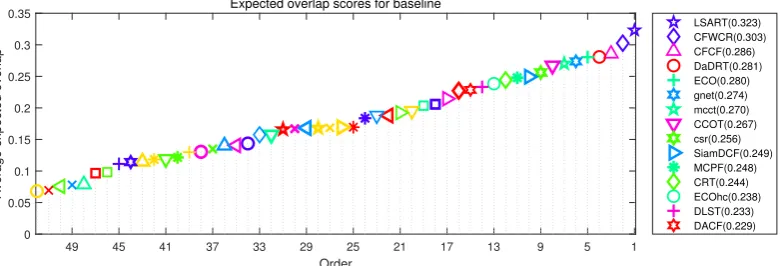
Figure9illustrates the EAO ranking. Our tracker achieves the remarkable rank (4th). VOT-2017 report [58] recommends a very strict state-of-the-art bound. Any tracker exceeding 0.201 under EAO metric on the VOT17 benchmark is considered the state-of-the-art. The performance of DaDRT is on par with the ECO and better than CCOT, MCPF and CRT. According to the definition of the VOT report, all these trackers are state-of-the-art.

1 5 9 13 17 21 25 29 33 37 41 45 49

Order 0

0.05 0.1 0.15 0.2 0.25 0.3 0.35

Average expected overlap

Expected overlap scores for baseline

[image:14.595.105.496.239.372.2]

LSART(0.323) CFWCR(0.303) CFCF(0.286) DaDRT(0.281) ECO(0.280) gnet(0.274) mcct(0.270) CCOT(0.267) csr(0.256) SiamDCF(0.249) MCPF(0.248) CRT(0.244) ECOhc(0.238) DLST(0.233) DACF(0.229)

Figure 9. Expected average overlap plot for VOT17 challenge with the proposed Distractor-aware Deep Regression Tracking (DaDRT) tracker. Only the top 15 performing trackers are labeled for clarity. Results are best viewed on high-resolution displays.

5.3. Ablation Studies

In DaDRT, we trained the regression network using three convolutional layers and distractor-aware loss. We conducted several experiments to validate the effectiveness of each component. By choosing two of the three used convolutional layers as features, we implemented three alternative approaches to validate multiple convolutional-layer connections. We denoted the three approaches as DaDRT_34, DaDRT_45, and DaDRT_35, where numbers indicate the used convolutional layers. Figure10shows the evaluation results on the OTB-15 dataset. We observe that only taking two convolutional layers as features could also achieve great performance compared with other state-of-the-art trackers. Furthermore, the combination across low- and high-level abstractions achieves better accuracy. The performance of DaDRT_34 and DaDRT_35 was almost the same, and the performance of DaDRT_45 was far behind. The evaluation results indicate that spatial detail is more important than semantic abstraction in learning regression networks.

(15)

0 5 10 15 20 25 30 35 40 45 50

Location error threshold 0 0.1 0.2 0.3 0.4 0.5 0.6 0.7 0.8 0.9 1 Precision

DaDRT [0.942] DaDRT_35 [0.930] DaDRT_34 [0.930] VITAL [0.918] PSCF [0.918] ECO [0.910] DSLT [0.907] C-COT [0.903] DAT [0.895] DaDRT_45 [0.894]

[image:15.595.79.520.86.271.2]

DaDRT [0.717] DaDRT_34 [0.708] DaDRT_35 [0.693] ECO [0.691] VITAL [0.682] PSCF [0.682] C-COT [0.673] DAT [0.668] DaDRT_45 [0.666] DSLT [0.658]

Figure 10.Ablation-study results on the OTB-15 dataset using one-pass evaluation. The numbers in the legend indicate the average distance-precision scores at 20 pixels and the area-under-curve success scores, respectively. Results are best viewed on high-resolution displays.

0 10 20 30

epoch 0 0.5 1 1.5 2 2.5 3 3.5 4 L2LossDA train

0 10 20 30

epoch 0 10 20 30 40 50 60 70 80 90 100 L2LossED train

0 10 20 30 epoch 1100 1200 1300 1400 1500 1600 1700 1800 1900 L2LossED train

0 10 20 30 epoch 0 0.2 0.4 0.6 0.8 1 1.2 1.4 L2LossHN train

0 10 20 30 epoch 1400 1500 1600 1700 1800 1900 2000 2100 2200 2300 L2LossED train

[image:15.595.89.512.321.414.2]

0 10 20 30 epoch 0 0.2 0.4 0.6 0.8 1 1.2 L2LossSK train

Figure 11. Training progress on different data-imbalance schemes. Each pair illustrates strategy loss and real Euclidean loss. With the same training conditions, all scheme losses rapidly converge. However, the HN and SK losses emerge with large displacement in ED loss. The training process actually requires more training epochs to prevent model overfitting. The proposed distractor-aware loss method can converge rapidly without overfitting. Results are best viewed on high-resolution displays.

5.4. Qualitative Evaluation

(16)

#0070 #0100 #0140 #0030 #0070 #0660

#0020 #0060 #0100 #0120 #0270 #0380

#0150 #0180 #0230 #0130 #0230 #0440

#0050 #0100 #0170 #0190 #0240 #0270

#0120 #0210 #0280 #0060 #0080 #0150

#0040 #0100 #0150 #0040 #0080 #0100

[image:16.595.72.522.86.374.2]

DaDRT CREST VITAL ECO DSLT HCF

Figure 12.Qualitative results comparing DaDRT with other trackers (ECO, VITAL, CREST, DSLT, HCF)

on 12 challenging sequences (from left to right and top to down:bike,basketball,bolt2,soccer,carscale,

clifbar,diving,freeman4,girl2,human3,motorrolling and matrix, respectively). The proposed DaDRT

tracker performed favorably against state-of-the-art methods. In the very challengingsoccer,clifbar, and

motorrollingsequences, DaDRT can always track to the target when most other trackers fail. Results are

best viewed on high-resolution displays.

5.5. Failure Case

We show some typical failure cases of the proposed tracker in Figure13. The proposed method failed in these cases mainly because of long-term occlusions or nonrigid deformation with scale change. The incremental frame-by-frame model update scheme may draft to the occlusions when long-term occlusions occur (e.g.,bird1). On the other hand, for nonrigid deformation with scale change (e.g.,jump,trans,ironman), the model must take a significant learning to account for large appearance changes. The proposed method balances this dilemma with an asuassive model update pace, which cannot take care of different challenges at the same time. Considering an effective discriminative strategy to distinguishthe different situations may help to alleviate this problem to some extent.

#0080 #0170 #0190 _#0010 _#0020 _#0050

#0040 #0060 #0100 #0010 #0110 #0150

[image:16.595.80.519.601.690.2]

(17)

6. Conclusions

In this paper, we proposed novel distractor-aware loss to alleviate the data-imbalance issue in learning regression networks. This enables the model to focus on positive and hard-negative samples during the training process. We also applied a hierarchy-normalized concatenation scheme to improve regression learning by exploiting strong representation across multiple convolutional layers. The proposed regression network is fully differentiable and can be trained end to end. Furthermore, incorporating other types of features is straightforward. Extensive experiments on five benchmarks demonstrate that the proposed DaDRT tracker performs favorably against state-of-the-art methods.

Author Contributions: conceptualization, M.D., Y.D., and X.M.; investigation, Y.D.; methodology, M.D. and Y.D.; project administration, Y.D. and X.M.; software, M.D.; supervision, Y.D., X.M., and H.-L.W.; validation, M.D.; visualization, M.D.; writing—original draft, M.D.; writing—review and editing, Y.D., H.-L.W., and Y.Z.

Funding:This research received no external funding.

Conflicts of Interest:The authors declare no conflict of interest. References

1. Wu, Y.; Lim, J.; Yang, M.H. Online object tracking: A benchmark. In Proceedings of the IEEE Conference on

Computer Vision and Pattern Recognition, Portland, OR, USA, 23–28 June 2013; pp. 2411–2418.

2. Wu, Y.; Lim, J.; Yang, M.H. Object tracking benchmark. IEEE Trans. Pattern Anal. Mach. Intell. 2015,

37, 1834–1848. [CrossRef] [PubMed]

3. Mueller, M.; Smith, N.; Ghanem, B. A benchmark and simulator for uav tracking. InEuropean Conference on

Computer Vision; Springer International Publishing: New York, NY, USA, 2016; pp. 445–461.

4. Possegger, H.; Mauthner, T.; Bischof, H. In defense of color-based model-free tracking. In Proceedings

of the IEEE Conference on Computer Vision and Pattern Recognition, Boston, MA, USA, 7–12 June 2015; pp. 2113–2120.

5. Kwon, J.; Lee, K.M. Tracking by sampling trackers. In Proceedings of the 2011 IEEE International Conference

on Computer Vision (ICCV), Barcelona, Spain, 6–13 November 2011; pp. 1195–1202.

6. Wang, D.; Lu, H.; Yang, M.H. Online object tracking with sparse prototypes.IEEE Trans. Image Process.2013,

22, 314–325. [CrossRef] [PubMed]

7. Wang, D.; Lu, H.; Xiao, Z.; Yang, M.H. Inverse sparse tracker with a locally weighted distance metric.

IEEE Trans. Image Process.2015,24, 2646–2657. [CrossRef] [PubMed]

8. Bao, C.; Wu, Y.; Ling, H.; Ji, H. Real time robust l1 tracker using accelerated proximal gradient approach.

In Proceedings of the 2012 IEEE Conference on Computer Vision and Pattern Recognition (CVPR), Providence, RI, USA, 16–21 June 2012; pp. 1830–1837.

9. Liu, B.; Huang, J.; Yang, L.; Kulikowsk, C. Robust tracking using local sparse appearance model and

k-selection. In Proceedings of the 2011 IEEE Conference on Computer Vision and Pattern Recognition (CVPR), Colorado Springs, CO, USA, 20–25 June 2011; pp. 1313–1320.

10. Zhang, T.; Liu, S.; Xu, C.; Yan, S.; Ghanem, B.; Ahuja, N.; Yang, M.H. Structural sparse tracking.

In Proceedings of the IEEE Conference on Computer Vision and Pattern Recognition, Boston, MA, USA, 7–12 June 2015; pp. 150–158.

11. Hare, S.; Golodetz, S.; Saffari, A.; Vineet, V.; Cheng, M.M.; Hicks, S.L.; Torr, P.H. Struck: Structured output

tracking with kernels.IEEE Trans. Pattern Anal. Mach. Intell.2016,38, 2096–2109. [CrossRef] [PubMed]

12. Wang, M.; Liu, Y.; Huang, Z. Large margin object tracking with circulant feature maps. In Proceedings of

the IEEE Conference on Computer Vision and Pattern Recognition, Honolulu, HI, USA, 21–26 July 2017; pp. 21–26.

13. Grabner, H.; Grabner, M.; Bischof, H. Real-time tracking via on-line boosting. Bmvc2006,1, 6.

14. Zhang, L.; Varadarajan, J.; Suganthan, P.N.; Ahuja, N.; Moulin, P. Robust visual tracking using oblique

random forests. In Proceedings of the IEEE Conference on Computer Vision and Pattern Recognition, Honolulu, HI, USA, 21–26 July 2017; pp. 5589–5598.

15. Babenko, B.; Yang, M.H.; Belongie, S. Robust object tracking with online multiple instance learning.

(18)

16. Henriques, J.F.; Caseiro, R.; Martins, P.; Batista, J. Exploiting the circulant structure of tracking-by-detection

with kernels. InEuropean Conference on Computer Vision; Springer: Berlin/Heidelberg, Germany, 2012;

pp. 702–715.

17. Henriques, J.F.; Caseiro, R.; Martins, P.; Batista, J. High-speed tracking with kernelized correlation filters.

IEEE Trans. Pattern Anal. Mach. Intell.2015,37, 583–596. [CrossRef] [PubMed]

18. Li, Y.; Zhu, J. A scale adaptive kernel correlation filter tracker with feature integration. InEuropean Conference

on Computer Vision; Springer International Publishing: New York, NY, USA, 2014; pp. 254–265.

19. Danelljan, M.; Häger, G.; Khan, F.S.; Felsberg, M. Discriminative scale space tracking. IEEE Trans. Pattern

Anal. Mach. Intell.2017,39, 1561–1575. [CrossRef]

20. Kiani Galoogahi, H.; Sim, T.; Lucey, S. Correlation filters with limited boundaries. In Proceedings of the IEEE

Conference on Computer Vision and Pattern Recognition, Boston, MA, USA, 7–12 June 2015; pp. 4630–4638.

21. Galoogahi, H.K.; Fagg, A.; Lucey, S. Learning Background-Aware Correlation Filters for Visual Tracking.

In Proceedings of the IEEE Conference on Computer Vision and Pattern Recognition, Honolulu, HI, USA, 21–26 July 2017; pp. 1144–1152.

22. Danelljan, M.; Hager, G.; Shahbaz Khan, F.; Felsberg, M. Learning spatially regularized correlation filters for

visual tracking. In Proceedings of the IEEE International Conference on Computer Vision, Boston, MA, USA, 7–12 June 2015; pp. 4310–4318.

23. Mueller, M.; Smith, N.; Ghanem, B. Context-aware correlation filter tracking. In Proceedings of the IEEE

Conference on Computer Vision and Pattern Recognition (CVPR), Honolulu, HI, USA, 21–26 July 2017; Volume 2, p. 6.

24. Ma, C.; Yang, X.; Zhang, C.; Yang, M.H. Long-term correlation tracking. In Proceedings of the IEEE

Conference on Computer Vision and Pattern Recognition, Boston, MA, USA, 7–12 June 2015; pp. 5388–5396.

25. Bertinetto, L.; Valmadre, J.; Golodetz, S.; Miksik, O.; Torr, P.H. Staple: Complementary learners for real-time

tracking. In Proceedings of the IEEE Conference on Computer Vision and Pattern Recognition, Las Vegas, NV, USA, 27–30 June 2016; pp. 1401–1409.

26. Girshick, R. Fast r-cnn. In Proceedings of the IEEE International Conference on Computer Vision, Santiago,

Chile, 7–13 December 2015; pp. 1440–1448.

27. Long, J.; Shelhamer, E.; Darrell, T. Fully convolutional networks for semantic segmentation. In Proceedings

of the IEEE Conference on Computer Vision and Pattern Recognition, Boston, MA, USA, 7–12 June 2015; pp. 3431–3440.

28. Simonyan, K.; Zisserman, A. Very deep convolutional networks for large-scale image recognition. arXiv

2014, arXiv:1409.1556.

29. Ma, C.; Huang, J.B.; Yang, X.; Yang, M.H. Hierarchical convolutional features for visual tracking.

In Proceedings of the IEEE International Conference on Computer Vision, Santiago, Chile, 7–13 December 2015; pp. 3074–3082.

30. Danelljan, M.; Hager, G.; Shahbaz Khan, F.; Felsberg, M. Convolutional features for correlation filter based

visual tracking. In Proceedings of the IEEE International Conference on Computer Vision Workshops, Santiago, Chile, 7–13 December 2015; pp. 58–66.

31. Danelljan, M.; Robinson, A.; Khan, F.S.; Felsberg, M. Beyond correlation filters: Learning continuous

convolution operators for visual tracking. InEuropean Conference on Computer Vision; Springer International

Publishing: New York, NY, USA, 2016; pp. 472–488.

32. Danelljan, M.; Bhat, G.; Khan, F.S.; Felsberg, M. ECO: Efficient Convolution Operators for Tracking.

In Proceedings of the IEEE Conference on Computer Vision and Pattern Recognition (CVPR), Honolulu, HI, USA, 21–26 July 2017; Volume 1, pp. 6638–6646.

33. Danelljan, M.; Bhat, G.; Gladh, S.; Khan, F.S.; Felsberg, M. Deep motion and appearance cues for visual

tracking. Pattern Recognit. Lett.2018. [CrossRef]

34. Wang, N.; Yeung, D.Y. Learning a Deep Compact Image Representation for Visual Tracking. In Proceedings

of the International Conference on Neural Information Processing Systems, Lake Tahoe, NV, USA, 5–10 December 2013; pp. 809–817.

35. Wang, L.; Ouyang, W.; Wang, X.; Lu, H. Visual tracking with fully convolutional networks. In Proceedings of

(19)

36. Nam, H.; Han, B. Learning multi-domain convolutional neural networks for visual tracking. In Proceedings of the IEEE Conference on Computer Vision and Pattern Recognition, Las Vegas, NV, USA, 27–30 June 2016; pp. 4293–4302.

37. Bertinetto, L.; Valmadre, J.; Henriques, J.F.; Vedaldi, A.; Torr, P.H. Fully-convolutional siamese networks for

object tracking. InEuropean Conference on Computer Vision; Springer International Publishing: New York, NY,

USA, 2016; pp. 850–865.

38. Song, Y.; Ma, C.; Gong, L.; Zhang, J.; Lau, R.W.; Yang, M.H. Crest: Convolutional residual learning for visual

tracking. In Proceedings of the IEEE Conference on Computer Vision and Pattern Recognition (CVPR), Honolulu, HI, USA, 21–26 July 2017; pp. 2574–2583.

39. Lu, X.; Ma, C.; Ni, B.; Yang, X.; Reid, I.; Yang, M.H. Deep regression tracking with shrinkage loss. InEuropean

Conference on Computer Vision; Springer International Publishing: New York, NY, USA, 2018; pp. 353–369.

40. Doulamis, N. Adaptable deep learning structures for object labeling/tracking under dynamic visual

environments.Multimed. Tools Appl.2017,77, 1–39. [CrossRef]

41. Chen, K.; Tao, W. Convolutional regression for visual tracking.IEEE Trans. Image Process.2018,27, 3611–3620.

[CrossRef] [PubMed]

42. Song, Y.; Ma, C.; Wu, X.; Gong, L.; Bao, L.; Zuo, W.; Shen, C.; Lau, R.; Yang, M.H. VITAL: VIsual Tracking via

Adversarial Learning.arXiv2018, arXiv:1804.04273.

43. Lin, T.Y.; Goyal, P.; Girshick, R.; He, K.; Dollár, P. Focal loss for dense object detection.IEEE Trans. Pattern

Anal. Mach. Intell.2018. . [CrossRef] [PubMed]

44. Yilmaz, A.; Javed, O.; Shah, M. Object tracking: A survey. ACM Comput. Surv. (CSUR)2006, 38, 13.

[CrossRef]

45. Smeulders, A.W.; Chu, D.M.; Cucchiara, R.; Calderara, S.; Dehghan, A.; Shah, M. Visual tracking:

An experimental survey.IEEE Trans. Pattern Anal. Mach. Intell.2014,36, 1442–1468. [PubMed]

46. Bolme, D.S.; Beveridge, J.R.; Draper, B.A.; Lui, Y.M. Visual object tracking using adaptive correlation

filters. In Proceedings of the 2010 IEEE Conference on Computer Vision and Pattern Recognition (CVPR), San Francisco, CA, USA, 13–18 June 2010; pp. 2544–2550.

47. Wang, C.; Zhang, L.; Xie, L.; Yuan, J. Kernel Cross-Correlator. In Proceedings of the AAAI Conference on

Artificial Intelligence (AAAI-18), New Orleans, LA, USA, 2–7 February 2018; pp. 4179–4186.

48. Danelljan, M.; Häger, G.; Khan, F.; Felsberg, M. Accurate scale estimation for robust visual tracking.

In Proceedings of the British Machine Vision Conference, Nottingham, UK, 1–5 September 2014; BMVA Press: Wales, UK, 2014.

49. Zhang, K.; Zhang, L.; Liu, Q.; Zhang, D.; Yang, M.H. Fast visual tracking via dense spatio-temporal context

learning. InEuropean Conference on Computer Vision; Springer International Publishing: New York, NY, USA,

2014; pp. 127–141.

50. Qi, Y.; Zhang, S.; Qin, L.; Yao, H.; Huang, Q.; Lim, J.; Yang, M.H. Hedged deep tracking. In Proceedings of

the IEEE Conference on Computer Vision and Pattern Recognition, Las Vegas, NV, USA, 27–30 June 2016; pp. 4303–4311.

51. Felzenszwalb, P.F.; Girshick, R.B.; McAllester, D. Cascade object detection with deformable part models.

In Proceedings of the 2010 IEEE Conference on Computer Vision and Pattern Recognition (CVPR), San Francisco, CA, USA, 13–18 June 2010; pp. 2241–2248.

52. Shrivastava, A.; Gupta, A.; Girshick, R. Training region-based object detectors with online hard example

mining. In Proceedings of the IEEE Conference on Computer Vision and Pattern Recognition, Las Vegas, NV, USA, 27–30 June 2016; pp. 761–769.

53. Maciejewski, T.; Stefanowski, J. Local neighbourhood extension of SMOTE for mining imbalanced data.

In Proceedings of the 2011 IEEE Symposium on Computational Intelligence and Data Mining (CIDM), Paris, France, 11–15 April 2011; pp. 104–111.

54. Huang, G.; Liu, Z.; Van Der Maaten, L.; Weinberger, K.Q. Densely connected convolutional networks.

In Proceedings of the IEEE Conference on Computer Vision and Pattern Recognition (CVPR), Honolulu, HI, USA, 21–26 July 2017; Volume 1, pp. 1–9.

55. Kukar, M.; Kononenko, I. Cost-Sensitive Learning with Neural Networks. In Proceedings of the 13th

European Conference on Artificial Intelligence (ECAI), Brighton, UK, 23–28 August 1998; pp. 445–449.

56. Khan, S.H.; Hayat, M.; Bennamoun, M.; Sohel, F.A.; Togneri, R. Cost-sensitive learning of deep feature

(20)

57. Liang, P.; Blasch, E.; Ling, H. Encoding color information for visual tracking: Algorithms and benchmark.

IEEE Trans. Image Process.2015,24, 5630–5644. [CrossRef]

58. Kristan, M.; Leonardis, A.; Matas, J.; Felsberg, M.; Pflugfelder, R.; Zajc, L.C.; Vojir, T.; Hager, G.; Lukezic, A.;

Eldesokey, A. The Visual Object Tracking VOT2017 Challenge Results. In Proceedings of the IEEE

International Conference on Computer Vision Workshop, Venice, Italy, 22–29 October 2017; pp. 1949–1972.

59. He, K.; Zhang, X.; Ren, S.; Sun, J. Delving deep into rectifiers: Surpassing human-level performance on

imagenet classification. In Proceedings of the IEEE International Conference on Computer Vision, Santiago, Chile, 7–13 December 2015; pp. 1026–1034.

60. Vedaldi, A.; Lenc, K. Matconvnet: Convolutional neural networks for matlab. In Proceedings of the 23rd

ACM International Conference on Multimedia (ACM), Brisbane, Australia, 26–30 October 2015; pp. 689–692.

61. Wang, Q.; Gao, J.; Xing, J.; Zhang, M.; Hu, W. Dcfnet: Discriminant correlation filters network for visual

tracking. arXiv2017, arXiv:1704.04057.

62. Ma, C.; Huang, J.B.; Yang, X.; Yang, M.H. Adaptive correlation filters with long-term and short-term memory

for object tracking. Int. J. Comput. Vis.2018,126, 771–796. [CrossRef]

63. Zhang, T.; Xu, C.; Yang, M.H. Multi-task correlation particle filter for robust object tracking. In Proceedings

of the IEEE Conference on Computer Vision and Pattern Recognition, Honolulu, HI, USA, 21–26 July 2017; Volume 1, pp. 4700–4708.

64. Danelljan, M.; Hager, G.; Shahbaz Khan, F.; Felsberg, M. Adaptive decontamination of the training set:

A unified formulation for discriminative visual tracking. In Proceedings of the IEEE Conference on Computer Vision and Pattern Recognition, Las Vegas, NV, USA, 27–30 June 2016; pp. 1430–1438.

65. Sui, Y.; Wang, G.; Zhang, L. Correlation filter learning toward peak strength for visual tracking.

IEEE Trans. Cybern.2018,48, 1290–1303. [CrossRef] [PubMed]

66. Hong, S.; You, T.; Kwak, S.; Han, B. Online tracking by learning discriminative saliency map with

convolutional neural network. In Proceedings of the International Conference on Machine Learning,

Lille, France, 6–11 July 2015; pp. 597–606.

67. Zhang, J.; Ma, S.; Sclaroff, S. MEEM: Robust tracking via multiple experts using entropy minimization.

InEuropean Conference on Computer Vision; Springer International Publishing: New York, NY, USA, 2014; pp.

188–203.

68. Hong, Z.; Chen, Z.; Wang, C.; Mei, X.; Prokhorov, D.; Tao, D. Multi-store tracker (muster): A cognitive

psychology inspired approach to object tracking. In Proceedings of the IEEE Conference on Computer Vision and Pattern Recognition, Boston, MA, USA, 7–12 June 2015; pp. 749–758.

69. Ma, C.; Huang, J.B.; Yang, X.; Yang, M.H. Robust visual tracking via hierarchical convolutional features.

IEEE Trans. Pattern Anal. Mach. Intell.2018. . [CrossRef] [PubMed]

70. Yun, S.; Choi, J.; Yoo, Y.; Yun, K.; Jin, Y.C. Action-Decision Networks for Visual Tracking with Deep

Reinforcement Learning. In Proceedings of the IEEE Conference on Computer Vision and Pattern

Recognition, Honolulu, HI, USA, 21–26 July 2017; pp. 1349–1358.

71. Wang, L.; Ouyang, W.; Wang, X.; Lu, H. Stct: Sequentially training convolutional networks for visual

tracking. In Proceedings of the IEEE Conference on Computer Vision and Pattern Recognition, Las Vegas, NV, USA, 27–30 June 2016; pp. 1373–1381.

72. Gao, J.; Ling, H.; Hu, W.; Xing, J. Transfer learning based visual tracking with gaussian processes regression.

InEuropean Conference on Computer Vision; Springer International Publishing: New York, NY, USA, 2014; pp.

188–203.

73. Pu, S.; Song, Y.; Ma, C.; Zhang, H.; Yang, M.H. Deep Attentive Tracking via Reciprocative Learning.

In Proceedings of the Advances in Neural Information Processing Systems 31: Annual Conference on Neural Information Processing Systems 2018, NeurIPS 2018, Montreal, QC, Canada, 3–8 December 2018; pp. 1933–1943.

74. Fan, H.; Ling, H. Parallel tracking and verifying: A framework for real-time and high accuracy visual

tracking. In Proceedings of the IEEE International Conference on Computer Vision Workshop, Venice, Italy, 22–29 October 2017.

75. Li, B.; Yan, J.; Wu, W.; Zhu, Z.; Hu, X. High Performance Visual Tracking with Siamese Region

(21)

76. Zhu, Z.; Wang, Q.; Li, B.; Wu, W.; Yan, J.; Hu, W. Distractor-Aware Siamese Networks for Visual Object

Tracking. InEuropean Conference on Computer Vision; Springer International Publishing: New York, NY, USA,

2018; pp. 103–119.

77. Ning, J.; Yang, J.; Jiang, S.; Zhang, L.; Yang, M.H. Object tracking via dual linear structured SVM and explicit

feature map. In Proceedings of the IEEE Conference on Computer Vision and Pattern Recognition, Las Vegas, NV, USA, 27–30 June 2016; pp. 4266–4274.

78. Cai, B.; Xu, X.; Xing, X.; Jia, K.; Miao, J.; Tao, D. BIT: Biologically Inspired Tracker. IEEE Trans. Image Process.

Publ. IEEE Signal Process. Soc.2016,25, 1327–1339. [CrossRef]

79. Choi, J.; Chang, H.J.; Yun, S.; Fischer, T.; Demiris, Y.; Choi, J.Y. Attentional Correlation Filter Network

for Adaptive Visual Tracking. In Proceedings of the IEEE Conference on Computer Vision and Pattern Recognition, Honolulu, HI, USA, 21–26 July 2017; Volume 2, p. 7.

80. Sui, Y.; Zhang, Z.; Wang, G.; Tang, Y.; Zhang, L. Real-time visual tracking: Promoting the robustness of

correlation filter learning. InEuropean Conference on Computer Vision; Springer International Publishing: New

York, NY, USA, 2016; pp. 662–678.

81. Kalal, Z.; Mikolajczyk, K.; Matas, J. Tracking-learning-detection.IEEE Trans. Pattern Anal. Mach. Intell.2012,

34, 1409. [CrossRef] [PubMed]

c

2019 by the authors. Licensee MDPI, Basel, Switzerland. This article is an open access