Development of deterministic collision-avoidance algorithms for routing automated guided vehicles

Rochester Institute of Technology

RIT Scholar Works

Theses Thesis/Dissertation Collections

9-1-2008

Development of deterministic collision-avoidance

algorithms for routing automated guided vehicles

Follow this and additional works at:http://scholarworks.rit.edu/theses

This Thesis is brought to you for free and open access by the Thesis/Dissertation Collections at RIT Scholar Works. It has been accepted for inclusion in Theses by an authorized administrator of RIT Scholar Works. For more information, please [email protected].

Recommended Citation

Rochester Institute of Technology

Development of Deterministic Collision-avoidance

Algorithms for Routing Automated Guided Vehicles

A Thesis

Submitted in partial fulfillment of the

requirements for the degree of

Master of Science in Industrial Engineering

in the

Department of Industrial & Systems Engineering

Kate Gleason College of Engineering

by

Arun S. Pai

M.S., Mechanical Engineering, Rochester Institute of Technology, 2002

DEPARTMENT OF INDUSTRIAL AND SYSTEMS ENGINEERING

KATE GLEASON COLLEGE OF ENGINEERING

ROCHESTER INSTITUTE OF TECHNOLOGY

ROCHESTER, NEW YORK

CERTIFICATE OF APPROVAL

M.S. DEGREE THESIS

The M.S. Degree Thesis of Arun S. Pai

has been examined and approved by the

thesis committee as satisfactory for the

thesis requirement for the

Master of Science degree

Approved by:

____________________________________ Dr. Michael E. Kuhl, Thesis Advisor

____________________________________ Dr. Moises Sudit, Thesis Advisor

Table of Contents

1 INTRODUCTION AND PROBLEM MOTIVATION... 1

1.1 INTRODUCTION... 1

1.2 DESCRIPTION OF AN AGVS ... 2

1.3 PROBLEM MOTIVATION... 5

1.4 OUTLINE OF THE THESIS WORK... 6

2 PROBLEM STATEMENT ... 7

3 LITERATURE REVIEW ... 10

3.1 AGV ROUTING BASED ON GUIDE PATH LAYOUT... 10

3.2 OPTIMIZATION METHODS FOR AGV CONFLICT RESOLUTION AND ROUTE PLANNING... 13

4 SCOPE AND METHODOLOGY ... 16

4.1 SCOPE... 16

4.2 SOLUTION APPROACH... 17

5 EXPERIMENTS AND RESULTS ... 36

5.1 RESULTS AND DISCUSSION... 36

5.2 PHASE II - HEURISTIC DEVELOPMENT – PRELIMINARY ANALYSIS... 41

5.3 PHASE III: DESIGN OF EXPERIMENTS FOR HEURISTIC COMPARISONS / SELECTION... 43

5.4 DISCUSSION OF SOFTWARE PROGRAM DEVELOPED FOR THE PROBLEM FORMULATION.... 59

6 CONCLUSIONS ... 60

BIBLIOGRAPHY ... 62

APPENDICES ... 64

A.1 APPENDIX 1: SECONDARY MOTIVATION FOR THE RESEARCH WORK - AGV MODELING USING ARENA – A CASE STUDY... 64

A.2 APPENDIX 2: POTENTIAL MODEL EXTENSION PROBLEMS FOR FUTURE WORK... 67

A.3 APPENDIX 3: EXPERIMENTAL STUDIES – RAW DATA & CALCULATIONS... 72

A.4 APPENDIX 4: SOFTWARE CODE FOR OPTIMAL PROBLEM FORMULATION... 111

A.5 APPENDIX 5: LIST OF FILES CONTAINED IN THE CD ... 127

Abstract:

A manufacturing job spends a small portion of its total flow time being processed on machines, and during the remaining time, either it is in a queue or being transported from one work center to another. In a fully automated material-handling environment, automated guided vehicles (AGV) perform the function of transporting the jobs between workstations, and high operational costs are involved in these material-handling activities. Consequently, the AGV route schedule dictates subsequent work-center scheduling.

For an AGV job transportation schedule to be effective, the issue of collisions amongst AGV during travel needs to be addressed. Such collisions cause stalemate situations that potentially disrupt the flow of materials in the job shop, adding to the non-value time of job processing, and thus, increase the material handling and inventory holding costs. The current research goal was to develop a methodology that could effectively and efficiently derive optimal AGV routes for a given set of transportation requests, considering the issue of collisions amongst AGV during travel.

1 Introduction and Problem Motivation

1.1 Introduction

Material handling is an important aspect of any production system. Material handling

systems have been prevalent since the beginning of mass production, either as manual systems,

mechanical systems (forklifts, conveyors), or in more recent years as fully automated systems

(Automated Guided Vehicle Systems [AGVS] or Automatic Storage & Retrieval Systems

[AS/RS]). Due to the high operational costs attributed to material handling activities, for years

organizations have been looking for ways to minimize the time spent on material handling, and for

ways to optimize material handling operations. With technological advancements in use of

automated equipment such as conveyors and automated guided vehicles (AGV), companies now

have improved material handling alternatives. Particularly, due to the routing flexibility associated

with AGVs, their applications have spanned from use in distribution centers, warehouses, and

terminals to large-scale manufacturing in assembly facilities.

The following sections in the chapter present an overview of an AGV system, discuss the

advantages of using such a system, outline the important decision variables in an AGVS design,

and finally detail the motivation for pursuing this research work.

1.2 Description of an AGVS

An AGVS is an advanced material-handling system that involves one or more driverless

vehicles, each following a physical or virtual guide path under the control of a computer. Two

primary control systems are in use today. In the first type, the control lies in a simple central

computer inside the vehicle itself. In the second type of control, the vehicles have minimal

intelligence and an off-board computer controls the vehicles. The different components of an

AGVS include:

• The vehicle that consists of the frame, batteries, on-board charging unit, electrical system,

drive unit, steering, safety system, communication unit and the work platform;

• The guide path and guidance systems; and

• The floor and system controls.

1.2.1 Advantages of an AGVS

The advantages of an AGVS include reliability, automatic operation, flexibility in adapting

to changes in material flow, reduced labor and increased productivity, and automated interfaces

with other systems. Unlike conveyors or other material handling systems, AGV are small in size

and only move along the aisles. Hence, an AGVS offers additional benefits of reduced space

requirements. The real-time control of material handling that the AGVS offers helps in

identification of the parts, the routes they travel and the vehicles they travel in, resulting in a lower

WIP inventory, reduced tardiness, lower inventory costs and better response to demands

(Hammond, 1986). Thus, an AGVS can improve the working environment, reduces product

damage, and provides better inventory control and quality.

1.2.2 Critical Variables in an AGVS design

The system performance of an AGVS directly affects the performance of the whole facility.

To realize an AGVS full potential for flexibility, careful planning and control of the system design

and operation is essential. The enormity in design and hardware requirements of an AGVS

necessitates a number of variables to be considered at each level of the decision-making process.

The relevant issues can be divided into the following main categories: guide-path design,

estimating the required number of vehicles, vehicle scheduling, idle-vehicle positioning, battery

management, vehicle routing, and conflict resolution. These issues relate to different levels of the

decision-making process.

The guide-path design problem can be seen as a problem at the strategic level. The

decision at this stage has a strong effect on decisions at other levels. Issues at the tactical level

include estimating the number of vehicles, scheduling vehicle, positioning idle vehicles, and

managing battery-charging scheme. Finally, the vehicle routing and conflict resolution problems

are addressed at the operational level. During the design, implementation, and control of an

AGVS, interactions and iterations between the different decision levels should be accounted for.

An overview of these decision levels is outlined in Table 1.

Table 1: Important Decision-Variables in an AGVS Design

No. Decision level Type of decisions

1 Process focus Type and number of vehicles to be present in a system.

2 Equipment

considerations

Type of vehicle steering control, routing method, traffic management, load transfer mechanisms at load and unload points;

and monitoring of the AGVS.

3 Facility

considerations

Optimal number of workstations, optimal number of machines per workstation, optimal number of buffers; and optimal number of kits.

4 Workstation

considerations

Workstation layout; and even distribution of processing time over all the stations in the system.

5 Task-related

considerations

Transportation times based on considerations of number of job types, lot size descriptions and intensity of flow collisions.

6 Travel-related

considerations

Type of flow path, track layout, zoning considerations, dedication of the AGV, staging areas, load and unload times; and travel speeds of

the AGVs.

7 Schedule-related

considerations

Job dispatching rules, sequencing of moves requests, and intersection problems.

1.3 Problem Motivation

The motivation for this work is derived from insight into two separate yet similar

considerations – the primary motivation is the lack of a comprehensive methodology for

collision prevention and optimality in an AGV system, while the secondary motivation is glitch

in handling AGV deadlock situations in a commercial simulation software (ARENA) used for

modeling of AGV systems. The motivations are discussed in detail in the following sections.

1.3.1 Primary Motivation: Methodology for Collision Prevention and Optimality

Of all the decision variables summarized in Table 1, operational issues related to vehicle

travel and scheduling have been the major focus areas of research in recent times. This is

because of the mathematical complexities involved in their optimization.

AGV routing decisions are iteratively dependant on effective flow path designs. So,

AGV flow path decision considerations have been the major focus of investigations. As the

AGV travel layouts improved, focus shifted towards developing vehicle routing algorithms that

could conclusively address the issue of prevention of collisions amongst AGV during travel, and

effectively generating optimal vehicle routes relative to minimizing transportation time. The

rule-based strategies that have been developed since are not able to provide near-global optimal

solutions in computationally efficient times. Moreover, these techniques can be applied

effectively only to small-scale problem domains. Therefore, there is room for improvement in

AGV routing methodologies that include vehicle collision prevention, thus, stimulating the need

for a comprehensive and complete model for solving the problem. This is the primary

motivation for this study.

1.3.2 Secondary Motivation: Commercial Simulation Software for Modeling of AGV systems

Current commercial (off the shelf) simulation software such as ARENA can model

material handling systems. There is however a glitch in using such packages for AGV routing.

Although ARENA uses a collision detection strategy in such situations, studies indicate that if

proper control is not specified for the transporter, the software terminates on detection of a

collision or deadlock situation amongst vehicles. To illustrate this, a case study is discussed in

the following sub-section.

The results of the study (outlined in Appendix A.1) were a secondary motivation for the

author to conduct research in AGV routing. It is hoped that from this work an optimal AGV

routing methodology with collision prevention can be developed, that could be integrated with

simulation systems such as ARENA in future research.

1.4 Outline of the Thesis Work

This thesis document is organized as follows: Chapter 2 contains the Problem Statement.

Chapter 3 is a thorough review of the relevant literature. Chapter 4 discusses the scope of work

and the approach used to solve the problem (model formulation and the design of the different

heuristics). Chapter 5 summarizes the results inclusive of optimality runs, experimental designs

and statistical analysis. The conclusions of the research work are presented in Chapter 6.

2 Problem

Statement

A manufacturing job can spend on an average only 5% of its total flow time being

processed on machines, and during the remaining time, either it is in a queue or being transported

from one work center to another (Han et al., 1989). In a fully automated material-handling

environment, AGVs perform the function of transporting the jobs between workstations, and

high operational costs are involved in these material-handling activities. AGV scheduling

influences subsequent work-center scheduling, and dictates the overall production schedule.

Therefore, there is a potential loss of overall system performance, and an increase in the material

handling and inventory holding costs, if the AGV routing is not effective.

In an AGV routing system based on a deterministic approach, all tasks are known prior to

the planning period. The complete AGV routes can be developed before vehicles carry them out.

Such a problem is similar to the pick-up and delivery problem with time windows (PDPTW),

which often has travel time minimization or minimization of the number of vehicles as

objectives. The PDPTW problem is known to be NP-hard (Dumas et al., 1991), so it is

infeasible to develop an algorithm to solve this type of problem in polynomial time. Due to this

reason, heuristics are the most appropriate approach to cope with this type of problem. Past

researches like Gaskins et al. (1987); Savelsbergh et al. (1995); Seo et al. (1995); Bilge et al.

(1995) and Ulusoy et al. (1997) have focused on developing approaches that identify imminent

collisions through forward sensing and their aversion through vehicle backtracking or rerouting.

In summary, current approaches are based on forward sensing instead of a collision

prevention scheme. They employ the concept of shortest travel distance, thereby arriving at

schedules that are likely far away from an optimal route. A better approach that can predict near

optimal routes should include constraints that totally prevent AGV collisions in the route

scheduling model. Collisions cause stalemate situations that potentially disrupt the flow of

materials in the job shop, adding to the non-value time of job processing, and thus, increase the

material handling and inventory holding costs.

Hence, the research goal is to develop a methodology that can derive optimal AGV routes

for a given set of transportation requests, considering the issue of collisions amongst AGV

during travel. Secondly, computationally the program should solve problems in “practical

feasible time” (based on application). Developing a methodology that can effectively and

efficiently address these issues is the overall goal of this work.

The problem statement can be summarized as developing a route planning system that:

• Works effectively for any type of AGV guide path layout;

• Can optimally derive vehicle routes for a deterministic set of transportation requests;

• Accounts for collision avoidance amongst vehicles during travel; and,

• Arrives at solutions in a practically feasible (based on application) computation time.

As part of the solution approach in the proposed work, an integer linear program is

formulated in Phase I with the capability of optimally predicting the AGV routes for a

deterministic set of transportation requests. Collision avoidance constraints are developed in this

model. The model is programmed using Visual Basic / CPLEX 9.0 / OPL 3.7, and the program

feasibility is experimentally analyzed for different problem domain specifications. Due to the

complexity and combinatorial nature of the formulation in Phase I, computationally the

mathematical model is expected to be NP-Hard. Hence, to improve the efficiency of the

computation, in Phase II, heuristics are developed to relax the computational complexity of the

original problem. In Phase III, experimental techniques are used to compute the lower and upper

bounds of the original problem. The performances of the different heuristics are compared using

experimental analysis.

3 Literature

Review

This chapter presents a review of available AGV literature in the areas of vehicle dispatching,

vehicle routing and traffic control.

3.1 AGV Routing Based on Guide Path Layout

The following sub-sections detail the available literature for the different types of guide

paths used in AGV systems.

3.1.1 Uni-Directional Guide Path

The earliest research on AGVS modeling in a warehouse / manufacturing set-up

addressed process and travel-related issues such as vehicle fleet sizing and uni-directional guide

path layout. The primary focus was to maximize space utilization, and since in such a set-up,

most of the floor space is taken by the storage facility, the AGV flow paths were restricted to a

series of narrow aisles, and hence, it was mathematically and computationally infeasible to

model a bi-directional multi-AGV routing layout. The seminal paper in this area was by

Maxwell et al. (1982). This work computed the minimum number of AGVs required in a

time-independent environment to efficiently transfer material from one facility to another. However,

since time was essentially ignored, the authors assumed no congestion or blocking in the system.

This paper led to many extensions and research in related issues and is cited extensively.

Gaskins et al. (1987); Hodgson et al. (1987); Kaspi et al. (1990); and Goetz et al. (1990)

incorporated the time element in the AGVS modeling to determine the directional flow on a

uni-directional AGV path. The objective of these studies was to minimize the total distance traveled,

given a known set of requests between pair of locations. The assumptions made in these studies,

however, restricted the robustness of the models. Gaskins et al. (1987) only considered the

movement of loaded vehicles and assumed that the flow path movement of the AGV was

restricted to certain areas such as aisles. The model could not be generalized to include factors

such as the travel of the unloaded vehicles, vehicle blocking and congestion. Similarly, Hodgson

et al. (1987) used Markov decision processes to develop AGVS dispatching rules in a

time-dependent environment. Such a procedure was however, increasingly difficult to model even for

a simple AGVS due to the large number of states involved. This further necessitated several

constraints to be set in for the semi-Markov problem to be tractable. Kaspi et al. (1990) solved

the optimal flow path design problem in a uni-directional network using a branch and bound

technique, while Goetz et al. (1990) developed an algorithm to minimize the total AGV travel

distance in a uni-directional layout. It was observed that for larger problem sizes, both of the

above models were difficult to solve.

Due to computational and mathematical complexities involved in the routing algorithms,

in the mid-nineties; focus shifted towards iterative, phased approaches in algorithm development.

Seo et al. (1995) were the initial researchers to design a two-stage method to solve the routing

problem; wherein the first stage uses a binary integer program and considers the AGV loaded

travel in its objective. The second stage takes into account the empty travel of the AGV, and is

used only if an optimal closed solution is not obtained in the first stage. A branch and bound

heuristic was used to solve the problem. The process was found effective to solve a problem

with nine workstations. The method was computationally efficient, however, its efficiency in

case of larger real world problems were not examined. Moreover, the model was not robust

enough to be effectively scaled-up for bi-directional networks.

It was evident from the results of the above studies that even the most efficient

uni-directional system would increase the travel times between some pair of locations. Hence, the

very objective to minimize the total travel time for the AGV in a collision –free environment

would not be accomplished. This necessitated a need to research the possible advantages and

complications in a bi-directional flow path.

3.1.2 Bi-Directional Guide Path

The earliest research on bi-directional AGVS modeling by Egbelu et al (1986) discussed

the different types of bi-directional travel guide paths. The study was based on an assumption

that all flow within an aisle can be in either direction; however, at any moment in time all flow

within a single aisle is in the same direction. The results of the simulation study conducted by

the authors demonstrated that a bi-directional system required fewer vehicles to achieve the same

workload as compared to a uni-directional system over the same layout. Similarly, Zeng et al.

(1991) investigated a less restrictive bi-directional option, in which vehicles were allowed to

travel along the same aisle in opposite directions, as long as a collision situation is not detected.

Their solution introduced a time element, and was based on an extension of the petri-net

approach. However, their algorithm could not suggest an alternative route in cases where a

collision is detected. So, the mid-nineties saw a shift in research focus towards collision

detection. Krishnamurthy et al. (1993) used a column generation collision detection technique to

develop a conflict free routing algorithm for AGV. They considered a bi-directional network

and sub-divided the problem into a master problem and a sub problem. The authors attempted

several empirical solution techniques to solve the sub problem and the link between the sub and

the master problems. With technological advancements, AGV collision avoidance rather than

collision detection became research goals for a comprehensive optimal routing system.

Dowsland et al. (1994) were the initial researchers to focus on this concept. They formulated the

AGV flow path as a graph network and considered the different cases where collision might

occur at a given node. They used delays and deviations along the spur of a node to determine the

collision avoidance. The authors, however, recommended a need for future study into further

validations of their results using a more comprehensive set of simulations. In the late nineties,

Endo et al. (1998) proposed a petri-net approach to solve the motion-planning problem for

multiple AGV. In a separate work, Endo et al. (2000) developed a genetic algorithm to tackle

the collision avoidance problem. However, both these methods were applicable only to the small

sized problems.

3.2 Optimization Methods for AGV Conflict resolution and Route Planning

It is difficult to manage an AGV system efficiently, and it is an issue in itself. This issue

includes several sub issues such as AGV scheduling, idle vehicle positioning, vehicle routing and

conflict resolution. In actuality, online scheduling and dispatching systems are much more

popular than offline scheduling due to the stochastic nature of AGV systems, and perform better

than simple dispatching systems (Yang et al., 1999). However, there is no secret that modeling

them is much more complex and computationally cumbersome. In an offline (Pre-Planned)

scheduling system, all tasks are known prior to the planning period. The complete AGV routes

can be developed before vehicles carry them out. Past researches in this area like Gaskins et al.

(1987); Savelsbergh et al. (1995); Seo et al. (1995); Bilge et al. (1995) and Ulusoy et al. (1997)

have focused on developing approaches that identify imminent collisions through forward

sensing and their aversion through vehicle backtracking or rerouting. In summary, current

approaches are based on forward sensing instead of a collision prevention scheme. They employ

the concept of shortest travel distance, thereby arriving at schedules that are necessarily far away

from an optimal route. A better approach that can predict near optimal routes should include

constraints totally prevent AGV collisions in the route scheduling model.

Currently, conflict-free routing in AGV systems is established by means of one of the

following three approaches: (i) the problem elimination through the adoption of a segmented

path flow or tandem queue configuration (Egbelu et al., 1986); (ii) the identification of imminent

collisions through forward sensing and their aversion through vehicle backtracking and/or

rerouting (Zeng et al., 1991) and (Hsieh et al, 1998); or (iii) the imposition of zone control and

extensive route pre-planning, typically based on deterministic timing of the vehicle traveling and

docking stages (Ho, 2000). Among these three approaches, the segmented path flow-based

approach presents the highest robustness to the system randomness, but at the cost of restricted

vehicle routings and the need for complicated handling operations. These conflict-free routing

systems make use of dispatching rules for initial vehicle assignment. Egbelu et al. (1984) were

the first researchers to characterize dispatching rules for AGV using simulation. They

considered two categories of rules (the work center initiated and the vehicle initiated) for vehicle

dispatching decisions. The rules for the work center initiated tasks included nearest vehicle

(NV), farthest vehicle (FV) and least utilized vehicle (LUV). For vehicle initiated tasks, the

rules included modified first come first serve (MFCFS), shortest travel time/distance, longest

travel time/ distance and maximum outgoing queue size (MOQS). However, their study focused

more on dispatching rules in a unidirectional network.

Kim et al. (1993) used the concept of time windows to analyze the problem of routing a

single AGV from source to destination in the shortest time duration. They maintained a table of

scheduled arrival and departure times for all other AGV for each node. The authors then defined

a time window to be the duration between the entry and exit at a node, such that each time

window was uniquely reserved for a vehicle with no other AGV allowed to cross that node

during this time period. At around the same time, Seifert et al. (1995) evaluated AGV routing

strategies using hierarchical simulation. Beyond the static deterministic approach that simply

follows the shortest travel distance, the authors also introduced a dynamic vehicle routing

strategy based on hierarchical simulation. They developed a generic concept in which the

current status of the system was used to embed sub simulations at each decision epoch to mimic

the future operation of the system. One of the major recommendations from the study was to

generate a sufficient number of alternative vehicle paths so that the critical bottlenecks could be

bypassed dynamically. Ho (2000) introduced the concept of a “dynamic-zone strategy” to

prevent vehicle collision. This strategy allows reassignment of a vehicle to a zone at any point of

time, and uses a zone adjustment procedure to change the area of a zone according to a current

production demand. A zone assistance procedure enables the vehicles to balance their workload

amongst each other at all instances of time. The strategy developed by Ho was based on the

assumption that the AGV system has a single-loop guide path. In addition, it is assumed that an

AGV can transport only one load at a time. In the present work, these issues have been

addressed conclusively.

4 Scope and Methodology

The following sections in this chapter detail the research scope, describe the mathematical

models formulated to solve the problem, and discuss the various heuristic algorithm approaches

developed to obtain computationally practical feasible solutions.

4.1 Scope

This research work focuses on optimization of routing AGVs based on prevention of

collision amongst the vehicles.

The research goal is to develop an optimally feasible and computationally practical AGV

routing system. The objective of the work is to determine an optimal transportation route and

timing for the different AGVs in the system, for any given “deterministic” set of transportation

requests.

The research vision is to develop a strong mathematical background (in the current work)

that could be used in the future to expand the proposed methodology in development of

optimally feasible solutions for a “dynamic” set of transportation requests. However, these

expanded studies are beyond the scope of the current work.

The research scope can be summarized as:

• Comprehensive mathematical representation of the variables in an AGV routing system,

independent of vehicle guide path layout;

• Incorporation of distinctive collision prevention constraints in the model;

• Formulation and programming of different heuristic procedures for problem solution in

practically feasible time;

• Selection of the best heuristic or combination of heuristics that could be used across

different AGV routing systems; and

• Dynamic simulation of the vehicle routes is out-of-scope of this work.

4.2 Solution Approach

The mathematical model is designed to incorporate the following routing elements:

• Allow AGVs to move on multiple paths yet have the ability to select the best path; and

• Allow the AGVs to move on paths with intersections, yet avoid collisions in a way that

best meets the needs of the facility.

The development of the solution methodology involves four (4) phases:

Phase I: Formulation of The Mathematical Model

In this phase, different solution formulation models are developed, progressively reiterated

and evaluated in terms of comprehensively capturing the problem domain and research

objectives. Based on the evaluation, an integer linear program (IP) is developed and selected

with the capability of optimally predicting the AGV routes for a deterministic set of

transportation requests. The model is based on inclusion of positioning constraints, motion

feasibility constraints, collision prevention constraints, target constraints, and integrality

constraints; that are developed to cover all aspects of AGV routing. The model is programmed

using OPL 3.7 and C++, while CPLEX 9.0 is used as the solver. Numerical examples are

presented in this phase to support model justification.

Phase II: Heuristic Development

Due to the complexity and combinatorial nature of the formulation in Phase I,

computationally it is NP-Hard. Hence, to improve the efficiency of the computation, in Phase II,

heuristic algorithms are developed that relax the computational complexity of the original

problem. In this phase, different heuristic procedures are designed, programmed and tested to

compute the upper bounds of the original formulation.

Phase III: Heuristic Selection

Experimental designs for different sized systems are conducted in this phase in order to

compare the performance of the different heuristics. For small-sized systems, the heuristic

results are compared to optimal solutions; while for large-sized systems, the bounds obtained

from different heuristic procedures are compared. Statistical techniques are used in the analysis.

The goal of this phase is to arrive at a robust heuristic / combination of heuristic procedures that

can be used across any sized routing system.

Phase IV: Conclusions and Scope for Future Work

The results from this work are summarized in this phase with segmented recommendations

for solution expansion to dynamic transportation request problem.

The conclusions and results drawn from each phase are progressively used to contribute to

the goal of subsequent phases, and to the overall research objectives.

4.2.1 Phase I: Formulation of The Mathematical Model

The AGV route-planning problem is defined as follows: A grid layout represents the

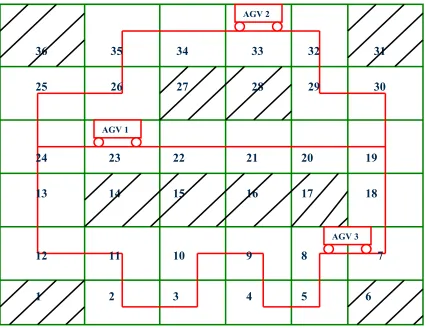
shop floor / distribution / warehouse center. Figure 1 shows a sample grid layout, with the

pre-designed AGV guide path represented by the red line.

1 2 3 4 5 6

12 11 10 9 8 7

13 14 15 16 17 18

24 23 22 21 20 19

25 26 27 28 29 30

36 35 34 33 32 31

AGV 1

AGV 2

AGV 3

Grid layout

Storage area

AGV path

Figure 1: Example of an AGV Grid Layout

In the sample grid layout presented in Figure 1, there are 36 grids in all. The grids that

are shaded represent the storage areas, and as such, the AGVs are not programmed to move into

these locations. The guide path is shown by the red solid line, and is indicative of a feasible

point for an AGV from any particular grid. For example, as shown in Figure 1, AGV 1 is located

at Grid 23 at initial time instant 0. At time instant 1, the program constraints the motion of AGV

1 to either Grid 24 or 22 or to stay at Grid 23 itself. There are pre-defined target grids which

have pre-defined destination nodes. The AGVs have capacities to carry load. For the

mathematical model, it is assumed that each AGV can at any time carry at most one load.

4.2.1.1 Model Assumptions

The following are the assumptions made in the formulation:

1. All the grids are rectangular in shape, and equal in dimensions.

2. All the AGV’s considered are capable of bi-directional travel.

3. The velocity for each AGV is constant, with the transportation time proportional to the

grid dimensions.

4. Every AGV has the same ability of transportation and carrying capacity.

5. Every AGV carries / delivers only one unit load at a time.

4.2.1.2 Nomenclature

The variables (other than the decision variables) that define the problem domain are

presented in this section. Section 4.2.1.3 discusses the decision variables used in the

formulation.

J = Number of AGVs in the system

T = Total time required to complete all deliveries in the system

I = Number of grid elements in the system grid

Fi = Set of feasible moves from grid i

H = Set of targets

ri = Destination node for the target at node i such that i∈H

4.2.1.3 Decision variables

Three (3) decision variables are used to completely define the problem. All the

capture the presence of an AGV j at a grid i at any particular time t; Y define the instance t

when a target i ∈ H is picked up by an AGV j; and are activated when the target i ∈ H is

delivered by the AGV j to the destination. These decision variables are further explained below.

ijt X

ijt

ijt Z

ijt X =

otherwise at time grid visits AGV an if 0

1 j i t

 

 for ∀i, ∀j, ∀t

ijt Y =

otherwise at time grid at target the up picks AGV an if 0

1 j i t

 

 for i∈H, ∀j, ∀t

ijt Z =

otherwise t at time n destinatio the to dropped is grid at target the if 0 1 i  

 for i∈H, ∀j, ∀t

4.2.1.4 Objective Function

The objective of the formulation is to minimize the total transportation time required for

target delivery. The mathematical model can be represented as:

Minimize w

Subject to all the constraints detailed in Section 4.2.1.5 Table 2. w is constrained by Equation 11 in Section 4.2.1.5 Table 2.

4.2.1.5 Mathematical Model – Constraints

The AGV routing path is developed with the objective that there are no vehicle

collisions at any point of time, each AGV maintains motion feasibility, and the whole process

minimizes the load transportation time in the application set-up. The model constraints detailed

in Table 2 incorporate each of these aspects, and can be broadly categorized as:

• AGV Positioning Constraints: Equation 1 defines the position of an AGV at any particular instance of time, while Equation 5 constraints an AGV to be present at a grid

where it picks up the target at that instance of time. Similarly, Equation 9 synchronizes

target deliverance to the requirement of AGV presence at the delivery point, at that

particular time.

• AGV Motion Feasibility Constraint: Equation 3 constraints subsequent AGV moves based on the feasibility moves on the guide path from any particular grid. In this

constraint, the model extends feasibility of moves for applicability in any type of AGV

guide path layout.

• Collision Prevention Constraints: Equations 2 and 10 are the collision prevention constraints that are responsible for the uniqueness of the model.

• Target Constraints: Equations 4, 6, 7 (or equivalently a combination of 7A and 7B) and 8 define the requirements of pick-up and delivery of targets.

• Integer Constraints: Equations 12 to 14 are binary constraints for the X’s, Y’s and Z’s.

The following section discusses in detail each of these constraints.

Table 2: Constraints in the Mathematical Model

Equation Description Equation _No.

∑

= I i

ijt X

1 for ∀j, ∀t

Any time an AGV will occupy

only one grid (1)

∑

≤ 1

for ∀i, ∀t Any time a grid would be occupied by a maximum of one AGV (2)

∑

- X_ijt ≥ 0

for ∀i, ∀j, ∀t

Continuity & feasibility (i.e.) For each successive time instance, an AGV should either stay at grid i or move to the next feasible grid

(3)

∑∑

for i∈H A target is picked by exactly _{one AGV (all time)} (4)

ijt

Y ≤ X_ijt for i∈H, ∀j,

∀t

An AGV picking up a load at grid I at time t must be located at grid I at time t

(5)

∑∑

for i∈H

A target that has been picked from grid i would be

delivered to the destination exactly once (6)

∑

>

∑

= T t

ijt tY

1 for i∈H, ∀j

The time at which the target is delivered to the destination exceeds the time when the target is picked up

(7)

Table 2 (continued): Constraints in the Mathematical Model

Constraint 7 can also be modeled as a combination of Constraints 7A and 7B:

∑

> Y_ijt for i∈H, ∀j,

∀t

The time at which the target is delivered to the destination exceeds the time when the target is picked up

(7A)

ijT

Y = 0

for i∈H, ∀j (7B)

∑∑

∈H = i t k ijk Z 1

+ C_j ≥

∑∑

∈H = i

t k

ijk

Y

1 for ∀j, ∀t

At any time, all the AGV’s should have picked total number of loads ≤ their capacities

(8)

ijt

Z ≤ _rjt

i

X for i∈H, ∀j,

∀t

The target is delivered only when the loaded AGV is at the destination

(9)

kjt

X + X_ilt + X_ijt+1 + X_klt+1 ≤ 3

for ∀i, ∀j, ∀t

and k∈

and l i F ∈J such that l≠j

If two AGV’s occupy adjacent grids at any time instant, they cannot switch their positions in the next time instant

(10)

w≥

∑∑

1 1 for i∈H

Constraint to minimize the total transportation time required for target delivery

(11)

ijt

X = 0 or 1 _{for ∀i, ∀j, ∀t Integer constraints} (12)

ijt

Y = 0 or 1 for i∈H, ∀j,

∀t Integer constraints (13)

ijt

Z = 0 or 1 for i∈H, ∀j,

∀t Integer constraints (14)

4.2.1.6 Solving Approach

The mathematical formulation was programmed using Optimization Programming

Language (OPL), and tested to provide an initial gauge of the computational capacity (solving

time) and computational accuracy (confirmation that all essential collision-prevention constraints

had been captured). It was found that for systems up to 5*5 grid layouts, the model provides an

optimal solution in a reasonable amount of time. However, for systems beyond a 25-grid layout,

the problem becomes NP-hard and development of heuristic algorithm(s) becomes essential

(described in following sections).

4.2.2 Phase II: Heuristic Development

A problem is assigned to the NP (nondeterministic polynomial time) class if it is

verifiable in polynomial time by a nondeterministic turing machine. A problem is said to be

NP-hard if an algorithm for solving it can be translated into one for solving any other NP-problem.

Due to the complexity and combinatorial nature of the mathematical formulation in Phase I,

computationally it was found to be NP-Hard. Hence, to improve the efficiency of the

computation, in Phase II, a heuristic solution of the formulation was mathematically required.

The heuristics functions can be divided into two groups of admissible and non-admissible

heuristics. An admissible heuristic is one that never overestimates the optimal cost, i.e. a lower

bound. In this work, since the IP is a minimization problem, the non-admissible heuristic would

provide an upper bound to the original problem. All the heuristics are computed by solving

deterministic relaxations of the original formulation.

The heuristic methods proposed in this work are developed using the dispatching

strategies characterized by Egbelu et al. (1984) as a basis. In this work, Egbelu’s rules have been

modified to account for specific characteristics of the problem under consideration. The

proposed heuristic methodology for the AGV routing is divided into two portions:

1. Development of heuristic priority rules to construct a flexible routing mechanism; and

2. Implementation of the routing system in a flexible software structure.

Multiple heuristics were proposed in initial feasibility studies, however, based on screening trials

on computational accuracy (comparison to optimal solution for small-sized systems), the

following 4 heuristic approaches were selected for subsequent experimental study purposes:

• The Greedy Approach;

• The Nearest Neighbor Approach;

• The Least Utilized AGV Approach; and

• The Modified Greedy Approach

The mathematical logic for each of the above heuristics is detailed in the following sections.

4.2.2.1 The Greedy Approach (G)

In order to reduce the computational time taken to solve the original formulation, the model

is solved in “h” iterations, where h equals the number of targets. This reduces the complexity of

the problem solved at each iteration. Each iteration involves solving a modified version of the

original problem, where only one target-AGV combination is selected by the OPL program such

that the selected target is delivered the earliest amongst all targets. The general steps in the

Greedy Approach are described below:

Step 1: For a set of j AGV and h targets, the OPL program decides the initial assignment of an AGV to a target with the earliest possible delivery time.

Step 2: In the next iteration, the locations of the AGV from Step 1 solution are fixed for

the time instances till the target is delivered. The program is solved to arrive at

the next AGV-target combination.

Step 3: Steps 1 and 2 are repeated for the remaining targets, and the program stopped when all the targets have been delivered.

The mathematical formulation of the greedy approach is discussed below:

Minimize w Subject to

∑

= 1 for ∀j, ∀t --- (1)

∑

≤ 1 _{for ∀i, ∀t --- (2)}

∑

k kjt

X ₁- X_ijt ≥ 0 _{for ∀i, ∀j, ∀t --- (3)}

∑∑∑

∈H = = i J j T t ijt Y 1 1

= 1 At the most 1 target is picked in each

iteration

--- (4)

ijt

Y ≤ X_ijt for i∈H, ∀j,

∀t --- (5)

∑∑∑

∈H = = i J j T t ijt Z 1 1

= 1 The target that is picked in the iteration is

delivered once

--- (6)

∑

> Y_ijt for i∈H, ∀j, ∀t --- (7A)

ijT

Y = 0 for i∈H, ∀j --- (7B)

∑∑

∈H = i t k ijk Z 1

+ C_j ≥

∑∑

∈H = i t k ijk Y 1

for ∀j, ∀t --- (8)

ijt

Z ≤ _rjt

i

X _{for i∈H, ∀j, ∀t --- (9)}

kjt

X + X_ilt + X_ijt+1 + X_klt+1 ≤ 3

for ∀i, ∀j, ∀t and k

∈ F_i and l∈J

such that l≠j

--- (10)

ijt

X = 0 or 1 for ∀i, ∀j, ∀t --- (11)

ijt

Y = 0 or 1 for i∈H, ∀j, ∀t --- (12)

ijt

Z = 0 or 1 _{for i∈H, ∀j, ∀t --- (13)}

w ≥

∑∑

= = J j T t ijt tZ 1 1

for i∈H --- (14)

4.2.2.2 The Nearest Neighbor Approach (NN)

In order to reduce the computational time taken to solve the original formulation, the model

is solved in “h” iterations, where h equals the number of targets. Each of the iterations involves

two (2) sub-iterations. In the first sub-iteration, the program selects an AGV-Target

combination, such that the target is picked at the earliest possible time. In summary, amongst all

targets, the target that can be picked-up the earliest is assigned to the AGV that can perform this

function. In the second sub-iteration, this target is delivered to its destination in the shortest

transportation time. For the following iterations, the positions of the AGV from the previous

iterations are fixed, and the sub-iterations are repeated. The general steps in the Nearest

Neighbor Approach are described below:

Step 1A: For a set of j AGV and h targets, the OPL program selects an AGV-Target combination with the earliest possible pick-up time.

Step 1B: The selected target from Step IA is delivered to its destination by the assigned AGV in the shortest delivery time.

Step 2: For the next iteration, the locations of the AGV from previous iterations (Step 1B solutions) are fixed for the time instances till the target is delivered. Steps

1A and 1B are repeated for the remaining targets, and the program stopped when

all the targets have been delivered.

The mathematical formulations of the nearest neighbor approach is discussed below:

Sub-Iteration 1: Minimize w Subject to

∑

= 1 _{for ∀j, ∀t --- (1)}

∑

≤ 1 _{for ∀i, ∀t --- (2)}

∑

- X_ijt ≥ 0 _{for ∀i, ∀j, ∀t --- (3)}

∑∑∑

ε 1 1

= 1 _{At the most 1 target is picked --- (4)}

ijt

Y ≤ X_ijt for i∈H, ∀j, ∀t --- (5)

ijt

X = 0 or 1 for ∀i, ∀j, ∀t --- (6)

ijt

Y = 0 or 1 for i∈H, ∀j, ∀t --- (7)

w ≥

∑∑

= = J j T t ijt tY 1 1

for i∈H --- (8)

Sub-Iteration 2:

Constraints 1 to 14 discussed below would be included in the formulation, with the “j” and the

“h” replaced by the ones selected by the OPL program from Step IB.

Minimize w Subject to

∑

= 1 _{for ∀j, ∀t --- (1)}

∑

≤ 1 _{for ∀i, ∀t --- (2)}

∑

- X_ijt ≥ 0 _{for ∀i, ∀j, ∀t --- (3)}

∑∑∑

ε 1 1

= 1 _{At the most 1 target is picked in each}

iteration

--- (4)

ijt

Y ≤ X_ijt for i∈H, ∀j,

∀t

--- (5)

∑∑∑

ε 1 1

= 1 _{The target that is picked in the iteration is}

delivered once

--- (6)

∑

> Y_ijt

for i∈H, ∀j, ∀t --- (7A)

ijT

Y = 0

for i∈H, ∀j --- (7B)

∑∑

∈H = i t k ijk Z 1

+ C_j ≥

∑∑

∈H = i

t k

ijk

Y

1 for ∀j, ∀t

--- (8)

ijt

Z ≤ X_rijt for i∈H, ∀j, ∀t --- (9)

kjt

X + X_ilt + X_ijt+1 + X_klt+1 ≤ 3 for ∀i, ∀j, ∀t and k

∈ F_i and l∈J

such that l≠j

--- (10)

ijt

X = 0 or 1 for ∀i, ∀j, ∀t --- (11)

ijt

Y = 0 or 1 for i∈H, ∀j, ∀t --- (12)

ijt

Z = 0 or 1 for i∈H, ∀j, ∀t --- (13)

w ≥

∑∑

= = J j

T t

ijt

tZ

1 1

for i∈H --- (14)

4.2.2.3 The Least Utilized AGV Approach (LUA)

In this heuristic approach, the AGV that has been least utilized (or in specificity the

one that has been idle for the most amount of time) is assigned a target closest to the AGV. In

the next sub-iteration, the AGV delivers this target to its destination in the shortest delivery time.

The model accounts for collision constraints during the execution of this sub-iteration. For the

following iterations, the positions of the utilized AGV from the previous iterations are fixed, and

the sub-iterations are repeated. The number of iterations that the program undergoes equals the

number of targets “h”. The initial assignment is the same as the Nearest Neighbor rule. The

general steps in the Least Utilized AGV Approach are described below:

Step 1A: For a set of j AGV and h targets, the OPL program selects the least utilized AGV (one that has been idle the most since its last delivery).

Step 1B: The target closest to the selected AGV is assigned to that vehicle.

Step 1C: The AGV delivers the target to its destination in the shortest delivery time.

Step 2: For the next iteration, the locations of the utilized AGV from previous iterations (Step 1C solutions) are fixed for the time instances till the target is delivered.

Steps 1A, 1B and 1C are repeated for the remaining targets, and the program

stopped when all the targets have been delivered.

The mathematical formulations are similar to the Nearest Neighbor approach, with the sole

exception being in the least utilized AGV selection.

4.2.2.4 Modified Greedy Approach (MG)

The MG heuristic is similar to the Greedy heuristic except that in iterative AGV

selection (subsequent requests), all the “j” AGVs are considered in the selection process. The

general steps in the Modified Greedy Approach are described below:

Step 1: For a set of j AGV and h targets, the OPL program decides the initial assignment of an AGV to a target with the earliest possible delivery time.

Step 2: In the next iteration, the locations of the AGV from Step 1 solution are fixed for the time instances till the target is delivered. The program is solved to arrive at

the next AGV-target combination.

Step 3: Steps 1 and 2 are repeated for the remaining targets (difference from the Greedy Approach is that in this step all the j AGV go back in the selection process), and

the program stopped when all the targets have been delivered.

The mathematical formulations are similar to the Greedy approach, with the sole

exception being in the Step 3 selection.

5 Experiments and Results

The following sections in this chapter discuss the experimental designs used for the problem

analysis, and the results from the different research phases.

5.1 Results and Discussion

The following sections discuss the results from the different research phases.

5.1.1 Phase I – Formulation of the Mathematical Model

Numerical examples are presented and discussed in this phase to support model

justification and to demonstrate optimality of the original mathematical formulation (presented in

Section 4.2.1). The data and discussion of results from these examples are presented in the

following sections.

5.1.2 Demonstrating Model Optimality

The AGV routing path is developed with the objective that there are no vehicle collisions

at any point of time, each AGV maintains motion feasibility, and the whole process minimizes

the load transportation time in the application set-up. AGV positioning and motion feasibility

constraints discussed in Section 4.2.1.5 are the “necessity” constraints that define and restrict

vehicle position and motion to feasible grids. The constraints of specific interest for

demonstrating formulation optimality are the collision prevention and the target constraints, and

an example is presented in this section with a step-by-step assessment of model optimality. For

demonstration purposes, we consider a 4*4 grid with 2 AGV and 4 target locations. A schematic

of the system is shown in Figure 2, and the problem data is outlined in Table 3.

1 2 3 4 8 7 6 5 9 10 11 12 16 15 14 13

AGV 1

AGV 2

Figure 2: Model Optimality Example – System Layout

Table 3: Model Optimality - Sample Problem Specifications

Target Location Destination Location

1 16

2 9

3 8

8 11

We first solved the model without constraints 2, 5, 7A, 7B, 9, and 10 (refer Section 4.2.1.4). The

skipped constraints are the collision prevention and the target constraints. The OPL program

outputted a solution with transportation time for combination of all jobs as 1 unit. This clearly

indicated that the solution was infeasible, and many new constraints need to be captured and

added to the model. So, as a next step, constraints 5 and 9 were added. These additional

constraints limit the pickup or delivery of a target only when the AGV is physically present at

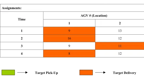
that location. On solving this model, the solution obtained is tabulated in Table 4.

Table 4: Model Optimality – Without Collision Prevention and Target Constraints

Assignments:

AGV # (Location) Time

1 2

1 9 13

2 16 12

3 9 11

4 8 12

Target Pick-Up Target Delivery

The results from Table 4 show that all the targets have been delivered even before they are

picked up. This necessitates the addition of a constraint that restricts target delivery only after

pickup. The model was re-solved with the addition of constraints 7A and 7B. The results of the

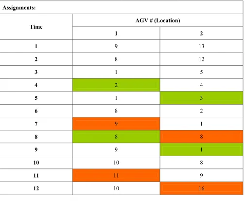
simulation are tabulated in Table 5.

Table 5: Model Optimality – Without Collision Prevention Constraints

Assignments:

AGV # (Location) Time

1 2

1 9 13

2 8 12

3 1 5

4 2 4

5 1 3

6 8 2

7 9 1

8 8 8

9 9 1

10 10 8

11 11 9

12 10 16

Target Pick-Up Target Delivery

From Table 4, we observe that at time 8, both the AGV are at the same grid. Hence, for proving

model optimality, it is essential that the formulation include collision prevention constraints.

The optimal solution is tabulated in Table 6.

Table 6: Model Optimality – Complete Formulation

Assignments:

AGV # (Location) Time

1 2

1 9 13

2 8 12

3 1 5

4 2 4

5 1 3

6 8 2

7 9 1

8 9 8

9 8 1

10 9 8

11 10 9

12 11 16

Target Pick-Up Target Delivery

5.2 Phase II - Heuristic Development – Preliminary Analysis

The following sections compare the functionality of the different heuristic approaches

(detailed in Section 4.2.2) using examples having similar set of input parameters. To illustrate

these approaches, we consider four (4) randomly selected sample problems, with their domains

described in Table 7. The results of this exercise are discussed in Table 8.

Table 7: Heuristic Approaches - Sample Examples – Data

Problem No. Grid Size No. of P/D No. of AGV

1 25 8 2

2 25 6 2

3 36 10 4

4 64 7 4

For the two (2) 25-grid problems, the same layout was selected. For output purposes, average %

of loaded travel for all the AGV combined is also considered. This measure in conjunction with

the total transportation time was used to gauge the heuristic performance.

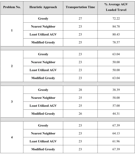
Table 8: Heuristic Approaches - Sample Examples – Results

Problem No. Heuristic Approach Transportation Time % Average AGV Loaded Travel

Greedy 27 72.22

Nearest Neighbor 23 84.78

Least Utilized AGV 23 80.43

1

Modified Greedy 25 78.57

Greedy 23 63.04

Nearest Neighbor 23 50.00

Least Utilized AGV 23 50.00

2

Modified Greedy 23 63.04

Greedy 28 38.39

Nearest Neighbor 25 58.00

Least Utilized AGV 25 57.00

3

Modified Greedy 26 44.31

Greedy 23 67.39

Nearest Neighbor 23 64.13

Least Utilized AGV 23 61.96

4

Modified Greedy 23 67.39

Based on the results in Table 8, the following were the selected observations and next steps:

• Each heuristic has its own unique mechanism of selecting the initial assignments. It is not

possible to observe trends in % AGV loaded travel or the transportation time by looking at a

few sample examples.

• Based on the preliminary heuristic studies, it was decided to also investigate a fifth heuristic

that would be a combination of the 4 heuristics that are listed.

• Detailed experimental designs were required to differentiate between the heuristic

performances, and to compare them with the optimal routes. The following sections

discuss the results from these studies.

5.3 Phase III: Design of Experiments for Heuristic Comparisons / Selection

As discussed in the problem statement (Chapter 2), this work develops optimization

approaches for effectively and efficiently routing AGV in material-handling applications. This

section specifically discusses the methods used in the comparison of the developed optimization

heuristic algorithms. Experimental design methods are used for data gathering purposes, and

statistical techniques are used for solution analysis.

The goal of the experimental designs was to determine a heuristic approach that is robust

across systems, one that can be used in any problem domain irrespective of the number of AGV

or the number of pick-up/delivery (P/D) stations. Two (2) sets of experiments were conducted in

this phase in order to evaluate and compare the performance of the different heuristics. Each

experimental study was a four (4)-step process as discussed by Richardson et al. (2005). These

steps are described below:

Step 1: The controlling factors were identified and their levels decided. The factor levels were bracketed to encompass a practically applicable data range.

Step 2: The second step in the experimental study was to develop a hypothesis based on scientific reasoning to guide decisions on the type and amount of data required to

detect a significant difference. The other activities in this step included deciding

the significance level for testing and the sample size needed for the design to

have adequate power to detect a practically meaningful difference. For practical

purposes, a significance level (p-value) of 0.05 was set. In order to increase the

power of the statistical tests, it was important to decide on the sample size.

Step 3: In the third step of each experimental study, an appropriate statistical test for the data analysis was determined.

Step 4: In the final step of the process, the results of the statistical testing were interpreted to identify statistically significant differences.

The experimental studies are presented in the following sections, and specifically investigate the

results from the experimental designs used in the comparison of the heuristic algorithms. The

statistical differences in the heuristic performance (as measured by its offset from the optimal

solution for small systems, and measured as upper bounds for larger systems) are analyzed as a

function of the system layout, the number of vehicles in the system, and the number of P/D under

consideration.

5.3.1 Experiment Set # 1: Non-Independent Responses

5.3.1.1 Objective: To determine if there was a difference between the 4 heuristics.

5.3.1.2 Design Considerations:

• In order to account for variability across systems, guide path layout was selected as a

“Blocking” factor.

• Responses (solutions from the different heuristics) were non-independent.

• 48 experiments per heuristic – each heuristic tested for same set of AGV starting position

& pickup – delivery (P/D) locations.

• No randomization introduced in the AGV starting position & P/D locations.

5.3.1.3 Factors Evaluated:

• Number of AGV in the system (Factor A) – 2 levels (2 & 3 AGVs).

• Number of pickup/delivery (P/D) stations (Factor B) – 2 levels (4 & 8 P/D).

• Type of Heuristic used to estimate the upper bound (Factor C) – 5 heuristics.

• In order to account for variability across system guide path layouts, a fourth factor called as

“System” is used as a blocking factor (Factor D) – 3 levels. We are only interested in the

main effects of this factor, and would essentially ignore its interaction effects with other

factors.

• 4 replicates (different AGV starting position & P/D location) per system.

5.3.1.4 Layout:

The selection of appropriate system layouts (defined by the guide path design) was

critical in the validity of the experimental design. The methodology used by Beamon et al.,

(1998) for layout selection was used as a guideline for this study.

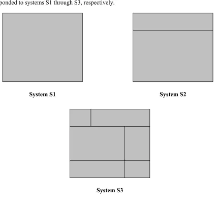
For the experimental design, three material handling system layouts were considered.

These were denoted as System S1, System S2 and System S3. All the three systems allowed for

bi-directional travel. System S1 is a single loop; System S2 is a single loop containing one

cutover, and System S3 is a single loop containing two horizontal and two vertical cut-overs.

The system layouts are shown in F