Graphical visualization of control system performance

(1)

Rochester Institute of Technology

RIT Scholar Works

Theses

Thesis/Dissertation Collections

5-10-1996

Graphical visualization of control system

performance

Jeffrey Marx

Follow this and additional works at:

http://scholarworks.rit.edu/theses

This Thesis is brought to you for free and open access by the Thesis/Dissertation Collections at RIT Scholar Works. It has been accepted for inclusion

in Theses by an authorized administrator of RIT Scholar Works. For more information, please contact

[email protected].

Recommended Citation

(2)

Graphical Visualization of Control System

Performance

A Thesis Submitted

in

Partial Fulfillment of the Requirements for

Masters of Science Degree

in ..Mechanical Engineering

at Rochester Institute ofTechnology

on May 10,1996

By

Jeffrey D. Marx

Approvals:

Dr. Charles Haines, Department Head

Dr. Mark H. Kempski, Thesis Advisor

Dr. Kevin Kochersberger, Thesis Committee

(3)

I, Jeffrey David Marx, grant permission to the Wallace Memorial Library to

reproduce my thesis in whole or in part. Any reproduction will not be for commercial use

or profit.

1/5"/9e:.

(4)

Table

of

Contents

Table

of

Contents

Abstract

1.

Background

and

Introduction

to

Program

1

.

1

Background

1

.2

Purpose

and

Overview

5

1.3

'Visual'

Program Introduction

6

2.

Control

System

Analysis

and

Design

2. 1

Tutorial Overview

20

2.2

Open

Loop

Control

21

2.3

Unity

Feedback Proportional

Control

23

2.4

Proportional

Control

with

Velocity

Feedback

30

2.5

Proportional-Integral

Control

37

3. M-file Descriptions

3

.

1

System Parameter Determination

with

M-file Jl

.m

47

3.2

System Pole

Plotting

with

M-file

J2.m

53

3

.3

Graphical User

Interface using M-file J3

.m

55

3.4

Bode Amplitude

and

Phase Determination

Using

M-files J4.m

&

J5.m

58

3.5

User Pole Selection

with

M-file J7.m

61

3.6

Two-Dimensional

System Time Domain Response

with

M-file

J8.m

63

3.7

Two-Dimensional

System

Bode Response

with

M-files

J9.m

& JlO.m

65

3.8

Two-Dimensional

Response Superposition

with

M-file

Jl 3.

m

67

(5)

3.10

User

Selection

of

Gain Values

for Open

Loop

Systems

with

M-file Jl 5

75

3.11

System

DC Gain Determination

with

M-file

Jl 6m

77

3.12

Root

Locus

Plot Design

Limits

with

M-file

Jl 7.m

78

Appendix

A

Derivation

of

Second

Order Performance

Statistics

Appendix B

Simulink Tutorial

Appendix

C

Theory

Behind Matlab

Step

Algorithm

Appendix

D

M-file

Flowcharts

Appendix

E

M-file Program Codes

(6)

Abstract

University

courses oncontrol system

design have

traditionally

reliedonthe root

locus

approach topredicttransient system output.

However,

the

increasing

speed of

personal computers

has

made

it

practical to

design

control systems

by

simulating

their

time and

frequency

responses.

This

thesis presentsan

interactive Matlab

program

for

control system analysis and

design. The

system

is defined

in

Simulink

with a

user-specified gain parameter of variable magnitude.

The

gain parameter

is automatically

varied

by

theprogramwithin user-specified

bounds. Several

surface and performance

plots are produced which

describe

systemtime-domainand

frequency-domain

performance.

The

systemroot

locus is

alsopresentedwith pole

loci corresponding

to the

gain valuesunderscrutiny.

The

locus

ata specific gain value can

be

selected

for

determination

of systemperformance

using

standard assessmentparameters.

This

programcan

be

applied

in both

an educational

setting

and as a

design

tool

for practicing

(7)

Chapter

1

Background

&

(8)

1.1

Background

Scientific

visualization

is

the

process of

making

complex states ofbehavior

comprehensible

to the

human

eye.

It

has

evolved

from

being

an academic concept

in

the

early 1960's

to

become

a standard part of

engineering

today.

In

its

early

stages, the

expense of computergraphicsequipment

limited

its

use

primarily

to

large

industries

who

could afford

to

invest in

the

equipment.

However,

as

the

cost of computer

hardware

has

decreased,

and

the

sophistication of visualization software

has

increased,

it has become

more cost effective

for

a

broader

range of users.

Human

perception

is

naturally

geared

towards the three

dimensions

of physical

space,

and can

easily

adapt

to

a

fourth dimension

such as color variation.

By

taking

advantage ofthenatural capabilities ofthe

human

eye,

complex results

from

scientific

analysis can

be

communicated efficiently.

In addition,

with

the

use ofhighspeed

computers,

it is

possible

to

display

the

variationof

behavior

over

time

in

animated

sequences which are not captured well

in

print.

Animation

can also

be

used

to

interactively

explore

the

nature of a result

field

by

changing

the

observers view or

zooming

in

on a particular area of

interest.

Many

engineering

design

and analysis applications share common components of

modeling,

analysis,

andvisualizationof results.

The

figure below illustrates

this

process.

(9)

By

creating

a computer model of

the

product or process

being

designed,

it is

possible

to

simultaneously

design,

test,

and

modify

objects

by

computer simulation.

This

current

trend

towardsan

integrated

design,

analysis,

_{and visualization environment}

has

the

following

advantages:

Decreased Physical Testing.

Testing

by

computer simulation

instead

ofactual

prototype

testing

can result

in

a substantial cost savings.

In addition,

it

allows an engineer

to

observe phenomena which might

be dangerous

or

impossible

to

reproduce physically.

Integration

of

Design

and

Analysis. The better

one can visualize analysis

results,

the

easier

it is

to

correct

flaws

shown

by

the

analysis.

Design Optimization.

By

visualizing

analysis results of a model over a range of

parametric

variations,

optimal values

for

the

parameters can

be

more

easily

determined.

Overall,

visualization

techniques

have become

part of a

larger,

evolutionary

trend

in

the

engineering design

field.

Here,

the

computing

environment promotes an

interactive

processwhichencourages

the

exploration of

design

alternatives.

The

goal of

this thesis

is

to

develop

a computer visualization

tool

for

designing

control systems.

However,

this

is

not

the

first

time

this

has been

attempted.

Stephen

Boyd

at

Stanford

University

developed

the

Interactive Control Design Module

(ICDM)

(Boyd,

1993).

His

programshares some of

the

same

features

and

ideas

that

are present

in

the

program

developed for

this

thesis.

For

example, the

main

function

of

both

programs

is

the

interactive design

ofcontinuous-timesingle-input single-output

linear

time

invariant

control systems.

Where

it is

assumed

that the

user

has been

exposed

to the

concepts of

(10)

interface

which makes

them

easy

to

learn

and use.

Also,

they

both

rununderother

software packages.

Boyd's

runs under

Xmath

and mineunder

Matlab. Both

also use a

multiple window

design

where each of

the

windows performs a particular set of

functions.

There

are

however

several

features

which

ICDM

has

which are not available

in

my

program.

For

instance,

ICDM

offers multiple controller

types

and synthesis

methods,

where as

my

program

only

offers

two

(3-D

and

Root Locus).

The

controllers and

synthesis methods offered

by

ICDM

are:

1)

PID

2)

Linear

Quadratic Gaussian

(LQG)

3)

Minimum

Entropy

Controller

(LEQG) 4)

Root Locus.

The

root

locus

controller

synthesis window

features

the

separation,

by

color,

of plant and controller poles and zeros.

It

also allows

the

user

to

graphically

add or

delete

controller poles and zeros.

Another

feature

of

ICDM

is

the

ability

to

study

the

robustness of a controller

to

variations

in

the

plant.

Thus

enabling

the

user

to

compare

the

effect on

the

systems performance

to the

nominal system.

ICDM

also

has

an on-line

help

system

built into it.

Thus,

giving

the

user

a convenient

way

to

find

answers

to

specific questions.

There

arealso several

features

that

are present

in my

programwhichare not

available

in

ICDM. The

first is

the

ability

to

create non-standard control system

configurations.

My

program can

link

with

any

control system

that

is

created

in Simulink

(Matlab's

graphical

block diagram builder).

However,

ICDM

is limited

to

a standard

simple

feedback

control configuration.

Another

advantage

my

program offers

is

the

ability

to

create

3-D

surface plots ofthe systems response over a user-input variable gain

range.

This

variable gain

block

can

be

placed at an

arbitrary

location

within

the

control

(11)

locus

plot

based

on

the

user

input

constraints

for

the

settling

time

andpercent

overshoot.

Another

convenient

feature

of

my

program

is it

will compute

the

performance

statistics of

the

systems

output,

both

analytically

and numerically.

Both ICDM

and

my

programare effective

tools

for

control system

design,

but

(12)

1.2

Purpose

and

Overview

The

scopeof

this thesis

is

to

develop

a

flexible

and

easy

to

use program within

Matlab

thatcan

be

used

to

visualize and analyze

arbitrary

dynamic

systems entered

in

block

diagram

form in Simulink (see

Appendix 'B'). In

particular,

it

was

desired

to

3-dimensionally

visualize

how

the time-domain

and

frequency-domain

response of an

arbitrary

system changed

due

to

a variable gain

block

placed somewhere within

the

block

diagram.

It

was also

desired

that these

3

-dimensionalvisualizations

be linked

together

with

the traditional

root

locus

approach of

analyzing

control systems.

This

program

could

then

be

usedas aneducationalaid

for

system

dynamics

and control systems

courses.

The

programthatwas

developed,

named

'Visual',

was successful

in

meeting

and

going beyond

the

above objectives.

It

can

be

usedas an effective

tool

for both

analysis

and

design

of control systems.

An

educational

benefit

of

the

program

is it

allows

the

user

to

quickly

flip

back

and

forth between

the

root

locus

plot and

the

3-dimensional

response

visualizations.

By flipping

back

and

forth,

students and

practicing

engineers,

can

develop

a

better

understanding

of

how

gainparametervariations affect

the

root

locus

and system

response.

Another

educational

benefit is

that the colorful,

3

-dimensionalresponse

visualizationsare

interesting

to

look

at.

This

visual stimulation will

help

to

increase

student

interest

in

course material.

The

Visual

program also provides an effective environment

for

controlsystem

(13)

theuser

to

manipulate

the

control system

configuration,

as well as changeparameters

within

the

blocks. The

programthen

takes

care of all

the

mathematical and

computational

work,

which allows

the

user

to

concentrate on

the

design

process.

In

addition,

the program

has

an

easy

to

usegraphical

interface,

which allows

the

user

to

issue

commands

by

pointing

and

clicking

on pull

down

menus.

It is

also

interactive

allowing

theuser

to

vary

the

simulation

time,

gain range and

interval,

andperformance

constraintson

the

system.

The

Visual

program

is

also platform

independent because

the

Matlab language

within which

it

was

written,

is

available

for

multiple computer

architectures..

1.3

'Visual'

Program Introduction

The

'Visual'

program

begins

by

creating

a

dialog

box

which promptstheuser

to

select acontrol

system,

previously

created

in

Simulink,

to

be

analyzed.

After

a system

has

been

selectedtheprogram prompts

the

user

to

input

the

simulation

time,

thegain

interval,

and theperformanceconstraints

for

percentovershoot and

settling

time.

The

program

then

createsthree

figure

windows:

3-D,

Root

Locus,

and

2-D. 3-D

is

usedto

create

the

3

-dimensionalresponse visualizations.

Root Locus

is

a window

for functions

pertaining

to the

root

locus

of

the

system.

2-D

creates

2-dimensional

response plots and

computes performance statistics

based

onthesystemresponseplots.

Each

figure

window

has

its

ownset ofmenusand

functions.

The functions

are accessed

by

clicking

and

dragging

menuswhichappear

along

the

top

of

the

window

(i.e.

in

a menu

bar). The

(14)

1.3.1

3-D WINDOW

Output->Amplitude

This

function is

used

to

create a

3

-dimensionalplot of

the time

responseof

the

system over a specifiedgain range.

The

output variable

is

on one

axis, time

is

onthe

second,

and

the

varied gain

is

on

the

third

(see Figure

1.3.1.1).

The

gain range and

increment is input

by

the

user.

A pop-up

menu

in

the

bottom

corner of

the

figure

window

controls whether

the

input is

a

step

or

impulse function. This function is

useful

in

helping

students

better

understand

how

a

changing

gain

block

within a system affects

the

time

domain

response ofa system.

Amplitude PlotwithVariableGain

(15)

Output->Bode(AR)

This

function is

used

to

create a

3-dimensional

Bode Amplitude

Ratio

plot over a

specified gain range.

The

amplitude ratio

is

on one

axis, the

frequency

is

ona second

(log-scale),

and

the

varied gain

is

on athird

(see Figure

1

.3.

1

.2).

Again,

thegain range

and

increment

are

input

by

the user.

A pop-up

menu

in

the

bottom

corner ofthe

figure

windowcontrols whether

the

frequency

unitsare

in

rad/sec or

Hz.

This

function is

useful

in

helping

studentsunderstand

how

a

varying

gain

block

within a system can effect

its

frequency

response.

freq

(rad/sec)

10

2

1

Gain

(16)

Output->Bode(Phase)

This

function

is

similar

to

Bode(AR).

It

is

used

to

producea

3-D

Bode(Phase)

plot overaspecifiedgain range

(see

Figure

1.3.1.3). Again

the

frequency

unitsare

controlled

by

a

pop-up

menu.

This

function is

also useful

for

exploring how

a

varying

gain

block

withina system can effect

its

frequency

response.

freq

(rad/sec)

Gain

Figure 1.3.1.3

View->2D1

This

function

convertsa

3-D

plot

into

a

2-D

plot

for

eachof

the three

previously

described 3-D functions.

It does

this

by

placing

the

view angle parallel with one of

the

(17)

is

given a value of zero

degrees

and

the

elevation angle

is

set

to

zero(see

Figure 1.3.1.4).

This

function is

useful

because

the

2-dimensional

perspectivecan often

clarify information

,

both

qualitative and

quantitative,

from

the

3-D

plots.

View-2D2

This

function

works

the

same as

View-2D1

except

the

azimuth angle

is

given a

value ofzero

degrees(see

Figure 1.3.1.4).

J*

U. -_:i*S^*;%!* .:

"^.^v^-^r^. ::J^

/ Azimuth=-37.5degrees

/ ₇

&

%-^<-i-/;AElevation=_{30 degrees}

Figure 1.3.1.4

1.3.2

ROOT LOCUS WINDOW

Function->Plot

Root

Locus

This function

creates a

locus

plotof

the

poles of

the

closed

loop

transfer

function

of

the

systemunder

scrutiny

(see

Figure 1.3.2.1). At

eachgain

value,

over

the

interval

specified

by

the

user, the

poles are plotted as yellowx's

in

the

real-imaginary

ors-plane.

By

changing

the

gain

interval

the

usercan control

how many

poles are plotted as well as

(18)

Root Locus 0*,

C..D i 1 r ^ 1

X

1 1 1

2

-X

-1.5 X .

1 X

X

.se 0.5

3

-

-66i

0 X X X X X X X X X XX

--

--1 - _X

X X _v

x x_x:

-1.5 ~

X

--2 - X

X

-,5 <;

1 1 1 VI 1 1 1

-5.5 -5 -4.5 -3.5 -3 -2.5 -2 RealAxis

-1.5 -1 -0.5

Figure

1.3.2.1

Function->Select

Gain

This function

is

used

to

selecta particular gain value

from

the

interval

specified

by

the

user.

By

clicking

on a

pole,

or yellow x

in

the

root

locus

plot,

the gain

that

corresponds

to that

particularpole

is

stored

by

the

program and

displayed

in

the

lower

corner ofthe

Root Locus

window.

The

systemcanthen

be

analyzed at

this

gain value.

Function->Gain

vs.

DC Gain

This

function

createsa

2-dimensional

plot of

the

varied gain versusthe

DC Gain

or

steady

state of

the

system.

This

function is

useful

for

determining

the

gain value

that

(19)

Function->Plot

Desired

Region

This

function is

used

to

plot

the

limit lines

of

the

desired

region on

the

root

locus

plot,

based

on a second order approximation of

the

system.

The limit lines

are overlaid

onthe root

locus

plot which must

be

active

in

the

Root

Locus

window

before

this

function

can

be

called.

The

desired

region

limit lines

are

determined based

onthe

constraints

for

percent overshootand

settling

time

of

the

system

(see Figure

3.18,

Franklin (1994)).

If

the

poles of

the

system

lie

within

this region, then

it is

likely

that the

performanceconstraints

for

percent overshootand

settling

time

will

be

met.

Root Locus

6-

4-2

w x

<

co

₀

c O) 3

E

-2

-4

--6

--8 -5.5

: X

X X X X

#

X~~

X X X X

X X XX

x. x x x;:

-4.5 -3.5 -3

Real

Axis

2.5 -1.5 -1 -0.5

(20)

Function->Select

Open

Loop

Gain

This

function

was created

to

allow

the

user

to

select a particulargain

value,

from

the

gain

interval,

in

an open

loop

system.

Because

the

root

locus

of anopen

loop

system

consists of

only

oneset of

poles,

it

is

not possible

to

use

the

'Select

Gain'

function

to

select an

arbitrary

gain value.

By

selecting

this

function,

an

arbitrary

gain value can

be

entered

in

the

Command

windowas

long

as

it is

contained

in

the

gain

interval

defined

by

the

user.

Function->Plot 2-D Response

Once

a gain

has been

selected

from

the

root

locus,

this

function

can

be

used

to

highlight

the

response curve

for

the

selected gain

in

the

3-D

window.

The 3-D

window

is

automatically

made active and

the

response curve

is highlighted in

green against a mauve

colormap

of

the

3-D

surface response plot.

The

3-D

response plot

that

was

last

created

(Amplitude,

Bode(AR),

or

Bode(Phase))

is

the

one used

by

this

function.

This

function

helps

theuserto

determine

wheretheresponse

corresponding

to the

selected gain occurs

within

the

3-D

surface plot..

1.3.3

2-D

WINDOW

Output->Amplitude

This function

is

used

to

output

the time

domain

amplitude response at a gain value

previously

selected

in

the

Root Locus

window

(see

Figure 1.3.3.1). The

time

interval is

the

same as used

for

the

3-D->Amplitude

response plot.

By

plotting

the

amplitude

(21)

Amplitude

Response

3 4

time

(sec)

Output->Bode(AR)

Figure

1.3.3.1

This

function

creates a

2-D

Bode

(Amplitude

Ratio)

plot

using

the

gain value

selected

in

the

Root

Locus

window

(see Figure 1.3.3.2). The

frequency

range

is from

1

rad/sec

to

100

rad/sec.

Again,

the

2-D

plotallows

the

user

to

quantitatively

analyze

the

(22)

0

-20

BodeAmplitudeResponse

-

^X

'

s -to o

-

\

o

\

-80

\

-100 U.S.

:

. :\

10"' 10" 10'

frequency (rad/sec)

10

Figure 1.3.3.2

Output->Bode(Phase)

This

function

worksthe same as

Bode(AR)

except a

Bode(Phase)

plot

is

created

(see

Figure

1.3.3.3).

Bode Phase Response

10"

10 frequency(rad/sec)

10

(23)

Output->Statistics

This function

is

used

to

output

the

performance statisticsof

the

2-D

response plot

that

is

currently

displayed in

the

2-D

window.

A

2-D

response plot must

first

be

created

for

this

function

to work.

All

the

statistics are

determined

numerically using

theresponse

data

except

for first

and second order systems where

the

statistics areestimated

analytically

using

the

natural

frequency,

damping

ratio,

and

time

constant.

For

each of

the

2-D

response plots

the

statisticsare as

follows:

First Order;

Gain

Second Order:

Gain

Settling

Time

Higher Order:

Gain

Rise Time

Amplitude

Break

Frequency

Time

constant

DC

Gain

DC Gain

Peak

Time

Rise Time

Percent Overshoot

Damping

Ratio

Natural

Frequency

Peak Time

Settling

Time

Percent Overshoot

DC Gain

Bode

(

AR

and

Phase)

First Order:

Gain

Second Order:

Gain

Peak

Frequency

Higher Order:

Band Width

Cut-Off Rate

Max Phase Angle

Natural

Frequency

Damping

Ratio

Band Width

Cut-Off Rate

Max Phase Angle

(24)

2

Control System Analysis

and

Design

This

section

is

a

tutorial

on

how

the

program can

be

used as

both

an educational

and

design

tool.

The design

method used

in

the tutorial

is

an enhanced root

locus

method.

This

method combines

the traditional

root

locus

approach withthree

dimensional

visualization

techniques.

First,

a short

description

of

the

Root

Locus

method.

The

Root

Locus

method

is

an outward

design

approach

(Chen,

1993). It

starts

outward withan

initial

design

configuration,

and works

inward

by

adjusting

the

parameters of the components of

the

system until a suitable configuration

is

achieved.

It

is

atrialand errorapproach

to

design

which requires

the

designer

to

"play"with

the

componentsof

the

system.

The

method starts

by determining

the

overall

transfer

function

of

the

system.

The

roots of

the

denominator

of

this transfer

function

are called

poles,

andare

then

plotted

in

the

real-imaginary

plane or s-plane.

By

varying

a

componentof this

system,

such as a

gain, the

systempoles will change

their

s-plane

location. A Root Locus

is

a plot of

the

changing

poles

in

the

s-plane as a gain parameter

changes.

Once

the

Root

Locus

has

been

plotted,

it is

easy

to

determine

a s-plane region

that the

poles must

fall

within

to

meet

the

design

constraintson

settling

time

and percent

overshoot

(Figure

1

.3.2.2).

It

is

then

the

job

of

the

designer

to

find

to

a particular gain

value suchthat

the corresponding

poles

lie

within

the

desired

region.

With

the

poles

known,

the

system responsecan

be

simulatedeither

analytically,

using

inverse Laplace

(25)

The

'

Visual

'

programenhances

the traditional

Root

Locus

method

by

creating

a

3

-dimensional

locus

plot of

the time

responsesover a specified gain range.

One

axis

is

the

output variableof

interest,

the

second

is time,

and

the third

is

the

varied gain

parameter.

The

gain range that

is

used

to

createthe

three

dimensional

timeresponse

plot,

is

thesame gain range used

to

create

the

Root

Locus

plot.

While

using

the

program

offers studentsseveral advantages over

the traditional

Root Locus technique,

it

is

not

intended

as a replacement

for it. Students

still need

to

learn

the

theory

and mathematics

behind

the

traditional methods.

The

program can

then

serve

to

reinforce

these

concepts,

as well as provide an efficient environment

for design.

The

advantages of

using

the

Visual

program overthe

traditional

root

locus

methods can

be divided into

two

categories: education and

design. One

of

the

educational

benefits

of

using

the

program

is

the

ability

to

quickly

flip

back

and

forth

between

theroot

locus

windowand

the

3

-dimensional

time

response

locus

window.

By

flipping

back

and

forth,

students can

develop

an

intuitive

feel for how

the

changing

s-domain

pole

locations

effect

the time

domain

system response.

Another

educational

benefit

oftheprogram

is

that the

3-D

visualizationof

the time

responses

is

more

visually

stimulating

to

students

than the

2-D

root

locus

plot.

This

visual stimulation will

help

to

keep

students attention

focused

on

the

subject matter.

The Visual

program also provides an effective environment

for

control system

design.

Because

the

program

interfaces

with control systems

defined

as

Simulink

block

(26)

systemconfiguration.

In

addition, the

Visual

program

takes

care of all

the

mathematical

and computational

work,

allowing

theuser

to

concentrate on

the

design

process.

This

fascilitates

the

user

being

able

to

"play" with

the

design,

without

getting bogged down in

mathematics at each step.

The Visual

program also overcomes several ofthe

limitations

of

the

root

locus

design

method.

One limitation is

that

the

desired

region on

the

root

locus

plot

is

only

a

rough estimate

for

systems of order

higher

than two

(Chen,

1993).

In

these

cases

the

systemresponseshould

be

numerically

simulated

to

ensure

that

the

design

constraints

have been

met.

Since,

the

program

automatically

simulates

the

response

numerically, the

user

has

a quick

way

to

check whether

the

desired

region

is

valid

for

a paticular system of

poles.

If

the

user

is

dealing

with a complex

system,

with perhaps

4

or more

branches

going

in

various

directions,

it

may

be difficult

to

interpret how

the

root

locus

affects

the

time

domain

response.

By

using

the

3-D

timeresponse windowwithin

Visual,

it is

easy

to

qualitatively

understand

how

the

systems

time

response

is

affected

by

the

gain change.

Another limitation

encountered

in

the

root

locus

technique

is

that

the

design

constraint on

the

steady

state error

is

usually

ommitted

from

consideration.

By

using

the

Visual

programs

3-D

window, the

user

is

able

to

visualize

how

the

steady

state error varies with

the gain,

as

long

as

the

response

has

been

simulated

beyond

the

steady

state point.

A

final design

advantageof

using Visual

is it

allows

the

user

to

specify

thegain range over

which

to

analyze

the

system.

By

specifying

asmallerand smaller gain

range, the

user

(27)

2.1

Tutorial

Overview

In

this tutorial

we will

look

at

three

different

control scenarios:

1)

Proportional

control

2)

Proportional

control with

velocity

feedback

3)

control.

The first

scenario

is

proportional control with

unity

feedback,

of a simple

two

lag

plant.

The

plant

transfer

function is:

1

G(s)

=

(s

+

4)(s-.5)

s2+3.5s-2

It

could

be

the transfer

function

of a motor

driving

a

load. The block diagram for

this

control system was

defined

in

the

Simulink

tutorial

as

Prop.m.

It

should

be

ofthe

form:

1

+

Surr

K

1

y

npor

t

s^+3.5s-2

Plant

F

igure

2. 1.1

Say,

the

control

design

must

be

able

to

meetthe

following

constraints:

Position Error

<=

20%

Overshoot

<=

20%

Rise Time

<=

0.5

_sec.

Settling

Time

<=

3

sec.

The

goal of

the

designer

is

to

find

aproportionalgain

(K)

such

that

all

the

design

(28)

Prior

to

launching

the

Visual

program,

the

controlsystem

designer

may

wish

to

define

root-locusconstraints

using

equivalentsecond order system response criteria.

The

settling

timeconstraint would

dictate

a

lower bound for

a)n

and

hence,

pole real-axis

location.

Likewise,

the

overshoot constraint would

dictate

a max and

hence,

define

an

admissible wedge-shapedregion of

the

s-plane

(Figure

1.3.2.2).

The

damping

ratio

(Q

thatcorresponds

to

the

design

constraint

for

percent

overshoot,

can

be

determined

from

Figure 2.1.2. The

damping

ratio

that

corresponds

to

a percent overshoot of

20

percent

is

approximately 0.46. The Visual

program

automatically

determines

the

desired

pole

region

from

the

user supplied

information.

1UU

-

80

c u

i

60

o o

-

40

>

O

20

0

0.2

0.4

0.6

0.8

1.0

1.2

Damping

ratio

Figure 2.1.2

2.2

Open

Loop

Control

(29)

^

Make

the

Visual folder

theactive path

by

opening

the

Visual folder

and

then

hitting

thecancel

button (or

edit

the

Matlab

Path

^

First let's

try

open

loop

control of

the

system.

Type

"Visual'

in

the

Command

windowto start

the

program.

When

the

dialog

box

appears,

chosethe system

"open.m".

Enter

the

correct

transfer

function

G(s),

in

the

plant

block

as shown

in

Figure 2.2.1 (Refer

to

the

tutorial

in

Appendix

'B' as

needed.)

1

npo

fe.

K

1

>w 1

y

1

3^+3.58-2

w

Figv

Plant

ire

2.2.1

^

Click

in

the

Command

window.

#

Enter

an

ending

timeof

7

seconds,

anda

time

increment

of

0.025

seconds.

^

Enter

a

starting

gainof

1

, an

ending

gain of

6,

anda gain

increment

of

0.5.

^

Enter

the

design

constraint

for

the

damping

ratio

(0.46)

and

settling

time

(3

sec).

Three

windows should appearon

the

screen

(3-D, 2-D,

and

Root

Locus).

2.2.1

Time-Domain

Response

^

In

the

'3-D'

window,

underthe 'Output'

menu,

select

'Amplitude'

(Abbreviated;

(30)

The step

response

is

unstable

for

all

the

gain values

in

the

selected range.

Increasing

gain

increases

the

speed of

reponse,

but does

not

improve

the

system stability.

This

is

expected

because

the

system contains a pole

in

the

right

half

of

the

s-plane.

2.2.2

Root Loci

^

Make

the

'Root

Locus'

windowactive

by

clicking

in it

with

the

mouse.

^

Root Locus->Function->Plot Root Locus

The

gain

does

not change

the

roots of

the

transfer

function

for

an open

loop

system.

Therefore,

the

root

locus

consists of

the

roots of

the

plant

transfer

function.

Because

there

is

one positive real root at

0.5,

the

system willalways

be

unstable regardless of

the

gain.

Thus,

we cannot achieve

any

of our

design

requirementswith open

loop

control.

2.3

Unity

Feedback

Proportional Control

Let's

try

aunity-feedback

configuration,

withproportional control.

^

Close

all

three

openwindowsexcept

the

Command

window

^

Start

theprogram

by

typing

either,

"Visual'

or

"/3"

J3

starts

the

program

bypassing

the

coverpage.

Choose

"Prop.m",

andenter

the

transfer

function

G(s),

in

the

Plant block

as

defined previously

in

Figure 2.1.1.

^

Click

in

the

Command

window.

^

Enter

a

ending

time

of

7

sec,

and a

time

increment

0.025

sec.

^

Enter

a

starting

gain of

1,

an

ending

gain of

7,

and a gain

increment

of

0.5.

(31)

2.3.1

Time-Domain

Response

+

3-D->Output->Amplitude

Here,

the

responsechanges

from

unstable

to

stable over

the

gain range.

Hence,

closing

the

loop

in

conjunctionwitha proportional gain

has

affected

the

system's stability.

2.3.2

Root Loci

^

Make

the

'Root

Locus'

window active.

^

Root

Locus->Function->Plot Root

Locus

For

a closed

loop

system, the

roots change as

the

gain changes.

The

root

locus

starts with

one unstable root at

0.5.

However,

as

the

gain

is

increased

this

root

is

pulled

into

the

left

half

plane,

making

the

system stable.

This stablizing

effect can also

be

seen

in

the

3-D

window.

^

Root Locus->Function->Select

Point

#

Click

on a polethat corresponds

to

a gain of

1

.

5

.

When

a pole

has

been

selected

it

turns green,

and

the

corresponding

gainvalue

is

displayed in

the

lower

left

corner.

The

Select Gain

pull-down

function

can

be

used

repeatedly

untilthe

desired

gain

has been

selected.

2.3.3

Performance Assessment

^

Root

Locus->Function->Plot

2-D Reponse

Note

that

the

response

corresponding

to the

selected gain

is highlighted in

the

3-D

window.

(32)

The

system

is

unstable

for

that

gain

value, thus the

response

is

unbounded.

+

2-D->Output->Performance Stats

There

is

no stable

DC Gain for

this

root

locus

selection,

thusall

the

other statistics are

meaningless.

The

program recognizes

that the

response

is

unstable and

informs

the

user.

^

Make

the

Root

Locus

window active again.

^

Root Locus->Function->Select Gain

^

Click

on a pole

corresponding

to

a gain of

4.

^

Root Locus->Function->Plot

2-D

Response

+

The

response

is

now stable and

the

output

is

now

bounded.

+

Since

theresponse

is

stable, the

DC Gain

and all other stats are

defined.

Increasing

the

gain

has

made a

dramatic

improvement in

the

performance of

the

system.

However,

the

response

is

still

too

slow

to

meet

the

performance specifications.

Now

let's

see

if

there

is

a

gain,

within

the

range we

specified, that

will

satisfy

all

the

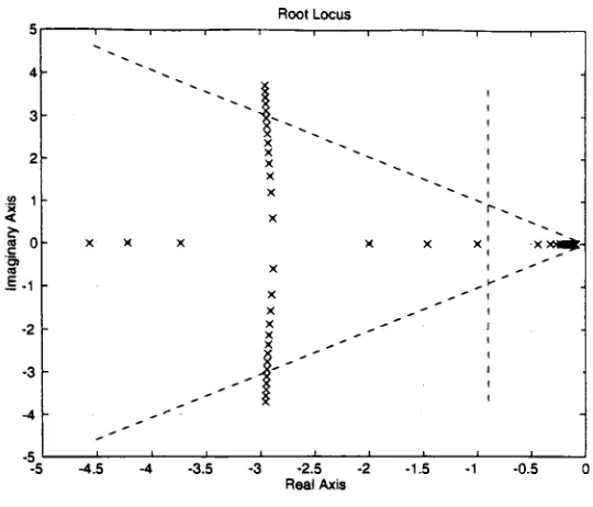
performance criteria.

2.3.4

Proportional Controller

Design

^

Make

the

Root

Locus

windowactive.

Notice

that the two

branches

ofthe

locus

converge at around a gain of

5,

after which

the

branches

continue

in

opposite

imaginary

directions.

Since,

(see Figure

2.3.4.1)

the

settling

time

is

determined

from

the

real part of

the roots, the

settling

time

reaches a

(33)

Root Locus

-2 -1.5

Real Axis

Figure

2.3.4.1

Make

the

3-D

windowactive.

As

expected

the

response

time

seems

to

level

off at around a gain of

5. Also

notice

that

the

response speed

increases

as

the

gain

increases.

+

Click

back

in

the

Root

Locus

window.

^

Root

Locus->Function->Select

Gain

+

Click

on a pole

corresponding

to

a gain of

6

^

Root

2-D

Response

+

2-D->Output->AmplUude

(34)

+

2-D->Output->Performance

Stats

The DC Gain

is

still

too

high

to

meetthespecification.

^

Make

the

3-D

window active

Notice

that theposition error

decreases

asthegain

increases.

Therefore,

we need a gain

greater

than

6

to

meet

the

specification on position error.

^

Close

all

three

open

figure

windows.

^

Type

"J3"

to

runprogram

again,

and choose"Prop.m"

^

Enter

a end

time

of

7

sec,

and a

time

increment

of

0.025

sec.

^

Enter

a

starting

gainof

6,

an

ending

gainof

20,

and a gain

increment

of

0.5.

^

Enter

the

desired

damping

ratio

(0.46),

and

the

desired

settling

time

(3 sec.)

4.

3-D->Outpui->Amplitude

Notice

that

the

steady

state error

decreases

as

the

gain

increases.

*

3-D->View->2-Dl

The

responsecurves are pushedoutwardas

the

gain

increases.

Thus

the

response

is

sloweras the gain

is

increased

and

correspondingly the

rise

time

decreases.

4.

3-D->View->3-D

^

Make

Root Locus

windowactive.

+

Root

Root Locus

+

Root

Desired Region

All

the

poles

fall

within

the

desired

region

for

settling

time.

At

a gain

less

than

16.5

the

(35)

^

Root Locus->Function->Gain

vs.

DC Gain

From

theperformance

criteria,

theposition error must

be less

than

20%. From

thegraph

it

can

be

seenthat

this

criteria

is

met at a proportional gain greaterthan

12.

Thus,

tomeet

both

performance criteria

the

gain needsto

be between

12

and

16.5.

^

Root

Root Locus

^

Root Locus->Function->Select Gain

^

Click

on a pole

corresponding

to

a gain of

12.

^

Root

2-D Response

+

Increasing

the

gain

has

improved

the

steady

state error.

#

Stats

The

specifications

for

DC

Gain,

overshoot,

and

settling

time

have

been

met.

However

rise

time

is

stilltoo slow.

If

you

flip

back

to the

3-D

windowyouwill notice

that

as

the

gain

increases,

the

rise

time

decreases.

Therefore,

weneed

to

increases

the gain

to

decrease

the

rise

time.

^

Make Root Locus

windowactive.

^

Root

Gain

+

Click

on a pole

corresponding to

a gain of

1

6.5.

+

Root

2-D Response

^

(36)

All

the

performancespecifications

for

the

system

have

now

been

met.

Thus,

by

using

a

unity feedback

control

configuration,

with aproportionalgain of

16.5

the

system

design

is

complete.

The

specifications

for

our system are:

Overshoot-

19.68%

Settling

Time

-

2.629

_sec.

Rise

time

-

0.4727

_sec.

DC

Gain

(37)

2.4

Proportional

Control

with

Velocity

Feedback

The

next example we will consider makes use of aproportional-derivitive

controller.

The

plant

transfer

function

we wish

to

control

is:

G(S)=

3

1

2 <

s +6s +5s

which

incorporates

a

free integrator in

the

plant

dynamics.

Let

us assume

the

output of

the

plant

is

a positionsignal.

The

following

have been

specified

for

the

system response.

1. Overshoot

<=

5%

2.

Settling

time

<

5

sec.

3. Rise

time

as smallas possible.

4. Position

error as small as possible.

First,

weneedto

find

the

damping

ratio thatcorresponds

to

the constraint

for

percent

overshoot.

From Figure 2. 1

.2,

the

damping

ratio

that

corresponds

td

a overshoot of

5

percent

is

approximately

0.70. We

will start

the

design

withproportional control.

2.4.1

Proportional

Control

with

Position Feedback

+

Make

the

Visual

folder

the

active

path,

andstart

the

program

by

typing

"J3"

or

"Visual*.

Chose

"Prop.m"

(38)

1 + fe.

w nport

Sum

Figure 2.4.1.1

^

Click in

the

Command

window.

^

Chose

an

ending

time

of

1 1

sec,

and a

time

interval

of

0.025

sec.

#

Chose

a

starting

gain of

1

, an

ending

gain of

1

8,

and a gain

interval

of

1

.

^

Enter

the

constraints onthe

damping

ratio

(0.7)

andthe

settling

time

(5

sec).

+

As

the

gain

increases

the

system

becomes

increasingly

oscillatory

until

it

eventually

becomes

unstable.

#

Make

the

Root

Locus

windowactive.

^

Root Locus->Function->Plot Root Locus

At

a gaingreaterthan

16,

two

of

the

system poles are

in

the

right half

plane which

indicates instability.

^

Root

Desired

Region

No

systemof poles

fall

into

the

desired

region

for

settling

time,

and

for

a gain greater

than

1,

the

poles

fall

outside

the

desired

overshoot region.

+

Root

Gain

(39)

+

Root

Locus->Function->Plot 2-D

Response

+

^

Stats

As

expected

for

again of

1

, even

though the

overshoot meets

the

specification

the

settling

time

is

much

too

large. We

cannot

improve

the

settling

time

with proportional

control,

so

we need

to

try

a

different

control configuration.

2.4.2

Proportional Control

with

Position

and

Velocity

Feedback

Let's

try

a

velocity

feedback

controlconfiguration.

This

configuration

has

two

possible

parameters

to

be

varied, the

proportional

(controller)

and

derivitive

(feedback)

gains.

For

thisscenario optimal values

for

both

gains need

to

be found.

To

accomplish

this

a

constant value will

be

selected

for

the

proportional

gain,

and

the

derivitive

gain will

be

varied over a specified range.

This

process will

be

repeated

using

different

constant

values

for

the proportional gain

in

an

interative fashion. The

velocity

feedback

control

configurationshould

be

of the

form

shown

in

Figure 2.4.2.1.

Inport

D>

Sum

Gainl

Sum1

s'+Ss+S

Plant

<

Integrator

2.4.2.1 Baseline

Configuration

(40)

^

Start

the

program

by

typing "73",

andchoose "Velfeed.m"

^

Enter

the

correct "Plant"

transfer

function block from Figure

2.4.2.

1

.

^

Under

the

derivitive

or

feedback

gain

block,

enter

the

label

"K". Under

the

proportionalgain

block,

enter

the

label

"Prop".

Inside

the

block

enter a value of

1

for

the

proportional gain.

+

Enter

an

ending

time

of

1

0

seconds,

and a

time

increment

of

0.025

sec.

^

Enter

a

starting

gain of

1

, an

ending

gain of

9,

and a gain

increment

of

0.5.

^

Specify

the

damping

ratio

to

be

0.7

and

settling

time

to

be

5

seconds.

^

Ten

seconds

is

not

long

enough

for

the

system

to

reach

steady

state.

We

need

to

increase

the

simulation

ending

time.

Also,

notice

that

increasing

the

derivitive

(feedback)

gain

makes

the

response slower.

^

Make

the

Root

Locus

windowactive.

^

Root

Desired

Region

The

poles

fall

outside

the

desired

region

for

settling

time,

because

there

is

a

dominant

(41)

RootLocus

2.5 -2 Real Axis

[image:41.566.118.388.55.286.2]

1 -0.5 0

Figure 2.4.2.2

#

Click

on a pole

corresponding

to

a gain of

2.5.

^

Root

2-D Response

+

The

response

has

not reached

steady

state.

The final

time

should

be increased.

^

The settling

time

could not

be

computed

numerically because

the response was not

carried out

to

steady

state.

Also

the

rise

time

is

much

too

large.

2.4.2.2 Improved Configuration

Change

the

proportionalgain

to

a value of

5.

^

Close

all

three

open

figure

windows.

(42)

^

Enter

5 in

proportional gain

block

(Prop)

+

Enter

an

ending

time

of

7

sec,

and a

time

interval

of

0.025

sec.

^

Enter

a

starting

gain of

1

, an

ending

gain of

1

0,

and a gain

interval

of

0.

5

.

^

Specify

the

constraintson

the

damping

ratio

(0.7)

and

the

settling

time

(5

sec).

+

3-D->Output->Amplitude

The

response

is

more stable

for

a proportional gain of

5.

Increasing

the

feedback

gain

does

not maketheresponse

become

oscillatory.

*

3-D->View->2-Dl

From

this

two

dimensional

perspective,

it

can

be

seen

that

increasing

the

feedback

gain

makes

the

time

response more sluggish since

the

rise

time

is increasing.

^

Make

the

Root

Locus

window active.

^

Root

Root Locus

#

Root Locus->Function->Plot Desired

Region

The

poles

fall

into

the

desired

overshoot region

if

the

feedback

gain

is

greater

than

3

and

less

than

6.5. The

poles

fall

within

the

desired

settling

time

region

if

the

feedback

gain

is

less

than

5.

Therefore,

to

meet

both

specifications, the

feedback

gain must

be between

3

and

5.

However,

because

the

system

is

of a

higher

order

than

2,

we cannot

be

certain

that

the

system

truly

meetstheconstraints until we simulate

the

systems response.

^

Make

the

3-D

windowactive.

As

predicted

in

the

root

locus

window, the

overshootstarts

high,

then

decreases,

then

(43)

^

Click back in

the

Root

Locus

window.

^

Root

Locus->Function->Select Gain

^

Click

on a pole

corresponding

to

a gain of

3

.

^

Root

2-D

Response

4

The

response appears

fast

and stable.

4

2-D->Output->Performance

Stats

The

criteria

for

the

settling

time

and

the

overshoot

have been

met,

andthe

rise

time

is

1.4

seconds.

Let's

see

if

the

performance statistics can

be improved.

^

Make

the

Root Locus

window active

^

Click

ona pole

corresponding

to againof

4.

^

Root Locus->Function->Plot 2-D Response

+

2-D->Output->Amplitude

There

is

novisibleovershoot.

+

Stats

The

statistics

for

the

overshoot and

settling

time

are stillwithin

the

constraints.

However,

the

rise

time

has been increased

to

1.75

seconds.

There

exists a

trade-off

between

the

rise

time

and

the

overshootas

the

gain

is increased.

If

the

rise

time

is

the

more critical statistic thena gain of

3

should

be

used.

However,

if

the

overshoot

is

the

more

important

(44)

2.5

Control

Example

The

last

example we will

look

at

is

a_{proportional-integral} _{control scenario with}

unity

feedback. The

plant

transfer

function is:

1

G(s)

=

-sz+4s+

3

The

for

the

system are:

1)

Position

error <

10%

2)

Overshoot

<

10%

3) Settling

time

<

3

sec.

4)

Rise

time

<

0.6

sec.

From

Figure

2. 1

.2,

the

damping

ratio

corresponding

to

an overshoot of

10%

is

approximately 0.62.

We

will start

the

design

by

using

a simple

unity

feedback,

proportional control scenario.

2.5.1.1 Baseline Proportional

Control Scenario

^

Make

the

"Visual"

folder

the

active path.

^

Start

program

by

typing "J3",

choose"prop.m"

^

Enter

the

transfer

function

G(s)

in

the

Plant block

from Figure 2.5.1.1.1

(45)

^

Click in

the

commandwindow

+

Enter

a end

time

of

7

sec,

and a

time

interval

of

0.025

sec.

^

Enter

a

starting

gain of

1

, an

ending

gain of

9,

and a gain

interval

of

0. 5

.

+

Enter

the

settling

time

(3 sec.)

and

the

damping

ratio

(0.62)

constraints.

4.

The

response

is

stableand steadies quickly.

The steady

state response of

the

system

increases

as

the

gain

inceases.

^

Make

the

Root Locus

window active.

^

Root

Desired Region

All

the

poles

fall into

the

desired

region

for

settling

time.

For

a gain of

less

than

7.5,

the

poles

fall

within

the

desired

region

for

overshoot.

This

is

consistantwith what

is

observed

in

the

3-D

window.

+

Root

Gain

^

Click

on a pole

corresponding

to

a gain of

8

+

Root

2-D Response

^

There

is

a

large steady

state error at

this

gain value.

4

Stats

The steady

stateresponse

is

0.727. This

is

below

the

requirementof

0.9.

However,

all

(46)

^

Close

all

three

open

figure

windows.

2.5.1.2

'Improved'

Proportional Control Scenario

Let's

try

proportional control

again, this time

using

larger

gains

to

eliminate

the

steady

state error.

+

Type

"73"

to

start

program,

choose"prop.m"

^

Enter

an

ending

time

of

7

sec,

and a

time

interval

of

0.025

sec.

+

Enter

a

starting

gain of

1

0,

an

ending

gain of

34,

and a gain

interval

of

2

^

Enter

the

constraints on

the

damping

ratio and

settling

time.

4

The

steady

state error

is

decreasing,

and

the

response settles

faster

as

the

gain

increases.

However,

the

downside is

the

overshoot also

increases

as

the

gain

increases.

^

Make

the

Root

Locus

window active.

+

Root Locus->Function->Plot

Root

Locus

^

Root

Desired Region

None

of

the

poles

lie

within

the

desired

region

for

overshoot.

However,

they

do fall

within

the

desired

settling

time

region.

^

Root

Locus->Function->Select Pole

Click

on a pole

corresponding

to

a gain of

32.

+

Root

Locus->Function->Plot 2-D

Response

4

(47)

4>

Stats

In

order

to

meet

the

specification on position error

the

overshoot

has

jumped

to

32.35

percent.

Thus,

it is

not possible

to

meet all

the

performance specifications withsimple

proportional control.

2.5.2

P-I

Controller Design

A

different

type

of control configuration must

be

used

that

will meet all

the

transient

performance

criteria,

while also

achieving

good

steady

state performance.

Try

a

control configuration which eliminates

the

steady

state error.

Figure 2.5.2.1

depicts

the

system

block diagram.

Figure

2.5.2.1

This

control scenario

has

two

free

parameters,

K

and

Ki. In

order

to

find

a optimal value

for both

parameters,

we will

arbitrarily

choosea value

for

the

proportional gain

(K)

and

vary

the

integral

gain

(Ki

)

over some range.

This

processwill

be

repeated until values

for K

and

Ki

are

found

that

meet

the

desired

specifications.

2.5.2.1 Baseline P-I Control Scenario

4s

Type

"73"

to

start

program,

and choose

(48)

4

Enter

the

correct

transfer

function

G(s)

in

the

Plant

block

from Figure 2.5.2.

1

4

Name

the

proportionalgain

block

'Prop' and enter avalueof

1

.

4

Name

the

integral

gain

block

'K'.

4

Enter

an

ending

time

of

12

sec,

and a

time

interval

of

0.025

sec.

4

Enter

a

starting

gain of

1

, an

ending

gain of

6,

and a gain

interval

of

0.5.

4

Enter

the

constraints on

the

damping

ratio

(0.62)

and

the

settling

time

(3

sec).

4

The steady

state error

has been

eliminated.

However

as

K,

increases

the

response

becomes

more oscillatory.

4

Make

the

Root

Locus

window active

4

Root

Locus->Function->Plot Root

Locus

4

Root

Locus->Function->Plot Desired Region

None

of

the

poles are within

the

desired

region

for

settling

time.

The

settling

time

is

increasing

as

Ki

increases

because

the

dominant

pole

is moving

towards the

origin.

4

Make

the

3-D

windowactive

As

K

increases

the

response

becomes

more

oscillatory

and

less

settled.

Therefore,

using

1,

the

design

criteriacannot

be

met.

4

Close

all

three

open

figure

windows.

2.5.2.2

'Improved'

P-I

Control Scenario

Try increasing

the

proportional gain

(Prop).

4

Type

"73"

to

start

program,

and choose

(49)

4

In

the

proportional gain

block

(Prop),

enter

4.

4

Enter

an

ending

time

of

9 sec,

and a

time

interval

of

0.025

sec.

4

Enter

a

starting

gain of

1

, an

ending

gain of

6,

and a gain

interval

of

0.5.

4

Enter

the

constraintson

the

damping

ratio

(0.62)

and

settling

time

(3

sec).

4

The

response

is

more stable and

less

oscillatory using

4.

4

Make

the

Root Locus

window active.

4

Root

Locus

4

RootLocus->Function->Plot Desired

Region

The

constraint on

the

settling

time

is

not met.

By

selecting

a particular gain values

for

K

and

plotting

theamplitude response

in

the

2-D

window,

it

can

be

shown

that

as

K

increases,

settling

time

first decreases

until

K

=

4.5,

then

increases.

The

overshoot

continuously

increases

K,

increases. For

4,

no value of

K

can meet

all

the

performance criteria.

4

Close

allthree open

figure

windows.

2.5.2.3

'Refined'

P-I Control

Scenario

Try

increasing

the

proportionalgainagain.

4

Type

"73"

to

run

program,

and choose"Plone.m"

4

In

the

proportional gain

block

(Prop

),

enter

9.

4

Enter

a

ending

time

of

7

sec,

and a

time

increment

of

0.02