Time series recursions and stochastic approximation

(1)

Victor Solo

A thesis submitted for the degree of Doctor of Philosophy

at

(2)

The results presented in this thesis are my own, unless otherwise stated.

(3)

F

on.

(4)

A C K N O W L E D G E M E N T S

It is a pleasure to thank Professor E.J. Hannan for his encouragement and enthusiastic supervision. Thanks too, to Dr P.C. Young, who shared the supervision, for his guidance and persistent reminder of the ’Engineering’ point of view.

I gratefully acknowledge the financial support of a Commonwealth Postgraduate Research Award.

Thanks to my friend Padmini for her good humour.

(5)

ABSTRACT

This thesis is concerned with the asymptotic theory, both convergence and Central Limit Theorem, for recursive estimators of time invariant

parameters in Time Series models. This theory derives from a similar theory for classical Stochastic Approximation schemes so that these too, are given some consideration.

The thesis is divided into two parts. In Part I after an introductory chapter, a general approach is offered for the construction of recursions from a Prediction Error or Gaussian Likelihood viewpoint. This approach also allows other methods (for example, Model Reference) to be seen in context. Next, an heuristic argument is used to intuit the asymptotic properties of a general class of recursions (including the Prediction Error Recursions) and Time Series Stochastic Approximation schemes. The third chapter of Part I contains simulations illustrating some of the above ideas.

In Part II attention is turned to a rigorous analysis of various recursive and Stochastic Approximation schemes. In Chapter 4 a general regression problem is considered and strong convergence proved under various conditions. Chapter 5 is concerned with deriving limit laws for classical Stochastic Approximation in a general setting: in Chapter 6 this is

extended to allow dependent noise. Chapter 7 contains a Central Limit

(6)

L I S T OF F I G U R E S A N D T A B L E S

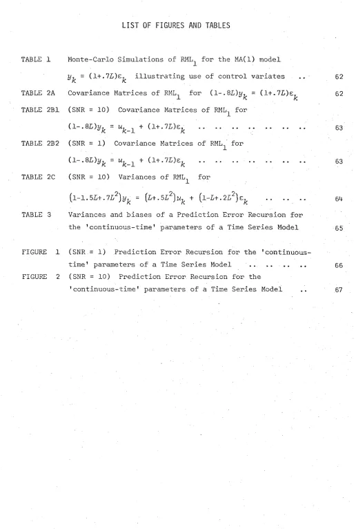
TABLE 1

TABLE 2A TABLE 2B1

TABLE 2B2

TABLE 2C

Monte-Carlo Simulations of RML for the MA(1) model y^ = ( 1 + . 7 i l l u s t r a t i n g use of control variates Covariance Matrices of RML^ for (l-.QL)y^ = (1+.7L)e (SNR = 1 0 ) Covariance Matrices of RML^ for

(1-.8 L)y^ = uj<_-^ + (l+.7L)e^ ... (SNR = 1) Covariance Matrices of RMLn for

(1-.8L)y^ = ^ + (l+.7L)e^ ... (SNR = 10) Variances of RML^ for

(l-1.5L+.7Z,2) ^ = (L+.5L2) ^ + (l-L+.2L2) ... TABLE 3 Variances and biases of a Prediction Error Recursion for

the ’continuous-time* parameters of a Time Series Model

62 62

63

64

65

FIGURE 1 (SNR = 1) Prediction Error Recursion for the

’continuous-time’ parameters of a Time Series Model ... 66 FIGURE 2 (SNR = 10) Prediction Error Recursion for the

[image:8.554.35.551.49.815.2]

(9)

a

V ß>

a. s .

3

CLT

Ca (L)

D, V

ek(0)

V 0) =

IP K-W

L

LIL M-C m . d .s . m. s . o.d.e.

p

lim

RLS RML^

R M L 2 s . d . e . SNR w. l.o. g w . p . 1 w . r .t .

N O T A T I O N

vector of noise parameters Matrix of system parameters

3

almost surely

system parameters Central Limit Theorem

n

c

i

I

C ^ ( a

)L

where

C^.(a)

are matrices of noise parameters

derivative operator

one step ahead prediction error generated by a parametric model

M(Q)

Zy{/kJ M

= - 3 e ^ ( 0 ) / 3 Ö

Invariance Principle (in Chapter 2 infinite past) Kiefer-Wolfowitz

lag or backwards operator Lav/ of the Iterated Logarithm Monte-Carlo

Martingale Difference Sequence mean square

ordinary differential equation limit in probability

limit in probability Recursive Least Squares

Recursive Maximum Likelihood (Recursion) Scheme 1 Recursive Maximum Likelihood (Recursion) Scheme 2 Stochastic Differential Equation

Signal to Noise Ratio without loss of generality with probability one

(10)

P AR T I

P R E A M B L E

This thesis aims to investigate the asymptotic behaviour of Time Series Recursions and Stochastic Approximation (SA) with particular emphasis on the

second order properties, that is, asymptotic variances or Central Limit Theorem: the thesis is divided into two parts. In Part 1 the introductory chapter reviews some basic notions in recursive estimation and indicates, in an informal way, some of the basic ideas of the thesis. The remainder of Part I sacrifices rigour to provide a plausibility analysis of the behaviour of recursions (that is, coyivergence and asymptotic variances) as well as considering ways of constructing them. Some of these ideas are illustrated with simulation studies. In Part II a rigorous analysis is given of the asymptotic properties of some classical Stochastic Approximation schemes

(11)

C H A P T E R 1

I N T R O D U C T I O N

1-1

G e n e r a l

In recent years there has been an enormous interest in recursive

methods of parameter estimation for Time Series models (Astrom and Eykhoff, 1971, Young, 1974). Recursive estimation has been seen as a technique to go hand in hand with real time forecasting (Holst, 1977) or state estimation, to form part of an adaptive control scheme (’Aström and Wittenmark, 1973^, Young and Beck, 1974), to be used in pattern recognition (Kittler and Young, 1973) or to be used as an aid to model building where the parameter variation over an observation interval may suggest a cause of model inadequacy (Young, 1974).

While it seems that Gauss was the first to use recursive methods 0 4 *0)

(Young, 1974), the modern use begins with Plackett.and Kalman (1960). Let us therefore begin with a review of Plackett’s algorithm and some of its extensions.

1.2 R e c u r s i v e L e a s t S q u a r e s

The recursive least squares (RLS) algorithm or Plackett algorithm is a sequential procedure for the computation of the least squares estimator of a regression coefficient. Suppose a sequence of noisy observations is

available on a scalar process

y

^ together with noiseless or error free measurements of a related

m

dimensional process . The process

might be chosen by the data analyst, its components consisting perhaps of sinusoids if

y^

was periodic,or may be part of the environment, with, say, its components

~

j,

where

u

^ is an input sequence into a dynamical system. The aim of regression analysis is to describe the relation between

y

^ and x^ in a linear fashion as

»k = Xk

$0 +

£k

(12)

coefficient in the first example above or an impulse response vector in the second example. The sequence is an error or disturbance sequence. The RLS algorithm may be derived by manipulating the en-bloc estimator or by sequential optimisation of the criterion

N 9

V e) =

% E

v e)

with

= 2/7, • The latter course is taken here. We observe

V S)

=

PN-1

(P)

+

so that, noting de^/d$ = x ,

df>N/d& = dPN_1/d$ -

x ^ ( 3 ) • (1.1)

Further

= ^ V ^ f S ' = d \ _ x/ d m ' + x^x.' so

P-,1 =

y

x. x / .

J /(/: (1.2)

Next, denoting the estimator by 3y , a. Taylor series for dP^/d$^ (- 0) yields

A A

*N ^N-1 W < V l

^ / / - l + *

(1.3)

Now (1.2), (1.3) may be put in fully recursive form by means of the Matrix Inversion Lemma (Bodewig, 1956), that is,

PN

Vl

PN-1XNXNPI1-1/ (1+XNPN-lXl) '

This expression is immediately verified by multiplying on the left by P

and on the right by its equivalent P ^ + X^X^ .

(1.4) -1

p S

7 x „ = p „ x „ / f i + x ;

7 p „

N N N-l 11 ^ N N-1 N}

(13)

so that the fully recursive form is (denoting )

+ ^77_TX V ß;j// ^ + X A7^W_ 1 X /j) 5 (1*5) 77 **N-1 77—1/7 r ^ 77 77-1 77;

P v = P 7:7_ 1 _7/ _77-1- P »_{77-1 77 77 77-1 '}l V j P » l / ( 1 + X J? , « M X J _•_‘_{77 77-1 77;} • (1.6) Suppose the regressor sequence is non stochastic and the

disturbance sequence is an uncorrelated process with constant variance

2 -1

a . Then if we multiply (1.3) by P and sum we obtain

3„ - 3_ = P„ y x 7e7 7/ 0 77 7c k so that

var.(jh) = 0 2P

It is immediately clear that we need only require the smallest eigenvalue of

A

P to tend to 00 with 77 to ensure 3,, converges in mean square.

It is also clear that the normalising factor 1 + X'P„ ,X,, has a & 77 77-1 77

natural interpretation as the variance of the prediction error: indeed since

= y i7 ” X/?V-1 = e/7 " X77^7/-l“^o)

it follows that

v a r (e//) ~ 0 ^ +XiyP77-lX77^

(of. Brown, Durban and Evans, 1975). Another way to see this is directly from (1.5) where, taking variances, gives

g2P

77-1 P //-lX 7/X/7^77-1

var P-’j)

^ ( 1 + X /l/P/\7-1X ^77 N - l N'

Returning to (1.3) we see that is obtained from 3 ^ ^ plus a correction term containing the new information and consisting of a variance sequence P„^ , gradient de^/dfi^ ^ and an error * Provided any linear combination of the sequence X^ has infinite energy (that is, the smallest eigenvalue of P ^ tends to 00 ) then P^ -* 0 so that new

(14)

estimators for time varying parameters are characterised by a variance sequence that does not decay to zero so that new information is not

discounted (see Young, 1974). These algorithms are based on the well known extension of the RLS algorithm, the Kalman Filter (Kalman, 1960; Kailath, 1970; Duncan and Horn, 1972). However the emphasis of this thesis is on time invariant parameter estimation so that these important time varying recursions are mentioned only briefly (in Chapter 2).

RECURSIVE LEAST SQUARES AND TIME SERIES RECURSIONS. We now turn briefly to consider how RLS can be used to generate recursions for the parameters of a Time Series Model. For a Time Series Model the

e

^(3) sequence becomes a formula for the innovations or prediction error sequence of the Time Series Model. Thus consider the TF' (transfer function) model defined by

^ ( 3 ) =

-

a^(3) =

y k

- (l

+ A(L))~1B ( L ) u k

where

L

is the lag or backwards operator

1

and so on, and is the input or exogenous sequence. The basic idea in constructing recursions for Time Series Models has been to observe that all the usual linear models may be written as pseudo linear regressions, thus in the case just cited noting that

a^(3) +

A(L)xk(

3) =

B(L)uk

we see

where

e k (Q) = y k - <?A'(8)9

<pk (0) "

( x k-

1(Pj) ***

x k - n ^ )uk -

1

U k - n ^

*

(15)

ßk ' ^k-1 + P kv kek ’

Pk Pk-l - Pk-lv kv k Pk - l / (1*>kPk - L ^ ’

v k ek -

l

" y k x k ’

'k-

1 ’

’

‘

~x k-n u k - 1 ''

a y k - n ^ ’

:

7

... -x1

w,

. ..

k -

1

k-n k-1

a

• V n , ) ,(p,

D

Related to the algorithm just given is a class of Instrumental Variable Recursions where the P^, e^ equations are replaced by

Pk = Pk-1 ' Pk-l ?k zl? k - l ^ ^ i i k - f ’k) ’

ek " y k ~ Zftk-1 ’

where is a regressor sequence

Z£ = (_2/fc-l * * * ~y k-n U k-1 * * ' *

a b

For this recursion the sequence can be regarded as a vector of

instrumental variables chosen to be as highly correlated as possible with the noise-free vector cp, (ß ) while being uncorrelated with the possibly

/c u

dependent noise: for further discussion see Young (1974).

Another way to construct recursions is to aim at sequential minimisation of a criterion such as

1 N 9

» l

■

The resulting recursions would be given by an expression such as (1.3)

✓N.

together with an algorithm for generating de^/dß^ ^ . These recursions, which will be called Prediction Error recursions are the subject of Chapter 2. It is one of these recursions (the RML^ recursion ( Söderström et at. , 1974)] that is investigated rigorously in Chapter 7 and shown to be

(16)

1 . 3 S t o c h a s t i c A p p r o x i m a t i o n

Recall that the recursive estimator is a solution to the problem of sequentially minimising the function p^(3) or alternatively to the problem of finding the zero of the equation

dp:

,j/d$ =

0

. With this in mind the connexion with Stochastic Approximation (SA) is apparent. The Robbins-Monro (R-M) scheme for example (Robbins and Monro, 1951) is concerned with finding the solution 0 of the equation

M(x) -

0

where the form of

M(x)

is unknown but where for each

x

, a noisy

observation- Y(x) is available and =

M(x)

. Then an approximating sequence

X

is generated by

X

k+1

xk

+

akKYk

(1 .6)

where Y^ = Y

[Xp\

while is a decreasing gain sequence of positive numbers and

X

a gain constant, both chosen by the experimenter, thus

aj,

=

k

is a common choice. The related problem of finding the maximum of a regression function was considered by Kiefer and Wolfowitz (1952).

As originally presented SA had little to do with regression parameter estimation; the 8 above being, for example, a critical dose of insectiside given to an insect that produces a given response (taken as zero). Ho (1962) pointed out the relation between RLS and SA while Albert and Gardner (1957) applied SA to the estimation of the parameters of a nonlinear

regression. The Control Engineering literature abounds with examples of SA used in the system identification (that is, parameter estimation) problem ( Saridis, 1974,1977 , Chapters 3, 6). Mostly these Time Series S A ’s are similar to the recursions introduced at the end of the last section but with the matrix replaced by thereby cutting down the computational load. Tsypkin (1971) has given a thorough coverage of these schemes; his work is further discussed in Chapter 2.

To gain some insight into the properties of recursions and SA schemes and to expose some of the ideas of this thesis, let us consider the

convergence behaviour of the R-M scheme. Write Z^ = Y^ -

M

( s o that Z7 has zero mean and is the noise on the measurement of

(17)

save notation denote

= Kaj^

then (1.6) becomes

Xk

+1 "

Xk

+

°kM([Xk)

+

ak Zk ’

(1,7) Recalling the point made at the beginning of this section, that

M(x)

should be compared with the gradient

d p 7j/d$

we see that the SA scheme differs from the recursion (1.3) in that the recursion uses an instantaneous value for the gradient

d

hej/di, .

Consider now the Taylor series

for some with |Z^-0| < |X^-0| . Now write (1.7) as

xk+

i

- e =

+

■

o-7a)

This reveals

Xj^

as the output of a time varying filtering operation on

k

filtering in non-degenerate.

Now if

X v

-> 0 then

M' [ x A

■>

M r(Q)

so for the purpose of theoretical

K. K.

Z, . It is clear that we must in general require

\

-

00 to ensure the

K.

q

analysis of the SA scheme we are lead then, to introduce the sequence

Un

which is the output of the difference equation

k+1

= + a v

k k

Z^ . (1-8)

Now

Uj^

, being the result of a filtering of Z^ will have relatively ’smooth’ sample paths. Indeed if Z^ is a white noise (or even stationary coloured noise) M f(0) = 1 , =

k

^ then by the strong law of large numbers (for stationary processes)

k

U-, - k

k

-1

Y

Z 0 w . p . 1 . 1 S

v 2

In general it can be shown, for example, that

)

< 00

ensures £/^ -* 0

w.p.l even if Z^ is a coloured noise . This is discussed in Chapters 5 and 6.

(18)

(1.7) to obtain

\ +i =

h

+

akM[xk)

+

■

A

Consider further the Taylor series about

X

^ ;

M{xk)

=

M{Xk+Vk)

=

M(X

+ £/feM ' 0 * )

for some with |

X-X^*

| < J | If we add the usual assumption

\M'(x)\ < K <

“ for all a; , a constant, it follows we have a stochastic difference equation

h+l

=

*k

+ O Ä + ^ ( « ' ( 6 ) ^ ' ( $ ) (1.9)

A

driven by a decaying forcing function. If we can show

X^

-*

0

we may conclude X, 8 .

k

Now denote

cv = M ’(

6) +

M r

(x)*

rC K /

and notice that is, by assumption, uniformly bounded in

k

. Set

k

T = Y

as

*

- TnK - Ty

^ , and so on, so that we can rewrite (1.9) as

d\

=

M &k>dxk

+

°kUkdxk

' (1.10) CO

With the filtering nondegeneracy condition

Y

a- -

00 in mind, we have a 1

K

k

time scale x, = Y

a

00 , so that if we ensure the increments <ix, = a,

k i - s

k

vanish as

k

-»• 00 , then, making the notational transformation

X

^ -*-»• X(x) , we are led to study the differential equation with decaying forcing function

dX(T)/aT

- m

[

x

(

t)) T c

(

t

)UC

t

)

. (1.10a)

A

The stability of this equation will determine the convergence of

X^

. Thus it is clear, for example, that if the differential equation

dX(r)/dT = /-f(x(

t))

is exponentially stable, then the perturbed system (1.10a) will at least be asymptotically stable, that is,

X(

t

)

or

X’

■+ 8

. (Definitions of these

(19)

Lasalle and Lefschetz , 1963.)

The idea of subtracting off the U^ sequence reveals clearly why a deterministic ordinary differential equation (o.d.e.) determines the

behaviour of the SA scheme and why the result holds equally well for schemes with dependent noise. The above notions and their ramifications are

discussed rigorously in Chapters 5 and 6. The idea of using a deterministic o.d.e. to determine properties of SA schemes is presented (implicitly) in Khasminskii and Nevel’son (1972).

However Ljung (1974, 1975, 1977b) seems to have been the first to use this idea explicitly both for SA and recursions: see also Kushner (1976a, 1976b, 1977). Except for Kushner, the above authors have, in part, used Lyapunov methods to discuss the stability of the o.d.e.'s. The use of Stochastic Lyapunov functions (with SA) is implicit in Blum (1954) and Gladyshev (1969) but seems to have been first used explicitly by Khasminskii (1969 - reference unavailable to the author) and Nevel’son and Khasminskii (1973/1976). General discussions of SA particularly in relation to system identification are given by Young (1976), Saridis (1977). Also a wide ranging discussion of SA in an identification context was given by Tsypkin (1971): this work is further discussed in Chapter 2.

1.4 Second Order Properties of S t ochastic Approxi m at i o n

An important part of this thesis is the investigation of second order properties (asymptotic variances) of S A ’s and recursions. The basic ideas can be illustrated by pursuing the example of Section 1.3. Recall equation (1.7a),

4

* ! -

9

= •

H h

-1

To simplify this heuristic discussion take

a~ = k

. Then if we multiply throughout (1.7a) by

Vfe+1

and call =

Vk

(Z^-0) , we obtain

q +1

- Qk -

{(.Vk+I-Vk)/\Jk-ir [xv))Qk/k

Z + . (l.ll)

(20)

wk

k

=

l z /

, 1 s

~ In

k

.

If we suppose is a white noise sequence with unit variance it is clear that

Wj^

resembles a Wiener process (McCarty, 1974 or Arnold, 1974 have very readable accounts of this and related topics) on a time scale .

Denoting

d W ^

= ^ ,

d j ^

- ^ =

k

^ and so on, and supposing

Xj^

0 w.p.l so that

Xj^

-> 0 w.p.l we can rewrite (1.11) as

dQk+1 ^ (%-M,(6) ) ^ t^ + dW k . (1.12)

This suggests resembles the solution of the stochastic differential equation (s.d.e.)

dQ(T) = ( % - A f '( 0 ) ]q(t)<2t + <3;V(x) .

The limit variance, u , of this s.d.e. or diffusion is well known to satisfy the Lyapunov equation (Arnold, 1974, p. 134)

1>(%-M'(0)) + (%-Af'(0)

}v

= 1 . (1.13) So

D = (l-2^r(0)) 1

which is also well known to be the correct limit variance for the R-M scheme (the basic reference here is Sacks, 1958).

This idea of representing the normalised output of the SA scheme or recursion as the solution to a s.d.e. was developed independently by the author and forms the basis of part of the heuristic discussion of Chapter 2. However it is clear that the idea is well known and has recently been

(21)

1.5 S o m e I m p l i c a t i o n s of P a r a m e t e r E s t i m a t i o n by a P r e d i c t i o n E r r o r

C r i t e r i o n

At the end of Section 1.2 it was pointed out that Time Series

recursions may be constructed by sequential minimisation of a likelihood like criterion namely

1 N 9

n

1 l

ehe)

i K

where e^^(8) is a formula for the innovations sequence or prediction error sequence of the Time Series model. In this section we formulate the

modelling problem and investigate some implications of using a Prediction Error Criterion.

Let y^ denote input and output measurements (scalar for» ease of discussion) on a dynamic system S . System modelling is concerned, -inter alia, with describing the input/output relation by a set of difference or differential equations. In modelling the dynamic system S one considers a class of models M and chooses a best approximation to S from among the members of M . In parametric modelling the set of models M is

parametrised by a vector 9 comprising a vector 9 of system parameters and a vector

a

of noise parameters. The vector

ß

could be either or noth of; a collection of physically meaningful parameters; the coefficiencs of a polynomial operator in a black box description of S .

A common method of choosing the approximation mentioned above is by computing the error sequence between the system output and the model output and varying 0 until this sequence is white (that is, has flat spectrum) or else so as to minimise the average squared error. This is usually termed the model reference (HR) method (Landau, 1974). If the model output is properly reckoned as a predicted output then the resulting stochastic MR method is asymptotically the same as the Gaussian likelihood approach (as is clear by viewing the likelihood as an iterated product of conditional

dnesities, each factor then having in its exponent, the squared prediction error weighted by its variance: see Schweppe, 1965). These methods have been referred to as Prediction Error (PE) methods (Ljung, 1976).

(22)

y\

i

k

Ne^L)yk

+

Me(L)uk

(1.14) where

N A L ) = y N . ( Q ) ^

0 i

and so on, and L is the lag or backwards operator. (To simplify discussion the infinite past is assumed available.) For a model that evolves in continuous time the second term would be replaced by

M (G) u ( k - s ) d s

Defining the model innovations process or prediction error as

e k iQ) = e k / k ~ w = y k - K / k -(0) expression (1.14) may also be written in recursive form as

y k / k - (8) = Tn ( L ) u 1

8

k + K A L ) ek7 (0)

(1.15)

(1.16)

e k (B) = [ l +KQ( L ) ) ~ 1 [yk - T ^ L ) u k ] (1.17)

where

1 + X0(L) = (l-Jfgd,))'1 ,

Tß(L) = (l+Ä0(I))Me(£) .

The modelled innovations process is thus obtained by a filtering (whitening) of the output error. This is hardly surprising since 1 + Kq( L) will, by definition, be a model of a Wiener filter, that is, of a spectral factor of the spectrum of y k - T ^ ( L ) u k . Note that 2V>(L) is supposedly a function only of system parameters 3 since clearly y^( b) is an approximation to the true system transfer function dF (w)/(fF (w) : where, for example,

y u u

dJ? (co) .is the observed cross spectrum between output and input respectively

y u

(we write dF^(uj) rather than f ^ ( i ^ ) d u to allow that the input sequence might consist of sums of sinusoids; thus for a sinusoid u k - A sin ,

(23)

N a t u r a l l y ( 0 ) o r e ^ ( 0 ) w i l l n o t b e c o m p u te d b y t h e f o r m u l a e ( 1 . 1 6 ) , ( 1 . 1 7 ) . The p o i n t i s h o w e v e r t h a t t h e a b o v e d e s c r i p t i o n ( o r s o m e t h i n g l i k e i t ) p r o v i d e s a s i n g l e m eth o d f o r r e p r e s e n t i n g a l l t h e u s u a l l i n e a r m o d e l s : s e e L j u n g ( 1 9 7 6 ) f o r some e x a m p l e s .

Now t h e p r e d i c t i o n e r r o r e s t i m a t o r w i l l b e c h o s e n by m i n i m i s i n g an e x p r e s s i o n s u c h a s

ff- 1

1 ehe) .

i K

We e x p e c t t h a t t h i s w i l l c o n v e r g e t o

{•

^

h

J

■ r

J -7T

dF (00/0) e

w h e r e , fro m e x p r e s s i o n ( 1 . 1 7 ) , -1

dF (o3/0) =

e U K 0 ( O ) (* “ ) dFy u M

-^yu^)Te

+Te

Te

**dp«(w)} (1+*e**

]

- 1

We c a n g a i n some i n s i g h t i n t o t h i s e x p r e s s i o n b y r e o r g a n i s i n g i t a s f o l l o w s : 2

a d d a n d s u b t r a c t [dF (o))| /cZF^(oi) t o t h e t e r m i n s i d e t h e c u r l y b r a c k e t s t o o b t a i n

e ? ( 0 )! = j

[dFy(w)/dFn (u/Q))

( l - | y ^ ( w ) | 2)da3

-7T

[dF (03) / d F (03/0)] d F ( u ) / d F M - T 0 [ e™]

^ 7' V7 - y U U 0 ' d03

w h e r e

dF (03/0) = w

i s t h e s p e c t r u m o f t h e n o i s e w h i t e n i n g f i l t e r a n d w h e re

ly (03) 12 = IdF ( 0 3 ) |2 / d F (o3)dF (03)

y u ' ' yu u y

i s t h e s q u a r e d c o h e r e n c y b e t w e e n o u t p u t a n d i n p u t .

(24)

system residual spectrum (obtained from a spectral regression of y^ on

u-^ ) to the model residual spectrum. With the second term we minimise the difference between the true transfer function (TF) and the modelled TF with a weighting that is a signal to noise ratio: namely the ratio of the input signal spectrum to the modelled residual spectrum.

We see then that the PE or Gaussian likelihood criterion has the intuitively satisfying property of taking the input signal/output noise ratio into account when modelling the TF relation.

It is apparent, furthermore, that since will be a rational polynomial operator, then dF (m) /dF'^iw) must be nonzero at a large enough number of different frequencies to ensure the second term has a well defined minimum with respect to the system parameters

3 .

This is usually expressed as the so-called persistently exciting condition (nstrom and Bohlins 1965). Finally, the second term is small when the modelled TF follows the peaks or

(25)

C H A P T E R 2

A U N I F I E D A P P R O A C H TO R E C U R S I V E P A R A M E T E R E S T I M A T I O N

2.1 I n t r o d u c t i o n

The aim of this chapter is to develop a unified approach to the Recursive, Stochastic Approximation (SA) and Model Reference methods for estimating the time invariant parameters of a lumped model of a dynamic system. It is also shown how, by sequential minimisation of an average prediction error, it is possible to construct recursive algorithms

(prediction error recursions, PERs) for almost any lumped parametric model. For a general class of recursions (including PERs and SAs) a

plausibility analysis of local convergence is given by converting the recursion to a stochastic differential equation (s.d.e.). The asymptotic variances of the parameter estimators are also derived by converting the recursions to a different s.d.e. It is suggested that the PERs always satisfy the conditions for convergence and are asymptotically efficient in that they attain the Cramer-Rao lower bound. The analysis of convergence is repeated using discrete time arguments. The recursions are also analysed in the case when the system being modelled does not belong to the set of models being used to describe it.

General discussions of recursive estimation have been given by Tsypkin (1971) and Young (1975a) and some of the points made in these works are

treated in a more formal analytic fashion here. In more specific terms, the literature on recursive estimation has developed in the following three directions.

(a) Model reference (MR) methods (for example, Landau, 1974). These are almost exclusively for deterministic systems and the analysis of their behaviour has been mainly by Lyapunov methods (Parks, 1966; Kudva and Narendra, 1974; also Anderson, 1977) and by hyperstability theory (Landau,

1974). Many of these Model Reference methods have rapid deterministic

(26)

Saridis, 1974; and Young, 1976a). The analysis here has relied on methods of Dvoretsky (1956) and Tsypkin (1971, p. 56). Unlike the deterministic MR schemes, Stochastic Approximation was developed particularly for parameter estimation in the presence of noise (see for example, Young, 1976a). The rate of convergence of SA algorithms can, however, be rather slow with poor choice of a gain sequence.

(c) Recursive methods. This refers to those methods which produce recursions based on recursive least squares-like constructions (for example, Young, 1974; Söderström et at. , 1974). Two analyses have been offered here. One, due to Ljung (1977a, 1977b) which relates the behaviour of the recursion to the solution of an ordinary differential equation and then proceeds by Lyapunov methods; the other, due to Hannan (1975, 1978c) which uses a sophisticated application of probability theory to reduce the analysis to the consideration of a deterministic Lyapunov-like function. The

recursive methods seem to combine the best aspects of the MR and SA

approaches; they usually possess good convergence properties and function well in the presence of noise.

Almost all the existing analysis of the above methods is given under the assumption that the observed system S corresponds to the class M of models chosen to describe it. One aim of this chapter is to show how the recursions may be analysed when this is not the case. The main aim, however,

■’s simply to consider the above three approaches from a unified point of view and so develop a general method for constructing recursions that converge and are likely to have good statistical efficiency.

In Section 2.2 the problem of recursive parameter estimation is formulated in a general fashion. As a result it becomes clear how to construct recursions (called Prediction Error Recursions (PER’s)) for just about any (linear or nonlinear) lumped parameter model. Further, the relation to SA becomes clear.

In Section 2.3 the major problem in implementing these PE R 's is found to be the solution of a sensitivity difference or differential equation. Fortunately for discrete-time evolution, discrete-time measurements (DD) models the solution of these sensitivity equations involves only simple

filtering operations. The remainder of Section 2.3 is devoted to elucidating the nature of the PER’s.

In Section 2.4 their connections with recursions that have been

(27)

shown how, by "converting" a general recursion to a stochastic differential equation (Section 2.5) the convergence properties (Section 2.6) and the asymptotic covariances of the recursive estimators (Section 2.7) can be easily derived by a plausibility argument. The analysis of convergence is repeated using discrete time arguments. Section 2.8 contains an analysis of the asymptotic behaviour of general recursions under model mis-specification.

2.2 R e c u r s i o n s

In the innovations description of modeling (see Ljung, 1976) a

parametric model is a rule for predicting a system output by a formula which is a function of the past of the system output and the system input

; this function will be denoted by ^ (0) * where 0 consists of system parameters 3 , and noise parameters a . The system parameters 3 may be either or both of: a collection of physically meaningful parameters; the coefficients of a polynomial operator in a black box description of

S

. This description makes it clear that recursions for

0

can be constructed by sequentially minimising the criterion

V e>

1 Iefc(

9 )E'oS<

(

6 )

or, for measurements in continuous time

(2.1)

y e ) = e'(6 )2 V ( 8 ) d t

u u u (2.1a)

where

ek(9) = ~ \ / k - ^ and = (2.2)

is the model innovations process or step ahead prediction error, and is an Innovations covariance matrix. Alternatively, recursions may be

constructed by finding the solutions to the equations,

(0)/d0 = 0 ,

dVT(d)/dQ

= 0 . (2.3)

(28)

The above constructions can be accomplished in a number of ways.

(a)

Stochastic approximation. For constant parameters, the sequential optimization could be solved by the procedure of Kiefer, Wolfowitz (1952) while the alternative (2.3) could be solved by the Robbins-

Monro procedure (1951). Since gradients are computable, these lead to the same technique and for DD models they were effectively given by Tsypkin (1971); in Tsypkin’s analysis

e ' ( 9 ) £ - \ ( 0 )j

is termed 0j) .

(b) By analogy with recursive least squares. These methods (Young, 1974) are based on the observation that for all the usual linear time-series models the one step ahead predictor can be written as a pseudo-linear

regression, namely,

h / k - i w = ^ ( 6 ) e < 2 - - >

where #^(0) = ip^(0) 4> I and cp^(0) is a vector of ’regressors’ obtained from an equation of the form

<Pk (9) = A(0)<p^_i(0) +

Byk

+

Tuk

. (2.5)

This is not meant to be a computational formula but a useful theoretical descriptor. Consider, for example, the dynamic adjustment (DA) model,

V e) = (I+ca(£>)hI+V £>)vBß(i)u;i

n

c

r-i ^

where, for example,

C

(L) = )

C.(a

)L

: while

a

denotes noise cl • _ ^

parameters, ß system parameters and

L

is the lag operator. If H is defined as

H

A B.

then

0

= vec

H

is the vector obtained by stacking the columns

of H

one underneath another (for a full expose of this ’v ec’ notation, see Neudecker, 1969) .

Now we can write

(29)

<P,(e> = (-£_

-y'k _n

u'_2 ... u'

6- (6) ... 6-_n

(9))-a b c

with

$ fc( 0) = cp£(6) ® I and 6 fc( 6) = (l+Aa ( £ ) ) y fe - Bg (L)Ufe .

Now it is straightforward to show 9^(9) obeys a recursion of the form of (2.5).

Notice that A (0) is in general rather sparse so equation (2.5) is not used in computations; it is useful from a theoretical viewpoint, however. It should also be noted that equation (2.4) holds also for state-space (SS) models (see Kreisselmeier, 1976, p. 3).

With equation (2.4) in mind, a recursion for 0 is obtained by analogy from the recursive least squares algorithm as

with

/\ -A. _ ^ . .— 1 /V 0 = 0 + P7 $ 7 V7 e 7 ,

k k-l k-l k k k 5

Pk ~ Pk-l Pk - l * k Jk 1H Pk - l ’

V. = <±>/P7 ö7 + E .

k k

k-i k

o A A

There are two possibilities for 0 I and 6^ .

In practice they will be found recursively from an equivalent of

* k = ^ V l K - l + Byk + Tuk

and

h - h -

i •

(2.5a)

For the ensuing analysis, however, the author has found the following choices more useful: ^ ) with 0) as in (2.5) and

e k = ed V d = y k■ '

The recursions obtained with the latter choices will be called infinite past (IP) recursions since for each new 0 , (2.5) must be solved for all

(30)

covariance matrices).

(c)

Dynamic Programming. The first problem could be solved by a

dynamic programming argument. Thus, for DD models (discrete time evolution, discrete time measurement) we would minimise (2.1) subject to the conditions

V 0 ) = y k ~ ^ k / k - {Q) ’ Qk = Qk - 1 *

Alternatively for CC models (continuous time evolution, continuous time measurements) and CD models we minimise (2.1) subject to the conditions

et(9) =

yt

-

yt/t_(Q) ,

dd/dt =

0 .

We can now recognise this dynamic programming problem as a non-linear filtering problem for a system with non linear observations

*k = + ed 6) OT = yt/t-(e) + ed 6)

and noiseless linear state equation

0A = ^ k 1 ° r = 0 *

We can now choose as our recursion anyone of the many approximate solutions to this problem (see Jazwinski, 1970). In the next section a particular choice has been made and the recursion will be called an IPPER.

2 . 3 I n f i n i t e P a s t P r e d i c t i o n t r r o r R e c u r s i o n s

From now on the discussion will be mostly for IP recursions. However given the comments just prior to the last sentence of Section 2.2 (b) one approach to the construction of a practical form of the recursions should be clear.

The IPPER’s which, it is stressed, are applicable to both linear and non linear models, are given first for CD and DD models, and then for CC models.

(a) CD AND DD MODELS Parameter update.

(31)

A

- e

k

-1

- l

o ek

Gain update

h -

p t . i -

h . ^ h . W h .

(2.6a)

(2.7)

or

with

where

Pfc-1* A J + e o

*fe(0) = dh / k - m = -3e£(0)/ae

(2.7a)

(2.8)

(2.9)

is an optimal instrumental variable or sensitivity matrix.

Of course, in (2.6a) and (2.7a) is unknown and it is logical to replace it by a recursion for the innovations covariance matrix such as

£* = V i + • <2 -“ )

In practice, equations (2.6), (2.7), (2.8) and (2.10) will be used. For analysis purposes, however, equations (2.6a) and (2.7a) are more useful. Iu relation to the above algorithm, note the following points.

(i) State Space (SS) models. With the usual case of the known

A

observation matrix

C

,

y

^ ^ will be obtained from a Kalman Filter (Jazwinski, 1970) with

^^/k-

=

^ k / k -

where

xk/k-

is output of the DD or CD Kalman Filter. It follows then that

3^(0)

=

S7(0)C'

where

S^(8) =

^ k / k

i

s a sensitivity matrix.(for DD models of course

Xk/k-{Q)

=

\ l k -

1(6) ^ '

The computation of S ^ O ) will require solving a sensitivity

difference (DD) or differential (CD) equation as well as running a state estimator (Kalman Filter) or observer (Sidar, 1976; Gupta and Mehra, 1977).

(32)

For system parameters:

d/dtZxt/kj W ’

=

F(3)axt//c_/Sß' +

x't/k_

E> I 3 f ( 3 ) / 3 3 ' + « I 3 b ( 3 ) / 3 3 '

where

f ( 3 ) = vec(F(3)) , b(3) = vec(B(3)) ,

k

- 1 <

t < k

,

with .initial conditions

and

= (I-KC)

3 ViA-i-/38'

•

For noise parameters: denote a = vec(K) , K being the Kalman gain matrix

which here consists of noise parameters

d/di

3xt ^ _ / 3 a / = F(3)3x £ _ / 3a'

with initial conditions

3W - /3a' = 3\ - i / ^ i /3a'

and

3i - i / n /äa' = (I-KC)3xk-i/k-i/3a'

+

ei

51 •

In practice these equations would be solved by numerical methods.

Similar equations apply to DD models. With a mechanistic SS model

where 3 is known, 0 in (2.6) to (2.8) is replaced by CX and only the

second sensitivity equation above has to be solved. This in fact is just a

recursion for the Kalman gain matrix. An alternative to the recursion for

K would be a similar recursion for the K matrix (different notation) of

Son and Anderson (1973) together with their "output statistics" Kalman Filter.

An alternative well known general method of generating recursions for SS m o dels, is to append the unknown parameters to the state and use the

Extended Kalman Filter (EKF). An interesting analysis of such EKF

recursions has been given recently by Ljung (1977c) who shows that much of the trouble associated with the EKF as a recursive parameter estimator is due

to not setting the model up in innovations form. Note also that the EKF as

a recursive parameter estimator can be considered also as a recursive

(33)

However, the author feels that PER’s are a more natural extension of prediction error ideas to the recursive sphere, since polynomial matrix description (PMD) (or differential operator form (Wol^0|ich, 1974, p. 45)1 models (with dimension reduction in the observation space) are easily handled.

(ii) PMD models. The sensitivity equation for DD, PMD models is usually relatively easily solved. Consider firstly an ARMAX model (with no dimension reduction) defined by

V 9) = 4+Ca ( £ ) ) " 1{ ( U A e ( i ) ) y ;,-Bg (L)ufc} .

V/ith H as before, it follows as in the example of Section 2.2 (b), that e,(0) = yk - h<j>^(0)

where <|>^(0) is as before but with <5^(0) replaced by e^(6) . Since PMD models are usually constructed from physically motivated sets of differential equations the elements of H will be heavily constrained (consisting say of many zero or known elements). This is important since we assume it resolves

any identifiability problems.

Recalling the expression for the sensitivity matrix in (2.9), it follows that the sensitivity equation is simply

[I+Ca ( L ) ] i ^ ( 0 ) = <pp0) VS I . ( 2 . 1 1 )

The constraints mentioned above ensure that many of the equations in (2.11) are null. For a second example take a TFARMA model (with dimension reduction)

epe) = ( i t D p ^ r R i + c p t j j s p g )

where

s p ß ) =

yk

- Cxfe( ß ) , x p ß ) = (l+Ae ( I ) ) ‘ 1Bg ( L ) u fc .

Now the sensitivity equation for the noise parameters

a = vecfD . . . D C . . . C 1

^ 1 Yij 1 n J

a c

is

( l +Da (L))3efc/ 3 a ' = (e- p e ) . . . e '

( 8 ) - ^ « $ ) . . .

(ß)) • I .

a c

(34)

where 3x^/8ß; obeys

(l+Aa (I,))3x?c/3ß' = (-x'_l(ß) ... -x'_n (ß)u'_1 ... u'

) « I .

a

o

The above sensitivity equations contain, of course, null equations corresponding to known or zero elements in

A ^ ( 3 ) , B .(3) •

(b) CC MODELS

Here the algorithm takes the following form: Parameter evolution.

S t/dt -

. (2.12)

Gain evolution.

d P t m

=

(2.12a)

or

dvf/dt

= . (2.12b)

As before £ will be replaced by with

U u

dlt/dt

= (2.13)

with Sf(9) =

-de'/dQ

, as before. Again, a difficult sensitivity differential equation must, in general, be solved. Recursions of this general form have been considered by Tsypkin (1971) and Young (1976a). Recursions for CC models are, however, more usually restricted to deterministic MR schemes ’where the gain term in equation (2.12), which vanishes as

t

-»■ 00 , is replaced by a constant gain (Young, 1954; Lion, 1967; Anderson, 1977).

(35)

(c) STOCHASTIC APPROXIMATION

The SA recursions will be the same as equations (2.6), (2.8) and (2.10) above with the P^ given by a^l ; where a^ are a sequence of positive constants with

< 00 .

As mentioned earlier for DD models, such recursions were implicit in Tsypkin (1971) though he never actually gave them since he never replaced his Q(X , 6) by a formula for the innovations sequence; o f . Young (1976a, p. 533).

In relation to the above recursions it is necessary to make the following remarks.

REMARK 1. For single output systems the innovations variance is a scale factor and need not appear in the recursions.

REMARK 2. The CD recursion for a non-linear SS model with no process noise should be compared with that of Sidar (1976, equation (27)), where the place of P^ in the parameter update equation is taken by the incremental matrix

P 1-P 1

k k - i

-1 - t - i

It follows that Sidar's recursion will be an ECR and so converge in the noisy case to a limit random variable (compare with discussion above). In fact Sidar gave no analysis of the noisy case. The recursion given here would seem to be preferable (see Remark 4 below).

REMARK 5. Young (1976b) showed how to construct recursions for a single input, single output transfer function (TF) model by a different solution to the sequential minimisation problem. More recently (Young and Jakeman, 1978; Jakeman and Young, 1978), PER-like recursions have been developed for multivariable TF models and evaluated for finite samples by Monte Carlo simulations.

REMARK 4. The same argument as given in (c) of Section 2.2 yields recursions for time varying parameters by analogy with the Kalman Filter. Indeed suppose the Ö variation is modeled as

07 - A07

+ n7

(36)

where is a white noise covariance matrix

Q

; then for DD models, for example, the recursions will be

/\ /\

Qk/k-l

=

M k-l/k-l '

K / k

= K / k - 1 +

Pk / k - i \ $ k - i ) Vk

-f where

Pk/k ‘ Pk/k-1 ' Pk / k - l h ^ k - i ^ k 1^ 9k-2)Pk/k-i and

while

h+i/fc

V

+ Q

Vk * k ^ k - i Pk/k+ b

/N

with given by (2.10). This kind of extension is discussed by Young, Jakeman and Whitehead (1978) (for the single and multivariable TF model) and by Kaldor (1978).

If we consider this algorithm (with

A = I

) for the simple regression model

ed B) =

h - uk

6

and compare it to an equivalent ECR, we may conclude the following: the ECR stands in a similar relation to these time-varying parameter recursions as SA does to PERTs for time-invariant parameter recursions.

REMARK 5. Implicit in the above PER’s is a self-tuning filter (= one step ahead predictor) namely y^ ^ (0^ or a state estimator (or

observer) namely [0^ . If we can show 0^ - 0^ -*■ 0 then it is easy to demonstrate that y^ ^ (9^ converges to y (0^) and

Kk/k_(0fe_l) to X ^ _ ( 0 O) (see Appendix 2B)

(37)

0 t ( 3 ) = y t - = y t - { B { D ) / [ D n ^ A { d ) ) } u t

where D is the derivative operator d/dt : while n

-1

a

,

B(D) - y b D

s 0

and so on. Then the sensitivity vector for

b

is

de./d

b =

-[Dn+A(D)]~1 [l ...

= -q (£)

while that for

a

is

q

(t) where, for example, q (t) =

Aq

(f) + Cm,

m m £

with C' the 1 x m vector (0 0 ... 1) and 0 1 . . . o '

is in companion form: similarly the sensitivity vector for

a

is

q ^ ( £ )

. Thus we see how derivatives are computed by an optimal state variable filter

(of. Young, 1964; Rucker, 1953, and Kohr, 1963) determined by the system. Young, Jakeman and Whitehead (1978) use this approach for the single and multivariable TF models. The important point here is not to discretise the

system equations when faced with sampled input data, as is sometimes done (Phillips, 1974), rather to discretise the sensitivity equations.

2.4 R e l a t i o n w i t h K n o w n R e c u r s i o n s

The computational form of the PER has appeared before in the following cases.

(i) Scalar ARMAX, PER = RML^ (Söderström et at. , 1974).

(ii) Scalar Dynamic Adjustment (DA) model PER equals the Recursion of Gertler and Banyasz (1974) and also that of Hannan and Tanaka (1976).

(38)

ek(6)

= (l+Ca(D) /(l+Da(L))

y ^ ^ A ^ D y b ^ D u ^ ,

.is the symmetric refined IV of Young and Jakeman (1978). This equivalence is not immediately clear and further comments are offered in Appendix 2C.

2.5 Preliminary Analysis

For the next three sections, we suppose that

S

belongs to the model set

M

. Guided by the discussion of Section 2.1, consider a general recursion for CD, DD models.

h

= V, + hV.hJÄXlhl .

k

-1

k k ■

k-lJ

o

k

•

k-lJ

(2.14)

,-1 ,-1

p y = py. + y.fe,

fe, ,) ,

k

k-1

k -

k-l'

0

k -

k-r

where C^(9) and ¥(9) will be matrices of instrumental variables obtained by filtering operations of the form of equation (2.5) or (2.11). For PER's T^(0) = £^(0) = i ^ O ) ; for SA =

a^l

; and for method (b) of Section

2.2, ¥-,(6) = £^(0) = ^ ( 9 ) = cp^(0)

(

ä

I • Note that has been used here rather than (equation (2.10) of Section 2.2) in order to simplify the

analysis. It is not felt that the effects of this change will be important. Now substitute the following Taylor series*

efr(®n)

_{’k v 0J}

_{k K k-}

f V i ®n)

_■

_k-l

o-/N

0

" “ i|9k-l vo'

(2.15)

for some 0^ ^ with |j0^ ^-0^|| < Jj9^ n —0^11 - into the parameter update equation to give

6k

3 k-l

-

Wh-x

o

^

k-iv k-i

1

o

W

6 k-V

•

0

.

16

)

This expression is basic to all that follows. It exhibits the recursion as a stochastic difference equation driven by a white noise. In Section 2.6 this stochastic difference equation will be analysed by converting it to a stochastic differential equation. Before proceeding further, some

preliminaries are necessary.

(39)

In what follows we will have occasion to deal with covariances among ^ ( 0 ) , C^(0), ^ ( 0 ) and so on. Thus consider, for 0, 8 * £ D ^ (a convex

stability region enclosing the true value) the temporal average

1 N

**H y e , e*) =**

n'1 I

**> y 9 ) 2 : “ 1$ ?'(e*) .**

This will converge to

**H ( 9 , e*) =**

E

h (

**6 ) 1 ^ 9 * ) )**

fir

d F ^ ( w | 0 , 0*) -TT T i

where

¥ 9) = Ä (0) •

and so on, and c?F^^(o)|0, 8*) is the cross-sepctrnm of ¥.(0) and <±>(0*)

K K

We will have occasion to compute an expression such as H(0^, and will denote it by E [ V (0^) 3? 1 (0^1) .

This "twiddle” notation was used by Hannan (1976). To agree also with the notation of Ljung define

H(0) = ff($,(0)l'(0>) = dF^(u>|0) , -TT ¥ 4 >

(2.17)

- - f71

G (0) = £’( ' ^ ( 0 ) ^ ( 0 ) ] =

d F $ c(oj|0)

7 -TT

(2.18)

r TT

F(9) = E(? ( 0 ) $ ’(6)) = I dF*? (ie|9) . 7 -TT

REMARK. For P E R ’s, ^ ( 0 ) = £ (8) = 1^(0) ; so H(0) = G(0) = F(0) . For the SA schemes implicit in Tsypkin (1971), ¥-,,(0) = $^(0) so

H(0) - F(0) .

2.6 Convergence

(40)

we assume the recursion converges and use this assumption to generate necessary conditions for convergence, that is, conditions that must be

fulfilled in order that the assumption of convergence not be contradicted. The idea then, is to convert the basic stochastic difference equation form of the recursion (equation (2.16) of Section 2.5), to a stochastic

differential equation. This is done by suggesting the driving white noise term may be regarded as the increment of a certain Wiener process. From an intuitive point of view a Wiener process is the integral of white noise; see Arnold (1974) or McGarty (1974).

Despite the above conversion the discussion is repeated using discrete time arguments. However using a s.d.e. it becomes almost trivial to compute the asymptotic covariances of the recursive parameter estimates (Section 2.7). Finally, note that for the following discussion it is assumed the recursive estimator is made to lie in the convex stability region D

containing the true value. The convexity of ensures t h a t •intermediate values in a Taylor series expansion lie inside D .

2.6.1 GENERAL RECURSIONS

Denote R7< = Ik and consider that the right most term in equation (2.15) can be written as

k-%;d0Mk

where dW^ - and Fn = F (8nJ , 0n being the true value; also

"k -

F Ö'V

l

^ •

,-1.

(2.19)

Suppose for the moment ¥^(0) is independent of 0 , then

Time series recursions and stochastic approximation

Victor Solo

F

A C K N O W L E D G E M E N T S

ABSTRACT

TABLE OF CONTENTS

L I S T OF F I G U R E S A N D T A B L E S

a

V ß>

3

D, V

ek(0)

V 0) =

L

p

N O T A T I O N

3

n

c

I

)L

C^.(a)

M(Q)

Zy{/kJ M

P AR T I

P R E A M B L E

C H A P T E R 1

I N T R O D U C T I O N

1-1

G e n e r a l

1.2 R e c u r s i v e L e a s t S q u a r e s

y

m

y^

~

j,

u

y

»k = Xk

£k

V e) =

% E

v e)

V S)

PN-1

+

df>N/d& = dPN_1/d$ -

y

Vl

p S

7

x „ = p „ x „ / f i + x ;

7

p „

var P-’j)

e

-

y k

+ A(L))~1B ( L ) u k

L

A(L)xk(

B(L)uk

( x k-

x k - n ^ )uk -

U k - n ^

l

1 ’

’

‘

:

7

w,

1

•

V n , ) ,(p,

» l

■

1 . 3 S t o c h a s t i c A p p r o x i m a t i o n

dp:

,j/d$ =

X-X^*

(x)*