Working Paper Research
Estimation of monetary policy preferences in
a forward-looking model : a Bayesian approach
by Pelin Ilbas
Editorial Director
Jan Smets, Member of the Board of Directors of the National Bank of Belgium
Statement of purpose:
The purpose of these working papers is to promote the circulation of research results (Research Series) and analytical studies (Documents Series) made within the National Bank of Belgium or presented by external economists in seminars, conferences and conventions organised by the Bank. The aim is therefore to provide a platform for discussion. The opinions expressed are strictly those of the authors and do not necessarily reflect the views of the National Bank of Belgium.
Orders
For orders and information on subscriptions and reductions: National Bank of Belgium, Documentation - Publications service, boulevard de Berlaimont 14, 1000 Brussels
Tel +32 2 221 20 33 - Fax +32 2 21 30 42
The Working Papers are available on the website of the Bank: http://www.nbb.be
© National Bank of Belgium, Brussels
All rights reserved.
Abstract
In this paper we adopt a Bayesian approach towards the estimation of the monetary policy
preference parameters in a general equilibrium framework. We start from the model presented by
Smets and Wouters (2003) for the euro area where, in the original set up, monetary policy
behaviour is described by an empirical Taylor rule. We abandon this way of representing monetary
policy behaviour and assume, instead, that monetary policy authorities optimize an intertemporal
quadratic loss function under commitment. We consider two alternative specifications for the loss
function. The first specification includes inflation, output gap and difference in the interest rate as
target variables. The second loss function includes an additional wage inflation target. The weights
assigned to the target variables in the loss functions, i.e. the preferences of monetary policy, are
estimated jointly with the structural parameters in the model. The results imply that inflation
variability remains the main concern of optimal monetary policy. In addition, interest rate smoothing
and the output gap appear to be, to a lesser extent, important target variables as well. Comparing
the marginal likelihood of the original Smets and Wouters (2003) model to our specification with
optimal monetary policy indicates that the latter performs only slightly worse. Since we are faced
with the time-inconsistency problem under commitment, we initialize our estimates by considering a
presample period of 40 quarters. This allows us to approach, empirically, the timeless perspective
framework.
JEL-code : E42, E52, E58, E61
Key-words: optimal monetary policy, commitment, central bank preferences, euro area monetary
policy.
Corresponding author:
Pelin Ilbas, Center for Economic Studies, Catholic University of Leuven, Naamsestraat 69, 3000 Leuven, Belgium. [email protected]
Acknowledgments: This paper was written while I was visiting the National Bank of Belgium. I gratefully acknowledge the financial support of the NBB and I would like to thank the staff of the research department at the NBB for their hospitality. Special thanks to Raf Wouters for the many invaluable suggestions and comments on earlier versions, which have contributed to a significant improvement of the paper. Thanks to Florian Pelgrin, Hans Dewachter, Paul De Grauwe, Efrem Castelnuovo and conference and seminar participants at the NBB, 2007 CEF meeting in Montréal and the 2007 NASM of the Econometric Society at Duke University for useful comments. All errors are my own.
TABLE OF CONTENTS
1. Introduction ... 1
2. Theoretical Framework ... 3
2.1 The Smets and Wouters model for the Euro Area ... 4
2.2 Optimal Monetary Policy ... 6
3. Estimation ... 10
3.1 Data ... 10
3.2 Methodology... 12
3.3 Results ... 13
3.3.1 Structural Shocks and Private Sector Parameters ... 13
3.3.2 Monetary Policy Preference Parameters... 16
3.3.3 Optimal Rule in M1 vs. Empirical Taylor rule in SW (2003)... 22
4. Model Comparison ... 24
4.1 Marginal Likelihood Comparison... 24
4.2 Bayesian Impulse Response Analysis ... 25
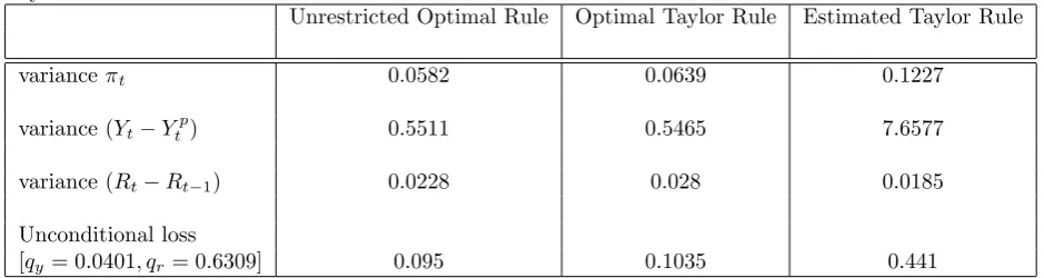
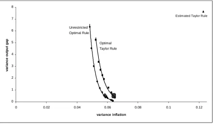
5. Implied Variances and Tylor Rules... 28
6. A note on the Lagrange Multipliers and the Timeless Perspective ... 31
7. Conclusion ... 34
References ... 35
Appendix ... 40
1
Introduction
Correct knowledge of the variables that are of main concern for monetary policy is an important
asset since knowing the alternative monetary policy targets and their relative importance with
respect to each other will have an e¤ect on the formation of private sector expectations. Given
the importance of these expectations and the role they play in stabilizing the economy, it is
desirable for monetary policy makers to provide the private agents with su¢ cient information
concerning the relative importance of each target variable. The value attached to a particular
target variable, for example the in‡ation target, by monetary authorities can be described by
the relative weight assigned to this target in the loss function that the Central Bank aims to
minimize over the in…nite horizon. The relative weights therefore generally re‡ect the preferences
of monetary policy makers with respect to the corresponding target variables.
In order to infer the monetary policy preferences, one could analyze empirical monetary policy
reaction functions and study the behaviour of monetary policy makers. This kind of approach,
however, has often been criticised (Svensson, 2002a, 2003 and Dennis, 2000, 2002, 2003, 2005 and
2006). The argument is based on the idea that, while an estimated reaction function gives a good
description of monetary policy behaviour, the intertemporal loss function is a more appropriate
measure of (changes in) monetary policy objectives. In the context of optimal monetary policy, a
reaction function is only a reduced form and results from a complex optimization problem of the
Central Bank. Hence the variables entering the reaction function mainly play a role in providing
monetary policy with information needed to achieve the policy objectives. These variables
are therefore not necessarily equal to the target variables that appear in the loss function and
cannot be attributed directly to the monetary policy objectives. In addition, the implied explicit
interest rate reaction function from the optimization problem under certain policy objectives will
typically contain more information by including the complete state vector, whereas a prespeci…ed
estimated reaction function is restricted to respond to only a subset of the state variables. A
more theoretical justi…cation for assuming a single representative monetary policy maker that
systematically optimizes an intertemporal loss function, as in Svensson (1999) and Woodford
(2003), is that this approach towards monetary policy will bring monetary policy behaviour in
line with the behaviour of private agents. Hence we adopt a general equilibrium framework
with rational and optimizing agents, where all structural equations result from optimal decisions
made by private agents as well as monetary policy makers. This framework would also make it
value of in‡ation (Dennis, 2004).
An extensive amount of studies in the literature has recently focused attention on the
estima-tion or calibraestima-tion of preferences of optimizing monetary policy authorities, which is analogous to
estimating the weights assigned to the target variables in the intertemporal optimization problem
of the Central Bank. Many of these estimation exercises in the context of forward-looking models
consider the case of discretionary monetary policy where optimization occurs every period and
private sector expectations are treated as constants, as in Dennis (2000, 2003), Söderström et al.
(2003) and Castelnuovo (2004) for the US economy and Lippi and Neri (2005) for the euro area
economy1. The case of full commitment as in Söderlind (1999) or commitment to a simple rule of
the kind adopted by Salemi (2001) for the US economy has, to our knowledge, not been applied
to the euro area economy. This is probably due to the time-inconsistency problem one has to
deal with under commitment. The aim of this paper is to study the case of monetary policy
that systematically minimizes an intertemporal quadratic loss function under full commitment
in a forward-looking model for the euro area. A commitment strategy, if credible, enables the
Central Bank to control the expectations of private agents and provides it with an additional
stabilization tool. We consider the Smets and Wouters (henceforth SW) (2003) model for the
euro area as the benchmark model, where we drop the estimated Taylor rule and replace it by
monetary policy that minimizes an intertemporal loss function under commitment subject to the
structural model of the economy. This enables us to estimate the preference parameters of the
monetary policy objective function jointly with the structural parameters of the model economy.
The estimations are performed using Bayesian methods, considering alternative forms of
mone-tary policy objective functions that di¤er in their assumptions about the number and type of the
target variables. We use the values of the preference parameters obtained from the estimations
to derive the optimal Taylor rule within the benchmark SW (2003) model and look to which
extent the optimized feedback coe¢ cients di¤er from the estimated coe¢ cients of the Taylor
rule in the original SW (2003) set up. In addition, we compare the results for the structural
parameters obtained from the modi…ed model with optimal monetary policy to the results of the
original SW (2003) model, assigning di¤erences to the alternative ways that monetary policy is
described. This comparison is based on the marginal likelihood values and impulse response
analysis. We make an attempt to overcome, empirically, the time-inconsistency problem that
comes along with optimization under commitment by considering an initialization period that is
1Dennis (2006) and Ozlale (2003) perform a similar exercise for the US in the context of the Rudebusch and
long enough to reduce the e¤ect of the initial values on the estimation results. This way, we are
able to implement the timeless perspective framework of Woodford (1999).
This paper is organized as follows. In the next part we outline the theoretical framework
adopted in this paper. We start from the SW (2003) model and describe the assumed structural
behaviour of the private agents in the economy, followed by the introduction of optimal monetary
policy, which leads to a set of Euler equations that can be estimated accordingly. In introducing
optimal monetary policy we consider two types of loss functions that appear to perform best
among a large set of alternative speci…cations. The …rst loss function includes in‡ation, the
model-consistent output gap and the interest rate di¤erential as target variables, whereas the
second loss function considers an additional wage in‡ation target. The third part explains the
methodology adopted and the data set used in the estimation procedure, followed by a discussion
of the results. We compare alternative models based on their marginal likelihood and discuss
the impulse responses obtained under the best performing model that is characterized by optimal
policy with respect to the benchmark impulse responses of SW (2003) in part four. In part …ve
we derive the unrestricted optimal commitment rule and the optimal coe¢ cients of the Taylor
rule, which we compare to the estimated Taylor rule of SW (2003). Accordingly, we refer to
the potential time-inconsistency problem due to our commitment framework and show how we
circumvent this issue by adopting the concept of timeless perspective policy of Woodford (1999)
in part six. Finally, part seven concludes.
2
Theoretical Framework
The structural behaviour of the euro area economy is assumed to be described by the model
developed by Smets and Wouters (2003). In this type of micro-founded framework private agents
base their individual decisions on optimizing behaviour. This results in aggregate structural
equations of which the parameters re‡ect deep preferences of the agents. However, instead of
capturing the behaviour of the monetary policy authorities by an empirical Taylor rule as is
done in the original set up of the SW (2003) model, we will assume that monetary policy is
performed optimally under commitment. This will ensure that monetary authorities behave
more consistently and in analogy with the private agents2. Moreover, this approach will allow
us to estimate the preferences of monetary policy makers over the target variables. Following
the arguments outlined in e.g. Svensson ( 2002a, 2003), Dennis (2000, 2003) and Lippi and Neri
(2005)3, estimating the policy preferences rather than the monetary policy reaction function
is more desirable since the latter is only a function of the former. Describing the behaviour
of monetary policy authorities in terms of their preferences yields therefore more and better
information about their incentives underlying their actions in response to economic developments
than estimated interest rate reaction functions. In the following we present a brief summary of
the linearized SW (2003) model for the euro area and introduce the optimizing monetary policy
authorities. The resulting model, that takes into account optimal monetary policy behaviour
under commitment, can accordingly be estimated with euro area data. Our main intention is to
compare these results to those obtained under the original SW (2003) speci…cation of the model.
2.1
The Smets and Wouters model for the Euro Area
The Dynamic Stochastic General Equilibrium (DSGE) framework presented in SW (2003) for the
euro area consists of a household sector that supplies a di¤erentiated type of labour, leading to
nominal rigidities in the labour markets. The goods markets are characterized by intermediate
and …nal goods producers. The former type of agents are monopolistically competitive and
produce a di¤erentiated type of intermediate goods, leading to nominal rigidities in the goods
markets. The latter type of agents operate in a perfectly competitive market and produce one
…nal good used for consumption and investment by the households.
Next to these nominal rigidities in the goods and labour markets, the model also features real
rigidities like habit formation, costs of adjustment in capital accumulation and variable capital
utilization. There are many similarities with the model presented in Christiano, Eichenbaum and
Evans (CEE) (2001). However, the SW (2003) model includes an additional number of structural
shocks, partial indexation to past in‡ation in the labour and the goods markets and is estimated
using (Bayesian) estimation methods. The linearized rational expectations equations that result
from private sector optimizing behaviour are summarized next, where the same notation as in
SW (2003) is adopted and where all variables are expressed as log deviations from their steady
state levels denoted by^, i.e. x^= log xx .4
The consumption Euler equation includes an external habit variable that leads to a
backward-3These studies assume, in contrast to our approach, that monetary policy is conducted under discretion. Lippi
and Neri (2005) also consider the euro area and incorporate the case of imperfect information in their estimation procedures.
4For a detailed description of the individual parameters and the optimizing behaviour of the agents that lead
looking component to capture habit persistence:
^
Ct=
h 1 +h
^
Ct 1+
1 1 +hEt
^
Ct+1 1 h (1 +h) c
^
Rt Et^t+1 +
1 h
(1 +h) c ^
"bt Et^" b
t+1 (1)
with^"btan AR(1) preference shock to the discount rate with an i.i.d. normal error term. Nominal wages are set by households according to a Calvo (1983) type of scheme. Households that cannot
reoptimize will adjust their nominal wages partially to past in‡ation with a degree0 w 1, leading to the following real wage equation:
^
wt =
1 + Et
^
wt+1+
1 1 +
^
wt 1+
1 + Et
^ t+1
1 + w
1 +
^
t+ w 1 +
^ t 1
1 1 +
(1 w) (1 w) ( w+(1+ w) L
w ) w
^
wt L
^
Lt c 1 h(
^
Ct h ^
Ct 1) ^"
L
t wt (2)
where w is a constant in w;t = w+ wt with w;t a shock to the wage mark-up assumed to
be i.i.d. normal around the constant term and ^"Lta shock to labour supply assumed to follow an AR(1) process with an i.i.d. normal error term. The investment equation, characterized by
adjustment costs depending on the size of investments, is described as follows:
^
It= 1 1 +
^
It 1+
1 + Et
^
It+1+
' 1 +
^
Qt+
Et^" I t+1
^
"It
1 + (3)
with ^"It an AR(1) shock to investment costs with an i.i.d. normal error term. The real value of capital is represented by:
^
Qt= ( ^
Rt ^t+1) +
1
1 +rk
Et ^
Qt+1+ r k
1 +rk
Et^r k t+1+
Q
t (4)
with Qt an i.i.d. normal shock that captures changes in the external …nance premium due to
informational frictions. The capital accumulation equation ful…lls5:
^
Kt= (1 ) ^
Kt 1+
^
It (5)
As in the case of wage setting by households, the intermediate goods producers set their prices
in line with Calvo (1983). Firms that are not able to reoptimize adjust their price partially to
past in‡ation with a degree0 p 1, leading to the following New-Keynesian Phillips curve:
^ t =
1 + p
Et^t+1+ p
1 + p
^
t 1 (6)
+ 1
1 + p
1 p 1 p
p
^
rkt+ (1 ) ^
wt ^" a t + pt
5Note that we correct for a typo in SW (2003) by replacing lagged investment by its current value. In
where^"at is an AR(1) productivity shock with i.i.d. normal error term. The …nal term in square
brackets represents the real marginal costs augmented with an i.i.d. (cost-push) shock pt to the mark-up in the goods market, i.e. p;t = p+ pt. The labour demand equation for a given
capital stock is given by:
^
Lt= w^t+ (1 + )^r k t+
^
Kt 1 (7)
Finally, the goods market equilibrium condition is represented by the following expression where
total output equals total demand for output by households and the government (…rst line) and
total supply of output by the …rms (second line):
^
Yt = cy ^
Ct+gy"Gt + ky ^
It+r k
ky ^r k
t (8)
= (^"at + K^t+ ^r k
t+ (1 ) ^
Lt)
where"G
t is an AR(1) government spending shock with i.i.d. normal error term.
In order to complete the model we introduce optimizing monetary policy authorities, discussed
in the next section, which distinguishes our model from the original SW (2003) speci…cation where
monetary policy is described by a generalized empirical Taylor rule of the following type6:
^
Rt = ^
Rt 1+ (1 ) t+r (^t 1 t) +ry( ^
Yt 1
^
Ytp1) (9)
+r (^t ^t 1) +r y(( ^
Yt ^
Ytp) (Y^t 1
^
Y
p
t 1)) + Rt
where is the monetary authorities’smoothing parameter and R
t an i.i.d. monetary policy shock.
In addition to the one-period di¤erence in in‡ation and the output gap, a gradual response to
lagged in‡ation and lagged output gap is assumed. Since the main di¤erence between the two
models is the way monetary policy is described, i.e. optimizing vs. empirical reaction function,
we will be able to attribute di¤erences in estimation results under both models to the speci…c
assumptions made about monetary policy behaviour7.
2.2
Optimal Monetary Policy
Monetary policy authorities are assumed to minimize a discounted intertemporal quadratic loss
function of the following type:
Et 1
X
i=0
i
[yt0+iW yt+i], 0< <1 (10)
6Note that we correct a typo in SW (2003) in the …rst line of the rule where the lag of the output gap appears
instead of the current output gap.
7Note that we also do not include the in‡ation ob jective shock,
t, in the model with optimal policy. This
with the discount factor andEtthe expectations operator conditional on information available
at time t. This type of quadratic loss function is commonly adopted in the literature, as in
Rudebusch and Svensson (1998), Giannoni and Woodford (2003), Söderlind (1999) and Dennis
(2005). The vectoryt= [x0t u0t]0 contains then 1endogenous variables and AR(1) exogenous
variables in the model included in xt and the p 1 vector of control variables included in ut.
Since we assume only one control variable, i.e. the interest rate, ut is in our case a scalar with
ut = ^
Rt. W is a time-invariant symmetric, positive semi-de…nite matrix of policy weights
which re‡ect the monetary policy preferences of the Central Bank over the target variables. An
alternative and theoretically more justi…able approach towards monetary policy would be to
derive the approximated welfare based loss function, where the target variables and their weights
in the loss function are determined by the utility of the households. However, this is not an easy
task given the presence of variable capital utilization and investment dynamics in the model.
Therefore we will assume a quadratic ad hoc loss function in this study8.
We follow standard practice in the literature9 in assuming that the one-period ad hoc loss
function for (10) re‡ects the fact that monetary policy targets in‡ation, a measure of the output
gap and a smoothing component for the policy instrument which is described by the interest
rate:
Lt= ^t
2
+qy( ^
Yt ^
Ytp)2+qr( ^
Rt ^
Rt 1)2 (11)
As explained in the next part, the dataset used in the estimation procedure contains series
on (detrended) in‡ation considered in deviation from its sample mean. Since we normalize
the in‡ation target in (11) to zero, this implies that monetary policy aims to stabilize in‡ation
around the sample mean. Hence the sample mean is considered to be the in‡ation target,
which is a known constant10. The inclusion of the termR^t ^
Rt 1 in the loss function, as in
Rudebusch and Svensson (1998) and Giannoni and Woodford (2003), can be justi…ed by concerns
about …nancial stability or in order to take into account the observed inertial behaviour in the
policy instrument, which suggests a gradualist monetary policy approach11. The output gap
8See Onatski and Williams (2004) for an exercise on welfare based approximation to the loss function in the
SW (2003) model and Levin et al. (2005) for a similar study.
9See e.g. Rudebusch and Svensson (1998), Giannoni and Woodford (2003), Dennis (2003), Söderström et al.
(2003), Lippi and Neri (2005) and Castelnuovo (2004).
1 0One could criticise this approach and alternatively consider the in‡ation target as an additional parameter
to be estimated. We would like to consider this apporach as an extension to this paper in the near future.
Conditions under which the in‡ation target can be identi…ed and estimated are provided by Dennis (2003,2004). 1 1In our estimation exercises performed in the next part, we replace this …nal term by the interest rate level, i.e.
^ R 2
t, a case studied by e.g. Giannoni and Woodford (2002), Woodford (2003) and Onatski and Williams (2004).
considered here is the one implied by the model, i.e. the deviation of output from its natural
level, the latter being the level of the output in total absence of nominal rigidities and the
three i.i.d. cost-push shocks ( Qt ; pt; wt)12. As is done in most applications in the literature, the weight assigned to in‡ation in the above loss function is normalized to one13. Hence the
weights corresponding to the output gap and the interest rate smoothing component, i.e. qy
andqr, respectively, are to be interpreted as relative weights with respect to the in‡ation target
variable. We will estimate the preferences of monetary policy re‡ected by these parameters
along with the structural parameters of the economy, which will provide us with values for the
weights in the loss function over the estimation period. These values will be accordingly used
in the optimal monetary policy evaluation exercises performed in part …ve.
Since the structural model of the economy outlined above is characterized by nominal wage
rigidities, it is appealing from a theoretical point of view to investigate also the case where
monetary policy is concerned about stabilizing nominal wage in‡ation in addition to the target
variables in (11). A case for a nominal wage in‡ation target is provided by Erceg et al. (1998,
1999) where, as in Kollmann (1997) and Woodford (2003), a dynamic general equilibrium model
featuring staggered wage and price setting is developed and where the authors show that rigidities
in these both markets at the same time make the Pareto optimal equilibrium unattainable for
monetary policy. Hence there is a tradeo¤ between price, wage and output gap stabilization.
Moreover, Erceg et al. (1999) derive a social welfare function under the circumstances of nominal
wage and price rigidities and show that there are high welfare costs attached to targeting price
in‡ation only and ignoring wage in‡ation stabilization. In the welfare based loss function derived
for the SW (2003) model by Onatski and Williams (2004), a term for wage in‡ation is also
included14. Therefore, we will analyze also the following alternative speci…cation of the loss
function, where monetary policy aims to target nominal wage in‡ation as well:
Lt= ^t
2
+qy( ^
Yt ^
Ytp)2+qr( ^
Rt ^
Rt 1)2+qw( ^
Wt ^
Wt 1+ ^t)2 (12)
1 2Although it is more common in empirical applications that deviations of output from a linear trend are
used as an approximation to the output gap, we prefer to adopt the theoretical concept of the output gap. To
support this choice, we experiment with alternative de…nitions of the output gap in the next part which yield less favourable results in terms of the marginal likelihood.
1 3Examples can be found in Rotemberg and Woodford (1998), Rudebusch and Svensson (1998), Dennis (2003)
and Woodford (2003).
1 4In addition, Onatski and Williams (2004) include a positive weight on the capital stock and the covariance
between in‡ation and wages. This results in an approximated loss function of the typeLt= ^t
2
+ 0:21K2
t 1
0:51^t t^1+ 0:24( ^
Wt+ ^t)(
^
Wt
^
Wt 1). We consider this speci…cation also in the next part, where the
The speci…cation of the one period loss function in (11) can be considered as a special case of (12)
whereqwis set to0. We will estimate the model under both speci…cations of the loss function,
by treating the case under each one of the two speci…cations as a separate model. Therefore, we
will refer to the case whereqw= 0, i.e. period loss function (11), as modelM1and consider the
case where nominal wage in‡ation is an additional target variable as modelM2. We then use
the corresponding marginal likelihood values in order to rank the two models and assess to which
extent monetary policy has been concerned about nominal wage in‡ation stabilization over the
sample period15.
The Central Bank minimizes the intertemporal loss function (10), the one-period loss function
of which is given by either (11) or (12), under commitment subject to the structual equations of
the economy (1) - (8) augmented by their ‡exible price versions, written and represented by the
following second order form:
Axt=BEtxt+1+F xt 1+Gut+Dzt, zt iid[0; zz] (13)
with zt ann 1 vector of stochastic innovations to the variables inxt, having mean zero and
variance-covariance matrix zz.
Under commitment the central bank optimizes only once in the initial period t0, ignoring
past promises but tying its hands by promising att0to follow the resulting policy rule forever16.
The resulting equilibrium is not time consistent and past commitments will be respected only in
the future periods to come aftert0, therefore making policy history dependent only from t0 on.
This is re‡ected by the presence of the Lagrange multipliers in the optimal reaction function17.
We follow the optimization routine for commitment suggested by Dennis (2005) where, in
contrast to e.g. Söderlind (1999), no classi…cation of the variables in a predetermined and a
non-predetermined block is needed. We further adopt the de…nition of rational expectations as
proposed by Sims (2002), i.e.
Etxt+1+ xt+1=xt+1 (14)
1 5We admit that in this study we make the strong assumption that the monetary policy regime has been
unchanged in the euro area throughout the sample period. This might be doubtful given the separate monetary policy strategies adopted in the individual countries before the introduction of the Euro. However, the transition period towards the Euro and the restrictions imposed by the Maastricht treaty justify our assumption that the policy regimes were more likely to have been in line rather than divergent.
1 6Past promises are ignored by setting initial values of the Lagrange multipliers equal to zero.
1 7However, we will make an attempt to overcome this time-inconsistency problem in our estimation procedure,
and partition the matrix of weightsW in (10) as follows:
Et 1
X
i=0
i[x0
t+iQxt+i+u0t+i ut+i]; 0< <1 (15)
where we express the loss function in terms of the variablesxtandut. Accordingly, we obtain
the Euler equations of the monetary policy optimization problem, which can be represented in
the following second order form:
A1 t=B1 Et t+1+C1 t 1+D1 zt (16)
with:
A1 =
2
4 Q 0 A
0
0 G0
A G 0
3
5 B1 = 2
4 0 0 F
0
0 0 0
B 0 0
3
5 (17)
C1 =
2 4 0 0
1B0
0 0 0
F 0 0
3
5 D1 = 2 4 00
D 3
5 and t=
2 4 xutt
t
3 5= yt
t
and the …nal term in t, t, the vector of Lagrange multipliers. It is clear from the system
of Euler equations (17) that the economy’s law of motion (13), which reappears in the last line
in (17), is augmented by the set of …rst order conditions with respect to xt and ut, through
which the (leads and lags of the) Lagrange multipliers tenter into the system and the matrices
A1 ; B1 ; C1 have dimension (2n+p) (2n+p)18. In the next part, we will estimate the
Euler equations resulting from the optimization procedure outlined above, i.e. the system (16),
by applying Bayesian estimation techniques.
3
Estimation
In this part we discuss the dataset used and the methodology followed in estimating the system
(16), which yields estimates of the structural parameters resulting from optimizing private agents
and policy preferences of optimizing monetary policy authorities. Next, we present the results
under M1 and M2 and compare them to each other and to the estimates obtained from the
benchmark model in SW (2003).
3.1
Data
We use the same dataset as the one used by SW (2003) for the euro area, i.e. constructed
by Fagan, Henry and Mestre (2001). The dataset contains observed series on real GDP, real
1 8A more detailed illustration of the state space expansion and the inclsuion of the leads and lags of the
consumption, real investment, GDP de‡ator, real wages, employment and the nominal interest
rate. The series range over the period 1980:2 - 1999:4, preceded by an initialization period of
40 quarters in order to initialize the estimates. The reason why we opt to end the observation
period in the last quarter of 1999 is for comparison of the estimation results to those obtained
under the original speci…cation of the model in SW (2003), where monetary policy is assumed
to follow a generalized Taylor rule. Furthermore, as in SW (2003), all variables are considered
in deviations from their sample means. In‡ation and nominal interest rates are detrended by
the in‡ation trend, whereas the remaining variables in the dataset are detrended separately by a
linear trend. As explained in SW (2003), we introduce an additional equation for employment
to correct for the use of data on employment instead of the unobserved data on aggregate hours
worked in the euro area:
^
Et ^
Et 1=
^
Et+1
^
Et+
(1 e) (1 e) e
^
Lt ^
Et (18)
We further introduce an i.i.d. measurement error R
t to take account for mismeasurement in the
observed series of the nominal interest rate (R^
obs
t ), leading to the following relation between the
observed and the non-observed policy instrument rate19:
^
R
obs t =
^
R
nobs
t + Rt (19)
As opposed to SW (2003), the two monetary policy shocks that appear in the generalized Taylor
rule, i.e. a shock to the in‡ation objective and an interest rate shock, are absent from the models
M1 and M220. As in SW (2003), identi…cation is obtained through the assumption that all
shocks are uncorrelated, that the three cost-push shocks together with the measurement error
follow a white noise process and that the remaining shocks related to preferences and technology
are AR(1). In order to compare our results to those obtained by SW (2003), we use the same
prior speci…cations for those parameters that correspond to the parameters in the original model.
Therefore, we …x the following parameters: the discount factor is set equal to 0:99, implying
an annual real interest rate of4 percent. The annual depreciation rate on capital is assumed to
be10 percent, i.e. = 0:025. The income share of labour in total output is assumed to be0:7
in the steady state, i.e. = 0:3. The share of consumption and investment in total output is
0:6and0:22in the steady state, respectively. Finally, w is calibrated to be0:5, for reasons of
1 9This measurement error could be compared to a monetary policy shock, since it takes account for the observed
di¤erence between the actual interest rate and the systematic movements in the interest rate as implied by the
model. Although the interpretation of this measurement error, in contrast to the monetary policy shock in the
original SW (2003) model, is not a structural one.
identi…cation. In the next section we outline the methodology adopted in the estimation of the
remaining parameters.
3.2
Methodology
We apply Bayesian estimation techniques in order to estimate the parameters of the alternative
models21. After solving for the linear rational expectations solution of the model in (16), we
derive the following state transition equation:
t= Y t 1+ zzt (20)
and the measurement equation that links the state variables tlinearly to the vector of
observ-ables t,
t= Y t (21)
We use the Kalman …lter to calculate the likelihood function of the observables recursively,
start-ing from initial values of the state vector 0 = 0and the unconditional variances22. Next, the
posterior density distribution is derived by combining the prior distribution with the likelihood
function obtained from the previous step. We proceed until the parameters that maximize the
posterior distribution are found, i.e. until convergence around the mode is achieved. After
max-imizing the posterior mode, we use the Metropolis-Hastings algorithm to generate draws from
the posterior distribution in order to approximate the moments of the distribution, calculate the
modi…ed harmonic mean and construct the Bayesian impulse responses23. In discussing the
es-timation results, however, we will focus on the maximized posterior mode and the Hessian-based
standard errors.
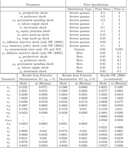
In Table 1 the …rst three columns show the details of the prior distributions for the shock
processes, i.e. the standard errors of all nine shocks and the AR(1) coe¢ cients of the …ve
preference shocks. The type of the prior distributions, the prior means and the prior standard
errors are identical to the assumptions made in SW (2003) and are kept constant throughout
the estimation processes for both modelsM1andM2. All variances of the shocks are assumed
to have an inverted gamma distribution with2degrees of freedom, except for the measurement
error which we assume to be gamma distributed with a prior mean of0:05and standard error of
2 1For a detailed discussion in favour of Bayesian estimation of DSGE models, we refer to SW (2003-2005),
Schorfheide (2006) and An and Schorfheide (2006).
2 2As discussed next, we experiment also with initial values at nonzero for certain lagrange multipliers in order
to incorporate the concept of optimal policy under the "timeless perspective".
2 3All estimations are performed using Michel Juillard’s software dynare, which can be downloaded from the
0:025. The …ve AR(1) coe¢ cients are assumed to have a beta distribution with a prior mean of
0:85and a strict prior standard error of0:1 in order to distinguish the persistent shocks clearly
from the i.i.d. shocks. Table 1 also reports the results obtained from the posterior maximization,
i.e. the posterior mode and the (Hessian-based) standard errors for the models M1, M2 and
the original SW (2003) model. These results are discussed and compared in the next section.
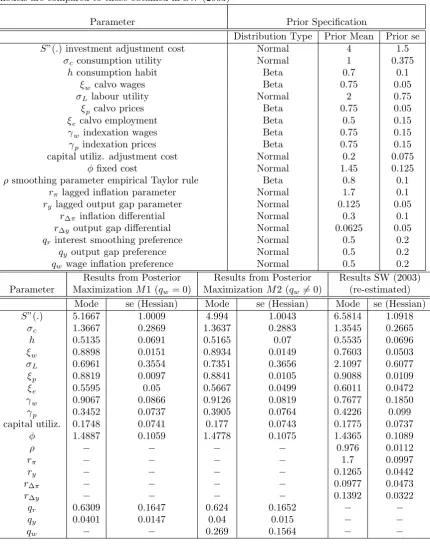
The results for the structural parameters are reported in Table 2, together with the SW (2003)
results. The prior speci…cations and the estimates of the monetary policy preference parameters,
i.e. the weights assigned to the target variablesqy,qrandqw are reported in the bottom part of
the table. These parameters are assumed to be normally distributed with0:5 prior mean and
0:2prior standard error.
3.3
Results
As mentioned before, we report and discuss only the estimation results obtained forM1andM2
because under these two types of the loss function highest marginal likelihoods were obtained24.
We also re-estimate the SW (2003) model25 which will serve as a benchmark for the results
obtained under modelsM1 andM2with optimal monetary policy.
3.3.1 Structural Shocks and Private Sector Parameters
Turning to the results concerning the structural shocks reported in Table 1, the estimated
pa-rameters and their corresponding standard errors under our speci…cation M1 of the model are
similar to those underM2. A few remarks are worth making when we compare the results under
both models to our estimates of the benchmark SW (2003) model. The estimates of the labour
supply shock land the equity premium shock Q are considerably lower under the modelsM1
and M2, compared to SW (2003). In addition, the labour supply shock turns out to be more
persistent underM1 andM2than under SW (2003). A higher persistence is also estimated for
the productivity shock. The wage mark-up shock W is higher underM1andM2than the SW
(2003) estimate.
Comparing the SW (2003) estimates for the structural parameters to these obtained under
M1 and M2, which are reported in Table 2, yields the following conclusions. The investment
2 4In our experiments we consider alternative loss functions where we replace the interest rate smoothing term
by the interest rate level, or the output gap by the di¤erences in output. We also studied the case where we
used simply output deviations from a linear trend instead of the model-consistent output gap. We examined loss functions including a di¤erence in the output gap, a di¤erence in the in‡ation rate or of the welfare approximated type presented by Onatski and Williams (2004) as well. None of these cases, however, could yield better outcomes in terms of their corresponding marginal likelihoods.
2 5These results appear to be very similar to those reported in the original SW (2003). However, mainly due
Table 1: Prior speci…cations and estimates of the shocks, with the standard errors followed by the AR(1) coe¢ cients. Both speci…cations are compared to the results obtained in SW (2003)
Parameter Prior Speci…cation
Distribution Type Prior Mean Prior se
a productivity shock Inverse gamma 0:4 2 b preference shock Inverse gamma 0:2 2 G government spending shock Inverse gamma 0:3 2 l labour supply shock Inverse gamma 1 2 I investment shock Inverse gamma 0:1 2 Q equity premium shock Inverse gamma 0:4 2 P price mark-up shock Inverse gamma 0:15 2 W wage mark-up shock Inverse gamma 0:25 2
in‡ation objective shock (only SW (2003)) Inverse gamma 0:02 2 M P monetary policy shock (only SW (2003)) Inverse gamma 0:1 2
R measurement error (onlyM1 andM2) Gamma 0:05 0:025
in‡ation objective shock (only SW (2003)) Beta 0:85 0:1
a productivity shock Beta 0:85 0:1 b preference shock Beta 0:85 0:1 G government spending shock Beta 0:85 0:1 L labour supply shock Beta 0:85 0:1 I investment shock Beta 0:85 0:1
Results from Posterior Results from Posterior Results SW (2003) Parameter MaximizationM1(qw= 0) MaximizationM2(qw6= 0) (re-estimated)
Mode se (Hessian) Mode se (Hessian) Mode se (Hessian)
a 0:5252 0:0771 0:5366 0:0806 0:6051 0:1097 b 0:2031 0:0475 0:1909 0:0465 0:2577 0:0805 G 0:3236 0:0256 0:3234 0:0255 0:3225 0:0254 l 1:8033 0:3533 1:8406 0:3629 4:1880 1:4832 I 0:0498 0:0159 0:0523 0:0174 0:0639 0:0177 Q 0:4907 0:0602 0:4862 0:0615 0:5984 0:0594 P 0:1595 0:0152 0:1578 0:015 0:1576 0:015 W 0:3423 0:0289 0:3428 0:0292 0:2881 0:0266
0:0092 0:0038
M P 0:0562 0:0252
R 0:0354 0:0082 0:0351 0:0085
0:9221 0:0863
Table 2: Prior speci…cations and estimates of the structural parameters. The results for both models are compared to those obtained in SW (2003)
Parameter Prior Speci…cation
Distribution Type Prior Mean Prior se
S"(:)investment adjustment cost Normal 4 1:5
c consumption utility Normal 1 0:375
hconsumption habit Beta 0:7 0:1
w calvo wages Beta 0:75 0:05
L labour utility Normal 2 0:75
p calvo prices Beta 0:75 0:05 e calvo employment Beta 0:5 0:15 w indexation wages Beta 0:75 0:15 p indexation prices Beta 0:75 0:15
capital utiliz. adjustment cost Normal 0:2 0:075
…xed cost Normal 1:45 0:125
smoothing parameter empirical Taylor rule Beta 0:8 0:1 r lagged in‡ation parameter Normal 1:7 0:1 ry lagged output gap parameter Normal 0:125 0:05
r in‡ation di¤erential Normal 0:3 0:1 r y output gap di¤erential Normal 0:0625 0:05
qr interest smoothing preference Normal 0:5 0:2
qy output gap preference Normal 0:5 0:2
qw wage in‡ation preference Normal 0:5 0:2
Results from Posterior Results from Posterior Results SW (2003) Parameter MaximizationM1(qw= 0) MaximizationM2 (qw6= 0) (re-estimated)
Mode se (Hessian) Mode se (Hessian) Mode se (Hessian)
S"(:) 5:1667 1:0009 4:994 1:0043 6:5814 1:0918 c 1:3667 0:2869 1:3637 0:2883 1:3545 0:2665
h 0:5135 0:0691 0:5165 0:07 0:5535 0:0696
w 0:8898 0:0151 0:8934 0:0149 0:7603 0:0503 L 0:6961 0:3554 0:7351 0:3656 2:1097 0:6077 p 0:8819 0:0097 0:8841 0:0105 0:9088 0:0109 e 0:5595 0:05 0:5667 0:0499 0:6011 0:0472 w 0:9067 0:0866 0:9126 0:0819 0:7677 0:1850 p 0:3452 0:0737 0:3905 0:0764 0:4226 0:099
capital utiliz. 0:1748 0:0741 0:177 0:0743 0:1775 0:0737
1:4887 0:1059 1:4778 0:1075 1:4365 0:1089
0:976 0:0112
r 1:7 0:0997
ry 0:1265 0:0442
r 0:0977 0:0473
r y 0:1392 0:0322
qr 0:6309 0:1647 0:624 0:1652
qy 0:0401 0:0147 0:04 0:015
adjustment cost parameter is estimated to be lower ( 5:1667 and4:994) than the baseline
esti-mated value of6:5814, whereas the standard errors are similar. This suggests a higher elasticity
of investment with respect to an increase in the current price of installed capital of 1 percent
under M1 and M2. A strikingly higher value is obtained under M1 and M2 for the Calvo
wage parameter w than in the baseline case (0:8898and0:8934vs. 0:7603). The same
conclu-sion holds for the wage indexation parameter w with 0:9067 and0:9126 vs. 0:7677. Hence a signi…cantly higher wage stickiness and wage indexation is present whenever monetary policy is
assumed to behave optimally as is the case underM1and M2, suggesting an average duration
of wage contracts of slightly more than two years. The reverse conclusion can be drawn from
estimates for the Calvo price p and the price indexation parameter p. These parameters are signi…cantly lower under the models characterized by optimizing monetary policy authorities,
yielding 0:8819 and0:8841for p vs. the SW (2003) estimate of 0:9088and 0:3452 and0:3905
for p vs. 0:4226. The former suggests a lower degree of price stickiness in the goods markets under M1 andM2compared to SW (2003) with an average duration of price contracts of two
years, which is very close to the average duration of the wage contracts, implying a similar
de-gree of stickiness in wages and prices underM1 andM2. The estimates of p imply that price indexation is lower underM1andM2, and in line with the …ndings of Gali et al. (2001) for the
euro area where a low degree of backward-looking behaviour in the goods market is estimated.
Finally, the estimate of the labour utility parameter L is considerably lower under the models
M1 andM2(0:6961and0:7351) than under SW (2003) (2:1097)26.
3.3.2 Monetary Policy Preference Parameters
Table 2 also shows the parameter estimates of our main interest, i.e. the monetary policy
preferences in the two modelsM1 and M227. The estimates of the policy preferences for the
interest rate smoothing target qr and the output gap target qy are very similar for the two
alternative speci…cationsM1andM2. In both cases the preference for interest rate smoothing
is estimated to be higher (0:6309 and 0:624) than the preference for output gap stabilization
(0:0401 and 0:04), while overall the main concern is still the in‡ation target whose weight is
2 6Note that, as was the case in the original SW (2003), our estimates of this parameter did not appear to be
robust across speci…cations either...
2 7Since in‡ation and the interest rates, both target variables, are measured on a quartely basis and the literature
occasionally considers target variables on a yearly frequency, the weights obtained from the estimates have to be adjusted in order to make the results comparable to those in the literature which base their results on yearly
data. Therefore, from the viewpoint of these studies, the weight assigned to the output gapqy is not as small
as it seems at …rst sight. Taking this into account boils down to multiplyingqyby a factor of 16 and converting
the in‡ation and the interest rate in the model to a yearly frequency . Hence, the values forqywould become
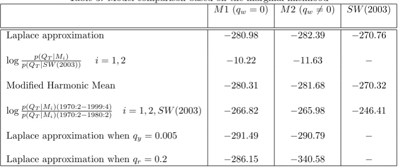
Table 3: Model comparison based on the marginal likelihood
M1 (qw= 0) M2 (qw6= 0) SW(2003)
Laplace approximation 280:98 282:39 270:76
log p(QTjMi)
p(QTjSW(2003)) i= 1;2 10:22 11:63
Modi…ed Harmonic Mean 280:31 281:68 270:32
logp(QTjMi)(1970:2 1999:4)
p(QTjMi)(1970:2 1980:2) i= 1;2; SW(2003) 266:82 265:98 246:41
Laplace approximation whenqy = 0:005 291:49 290:79
Laplace approximation whenqr= 0:2 286:15 340:58
normalized to one. However, when we investigate the importance of the output gap as a target
variable by calculating the marginal likelihood cost of decreasing the weight qy from 0:0401 to
e.g. 0:005, the importance attached to the output gap appears to be higher than the estimates
suggest28.
As the …rst line in Table 3 shows, a value ofqy = 0:0401is accomodated by a higher marginal
likelihood than whenever the weight is decreased to 0:005 (second last line in Table 3)29. In
addition, the impulse response dynamics of the target variables, which are shown in …gures 1
and 2 for the productivity shock and the price mark-up shock, respectively30, is di¤erent when
we set qy = 0:005 (purple line) compared to the case where the weight is only slightly higher,
i.e. 0:0401as inM1 (dark line). In both …gures, there is mainly a remarkable di¤erence in the
dynamics of the output gap, which takes a longer time to return to equilibrium whenqy= 0:005.
2 8It should also be noted that, in order to evaluate the relative importance of the components in the loss
function, their corresponding weights should be combined with the realtive volatility of the related variables. Hence the weights per se are not su¢ cient to evaluate the importance of the alternative target variables, due to the fact that the output gap concept we use in this study is a theoretical one.
2 9The marginal likelihood keeps deteriorating with the decrease inq
y. For example, settingqyequal to0:01
brings only a slight deterioration in the marginal likelihood ( 281:95). Whenqy= 0:001the marginal likelihood
already drops to 335:96and to 499:24whenqy= 0.
Figure 1. Impulse response to productivity shock whenqy= 0:005 vs. qy= 0:0401(M1)
Figure 2. Impulse response to price mark-up shock when qy = 0:005vs. qy= 0:0401(M1)
When we decrease the weight assigned to the interest rate smoothing target (i.e. qr) to a
value of 0:2, the marginal likelihood also deteriorates as is shown in the last line of Table 3,
although this worsening is smaller than in the case where we lower the weight on the output
gap. Likewise, the impulse responses of the target variables to a productivity shock and a price
mark-up shock shown in …gures 3 and 4, respectively, do not change a lot whenqr= 0:2 (purple
line) compared to the case where qr = 0:6309as in M1 (dark line). Overall, the output gap
[image:22.595.182.411.343.531.2]deterioration in the marginal likelihood is worse and the dynamics of the target variables di¤er
to a greater extent when models are re-estimated under the assumption that qy = 0:005 than
whenqr= 0:2. Therefore, although the weight on the output gap is estimated to be small, the
statement that the output gap could be ignored in the loss function would be too strong given
[image:23.595.181.411.204.387.2]the high e¤ect a decrease inqy has on the marginal likelihood and the impulse responses.
Figure 3. Impulse response to productivity shock whenqr= 0:2vs. qr= 0:6309(M1)
Figure 4. Impulse response to price mark-up shock whenqr= 0:2 vs. qr= 0:6309(M1)
In general, however, estimates of a small role for the output gap seem to …nd support in the
[image:23.595.182.411.437.622.2]although they use a di¤erent output gap concept than the one in this study31 and assume that
monetary policy is conducted under discretion, which requires some caution in comparing the
results. Dennis (2003) likewise …nds an ignorable weight for the output gap for the US under
discretionary monetary policy, which is in analogy with Lippi and Neri (2005)32. Söderlind
(1999), who also considers the case of commitment in estimating the policy preference parameters
and therefore provides a more appropriate comparison to our results, estimates a relatively high
value forqyin the framework of a standard loss function similar to (11). However, it is important
to keep in mind the fact that our output gap concept di¤ers from the one used in the other studies,
which makes direct comparison of the results a bit troublesome. While Svensson (1999, 2002b)
argues for a case of gradual monetary policy where some weight should be given to stabilizing
the output gap, and therefore requires a less activist policy, …ndings in the literature mentioned
above for qy generally do not support this concept of ‡exible in‡ation targeting. On the other
hand, our experiments with the marginal likelihood costs and impulse responses do imply that
somehow monetary policy has considered the output gap as an important target variable.
Lippi and Neri (2005) and Dennis (2003) estimate a weight on the interest rate smoothing
component that is higher than the weight on the in‡ation target, indicating a higher importance
attached to smoothing than to in‡ation33. This is not the case in our study. Although our
estimates of qr show that interest rate smoothing is a relatively important target, in‡ation
remains the main policy goal. From an economic point of view, this …nding is plausible and in
line with the statements that in‡ation should be the main target variable in monetary policy’s
objective function. Moreover, Castelnuovo (2004) …nds through a calibration exercise in the
framework of discretionary monetary policy, a value for the interest rate smoothing weight close
to ours whenever forward-looking agents are added to the model. When agents are assumed to
be backward-looking only, this weight increases considerably up to a point where interest rate
smoothing becomes twice as important as the in‡ation target. This leads Castelnuovo (2004)
to conclude that …nding an economically di¢ cult justi…able high value for qr is probably due
to model misspeci…cation by the omission of factors like forward-looking behaviour. Since the
model we consider includes forward-looking agents, our values of0:6309and0:624forqr are not
3 1Lippi and Neri (2005) describe the output gap as the deviation of output from a linear trend. On the
contrary, we assume that the output gap is the deviation of output from the natural output level in the absence of nominal rigidities and the three i.i.d. cost-push shocks.
3 2Söderström et al. (2003) show in their calibration exercise under discretion analogously a low concern for
output gap stabilization based on US data. See also Favero and Rovelli (2003) and Salemi (2001), who considers the case of commitment to an optimal Taylor rule, for …ndings of a relatively low weight on output gap stabilization.
3 3Söderström et al. (2003) show in their calibration exercise under discretion analogously a high importance
surprising34. An intuitive explanation for this moderating e¤ect of the presence of
forward-looking agents on the estimated weight assigned to the interest rate smoothing component in
the loss function can be given as follows35. Whenever (rational) agents are forward-looking,
their expectations will play a key role in the stabilization process of monetary policy and the
law of motion of the target variables. Thus current in‡ation and output are determined by
past expectations, and current expectations will determine future in‡ation and output. If the
economy is hit by a shock in the current period, requiring a change in the policy instrument rate
in order to stabilize the target variables, expectations will adjust accordingly and since agents
are rational they will take into account the fact that interest rate smoothing is a target variable
as well. Therefore a slow and persistent move in the interest rates is anticipated. Hence
expectations will have a stabilizing e¤ect on current in‡ation and output gap, which in turn
results in a slow and inertial behaviour in the interest rates. If agents were assumed to be
backward-looking, like in the case of Dennis (2006) and Ozlale (2003), this inertial behaviour in
the interest rates could be only taken into account by the assumption that smoothing receives a
high weight in the loss function of the central bank. If agents on the other hand are
forward-looking, interest rate inertia is attributed to the stabilizing e¤ect of expectations, which results in
lower concern for the interest rate smoothing target. In addition to this explanation, we would
also like to point out that the commitment framework assumed in this study enforces this history
dependence more than would be the case if monetary policy were assumed to optimize under
discretion like in most studies previously mentioned. This suggests that if we would perform
a similar exercise under discretionary monetary policy, the estimated values for qr would be
probably higher. This would be an interesting extension and a topic for future research. Our
estimates ofqrdo not seem to support the argument of Svensson (2002b, 2003), that an interest
rate stabilization or smoothing component should not enter the loss function at all, since the
values obtained for the smoothing target are signi…cantly higher than zero. However, as we
showed previously in this part, decreasing the value of qr does not lead to a very high loss in
terms of marginal likelihood, with a small change in the impulse responses compared to the case
where this parameter is freely estimated as is done inM1 andM2.
When nominal wage in‡ation is introduced in the loss function of monetary policy, as in the
3 4In order to assess this positive link between the degree of backward-lookingness and the estimates of the
preference for interest rate smoothing in our model, we look at the correlation between the series on the in‡ation
indexation parameter pand the interest rate smoothing preference parameterqrobtained from the markov chain
monte carlo draws. Based on these draws, we detect a positive correlation of around 0.3, which is in line with
the view of Castelnuouvo (2004).
3 5Castelnuovo (2004) provides a detailed explanation on this issue and quanti…es the role played by
case ofM2, this additional target receives a weight of0:269, which suggests a lower importance
attached to wage in‡ation stabilization with respect to the in‡ation target. However, on the
basis of comparison of marginal likelihoods in Table 3, theM1 speci…cation of the model where
qw = 0 is preferred over M2. Hence we can conclude that monetary policy is not concerned
about stabilizing nominal wage in‡ation and that in‡ation, interest rate smoothing and output
gap stabilization are its only targets.
Finally, we plot the prior and the posterior distributions of the parameters for modelM1 in
…gures A1-A3, which can be found in the Appendix. We apply the Metropolis-Hastings sampling
algorithm, as described in e.g. Bauwens et al. (2000), Gamerman (1997) and Schorfheide (2006),
based on100:000draws in order to derive the posterior distributions. Convergence is assessed
graphically by the Brooks and Gelman (1998) mcmc univartiate diagnostics for each individual
parameter and the mcmc multivariate diagnostics for all paramteres simultaneously36.
3.3.3 Optimal Rule in M1 vs. Empirical Taylor rule in SW (2003)
Since we include an i.i.d. measurement error in the nominal interest rates in order to correct
for mismeasurement in the observed data series, these errors, R
t, take into account the
non-systematic part of the interest rate movements that are not implied by optimal monetary policy.
These errors can be compared to the monetary policy shocks, R
t, included in the emprirical
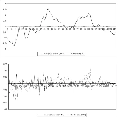
Taylor rule (9) in SW (2003). The systematic part of the optimal policy rate implied by the
modelM137is plotted in …gure 5 (upper part) against the systematic part of the estimated Taylor
rule in SW (2003), i.e. as implied by equation (9) without the corresponding periodical monetary
policy shocks Rt. As becomes clear from the …gure, the implied series on the systematic optimal
rule and the empirical Taylor rule show similar patterns. This similarity is not very surprising
since the empirical Taylor rule considered by SW (2003) mainly includes lagged variables. By
de…nition, the optimal commitment rule, which is derived as an explicit reaction function from the
monetary policy optimization, responds to lagged endogenous variables. Hence, the
backward-looking characteristic that both rules have in common explains to a considerable extent the
similarity in …gure 5.
3 6 These graphs are available upon request.
-0.2 -0.15 -0.1 -0.05 0 0.05 0.1 0.15
1 5 9 13 17 21 25 29 33 37 41 45 49 53 57 61 65 69 73 77 81 85 89 93 97 101 105 109 113 117
measurement errors M1 shocks SW (2003) -2
-1.5 -1 -0.5 0 0.5 1 1.5 2
1 5 9 13 17 21 25 29 33 37 41 45 49 53 57 61 65 69 73 77 81 85 89 93 97 101 105 109 113 117
[image:27.595.94.501.101.507.2]R implied by SW (2003) R implied by M1
Figure 5. Systematic part of instrument rule in SW (2003) vs. optimal rule in M1 (upper part)
and measurement errors M1 vs. monetary policy shocks SW (2003) (lower part)
The lower part of …gure 5 plots the series obtained for the measurement errors, Rt, over the sample
period, i.e. the di¤erence between the actual interest rate movements and the optimal policy rate
implied by model M1. The …gure also shows the monetary policy shocks, R
t, implied by SW
(2003) that includes an empirical Taylor rule. The monetary policy shocks in the benchmark
SW (2003) model generally appear to be of a higher magnitude than the measurement errors in
4
Model Comparison
In this part we compare and rank the models characterized by optimizing monetary policy
behaviour, i.e. the modelsM1andM2, and the benchmark SW (2003) model in which monetary
policy is described by an empirical Taylor rule, based on their marginal likelihood values38
reported in Table 3. In a next step, we compare Bayesian impulse responses for selected shocks
under optimizing monetary policy authorities (M1) to those under SW (2003).
4.1
Marginal Likelihood Comparison
The marginal likelihood of a model can be represented as follows:
p(QT jMi) =
Z
!
p(QT j!; Mi)p(!jMi)d! (22)
where QT contains the observable data series, ! the vector of parameters and Mi the model
under consideration, in our case of three modelsi= 1;2orSW(2003). The likelihood function
p(QT j !; Mi) of the data series is conditional on the parameter vector ! and the modelMi.
p(!jMi)is the prior density of the parameters conditional on the model. Since we use the same
dataset and the same initialization period in the estimation of the three models, the marginal
likelihood values shown in Table 3 are comparable39. As in Schorfheide (2000), we use the
Laplace approximation to approximate the marginal likelihood through the evaluation at the
posterior mode. Table 3 also reports the Modi…ed Harmonic Mean for each model, obtained
through the markov chain monte carlo simulations, which does not di¤er much from the Laplace
approximation. As pointed out by Del Negro and Schorfheide (2006) and Sims (2003), using
the same priors for alternative speci…cations of a model can bias our choice towards one type of
speci…cation. Given this potential pitfall in model comparison within Bayesian frameworks, we
correct for the e¤ect of common priors by estimating and evaluating the models over the training
sample 1970:2-1980:2 as well, and substract accordingly the corresponding marginal likelihood
from the one obtained by estimation over the whole sample period 1970:2-1999:4. The results,
however, turn out to be qualitatively comparable to those reported in the …rst three lines in
Table 3.
Although from the table we can conclude that modelM1 where qw = 0…ts the data better
than modelM2where nominal wage in‡ation is included as a target variable in the loss function,
3 8See Geweke (1998) and Schorfheide (2006) for a detailed discussion on the marginal likelihood function in
Bayesian estimation.
3 9However, it is important to keep in mind that comparison across models based on the marginal likelihood
both models perform relatively worse compared to the benchmark SW (2003) speci…cation of the
model where monetary policy is characterized by an empirical Taylor rule only. This might be
due to the fact that, by introducing optimizing monetary policy into the modelsM1andM2, we
impose a di¤erent and more restrictive structure. This result could also indicate that monetary
policy was not optimal (under commitment) during the sample period. However, it is worth
to point out that in the SW (2003) description of monetary policy behaviour, the Taylor rule
includes …ve parameters, while there are only two monetary policy preference parameters to be
estimated in M1. Hence it is not very surprising that the SW (2003) model with more free
parameters to be estimated performs better thanM1. Therefore, we re-estimate the SW (2003)
model with a slightly di¤erent speci…cation of the empirical Taylor rule (9). We consider the
following rule that responds to only the lagged in‡ation rate and the lagged output gap:
^
Rt= ^
Rt 1+ (1 ) t+r (^t 1 t) +ry( ^
Yt 1
^
Ytp1) (23)
so we drop the second part of reaction function (9) by setting r =r y = 0. The marginal
likelihood of the SW (2003) model under this speci…cation of the Taylor rule worsens to 301:08
(Laplace approximation), with = 0:8894,r = 1:6454andry= 0:1291. Given that it might be
more appropriate to compare the optimal monetary policy model M1 to the SW (2003) model
with a rule like (23), the optimal monetary policy speci…cation is clearly preferred by the data.
4.2
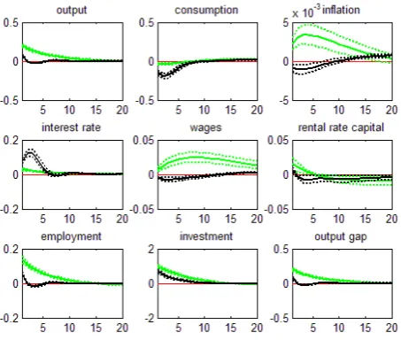
Bayesian Impulse Response Analysis
In this part we visualize the consequences of assuming optimizing monetary policy aurthorities
on the impact and the dynamics of the variables in the case of a supply shock (productivity
shock), a demand shock (equity premium shock) and a cost push shock (price-markup shock)
over a period of 20 quarters. We take the SW (2003) model which includes an estimated
policy reaction function as the benchmark case (green lines) and assess to which extent the
reactions of the variables di¤er when monetary policy minimizes an intertemporal loss function
with one period loss as speci…ed under model M1(dark lines)40. We look at the responses of
nine variables, i.e. output, consumption, in‡ation, interest rate, wages, rental rate of capital,
employment, investment and the output gap. The solid lines are the mean impulse responses,
whereas the dotted lines are the 10% and the 90% posterior intervals.
4 0SinceM1 performs relatively better than M2, we prefer to focus only on the impulse responses obtained
underM1. However, the impulse respones underM2are, with the exception of responses to the equity premium
Figure 6. Productivity shock
Figure 6 shows the responses of the variables to a productivity shock. The interest rate, which
is the policy instrument and responsable for the main di¤erences between the two alternative
model speci…cationsM1 and SW (2003), shows a slightly lower impact and gets more negative
(accommodative) around the third quarter underM1 as opposed to the benchmark SW (2003)
case. Hence consumption and investment both increase to a greater extent, resulting into a
higher increase in output and lower decrease in employment. The output gap does not become
negative, in contrast to the SW (2003) benchmark case, since monetary policy accommodates
the productivity shock more strongly. Although the impact on wages are higher, the rental rate
of capital shows a similar pattern in the two models. Finally, the initial e¤ect on in‡ation is
Figure 7. Equity premium shock
Figure 7 shows the impulse responses of the equity premium shock. The interest rate responds
more strongly to the equity premium shock and gets more positive (more activist policy) around
the third quarter, in contrast to the baseline model, which explains the stronger initial decline in
consumption, the weaker response of investment and hence employment, output and analogically
the output gap. The impact on both wages and rental rate of capital is much weaker and even
turns slightly negative. Therefore, in‡ation responds negatively, however, the e¤ect is very
small.