Calculation of flexoelectric coefficients for a nematic liquid crystal by
atomistic simulation
David L. Cheung, Stewart J. Clark, and Mark R. Wilson
Citation: J. Chem. Phys. 121, 9131 (2004); doi: 10.1063/1.1802231 View online: http://dx.doi.org/10.1063/1.1802231
View Table of Contents: http://jcp.aip.org/resource/1/JCPSA6/v121/i18 Published by the American Institute of Physics.
Additional information on J. Chem. Phys.
Journal Homepage: http://jcp.aip.org/Calculation of flexoelectric coefficients for a nematic liquid crystal
by atomistic simulation
David L. Cheung
Department of Chemistry, University of Durham, South Road, Durham DH1 3LE, United Kingdom and Department of Physics, University of Durham, South Road, Durham DH1 3LE, United Kingdom
Stewart J. Clark
Department of Physics, University of Durham, South Road, Durham DH1 3LE, United Kingdom
Mark R. Wilson
Department of Chemistry, University of Durham, South Road, Durham DH1 3LE, United Kingdom
共Received 21 May 2004; accepted 9 August 2004兲
Equilibrium molecular dynamics calculations have been performed for the liquid crystal molecule
n-4-共trans-4-n-pentylcyclohexyl兲benzonitrile 共PCH5兲 using a fully atomistic model. Simulation data have been obtained for a series of temperatures in the nematic phase. The simulation data have been used to calculate the flexoelectric coefficients esand ebusing the linear response formalism of
Osipov and Nemtsov关M. A. Osipov and V. B. Nemtsov, Sov. Phys. Crstallogr. 31, 125共1986兲兴. The temperature and order parameter dependence of es and eb are examined, as are separate
contributions from different intermolecular interactions. Values of es and eb calculated from
simulation are consistent with those found from experiment. © 2004 American Institute of Physics. 关DOI: 10.1063/1.1802231兴
I. INTRODUCTION
Atomistic computer simulation provides a powerful tool for the investigation of the properties of soft condensed mat-ter systems. Of particular inmat-terest has been the progress made in the simulation of complicated self-ordering systems such as liquid crystal phases.1– 6Here changes in molecular align-mnent can occur on relatively long times scales (⬎1 ns) and accurate force fields are required for simulations to repro-duce the stability of the phases.7–10 In principle the bulk material properties of a system should be available from ac-curate atomistic simulations.11 However, calculation of the physical properties of mesogenic systems in this way is a challenging task. In this paper we use atomistic simulations to study the flexoelectric effect and calculate the flexoelectric coefficients of the nematic liquid crystal n-4-共
trans-4-n-pentylcyclohexyl兲benzonitrile 共PCH5, Fig. 1兲.
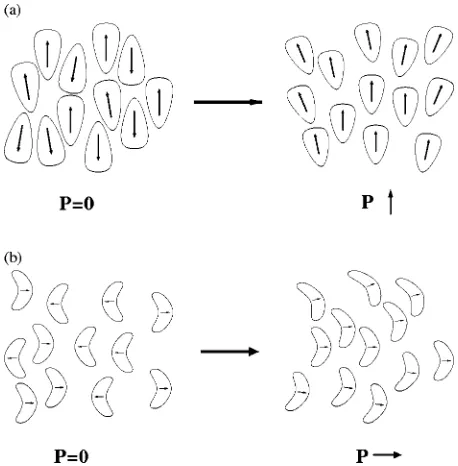
The flexoelectric effect12,13describes the spontaneous po-larization generated by a deformation of the director in a nematic phase composed of molecules, which exhibit shape asymmetry and have permanent dipole moments. A system of wedge-shaped molecules with longitudinal dipoles will exhibit a polarization when the director field is subjected to a splay deformation, as shown in Fig. 2共a兲. Likewise a system of banana-shaped molecules with transverse dipoles will ex-hibit a polarization under bend as shown in Fig. 2共b兲. For rod-shaped polar molecules, such as PCH5, flexoelectric po-larization is expected to result from the effect of splay and bend deformations on transcient dipole dimers of these mol-ecules. Highly polar mesogens such as PCH5 often associate with antiparallel alignment between dipoles.14,15When these dimers are subjected to a splay or bend deformation the di-poles are no longer antiparallel leading to a net polarization, as shown in the top illustration in Fig. 3. The flexoelectric
effect can also be present in quadrupolar mesogens.16 This can arise due to a change in the quadrupole density when the director is splayed, as shown in the bottom illustration in Fig. 3. PCH5 is known also to exhibit strong quadrupolar interactions.17However, the extent to which this mechanism contributes to the flexoelectric effect in systems of rod-shaped molecules such as PCH5 is unknown.
In all cases, a phenomological expression for the flexo-electric polarization per unit volume is given by18
pf⫽e
sn共“"n兲⫹ebn⫻“⫻n, 共1兲
where es and eb are the splay and bend flexoelectric
coeffi-cients. The flexoelectric coefficients appear also in the free energy density of a nematic liquid crystal.19 Here they de-scribe the coupling between director deformations and an applied electric field. This is the converse flexoelectric effect where an applied electric field can distort the director field.12 The flexoelectric effect has a large influence on many phenomena in liquid crystals.20 Technologically it plays a key role in some device applications. Flexoelectric surface switching is important in newly developed bistable displays.21,22 Flexoelectric coupling in chiral and twisted nematic crystals23leads to a linear rotation of the optic axis and also leads to device applications.24 Flexoelectric cou-pling in smectic liquid crystals has been shown to stabilize helical structures.25The flexoelectric effect is present also in lipid membranes.26The direct link between molecular struc-ture and the flexoelectric effect also makes it of fundamental interest.
There have been several experimental studies of the flexoelectric effect 共see Refs. 27 and 28 and references therein兲. However, es and eb are difficult to determine from
experiment. Several theoretical studies have also been
9131
performed29–36 to study the role of molecular structure in determining flexoelectric behavior. These include an Onsager-like theory,29a mean-field theory 共including attrac-tive and repulsive interactions兲,30 and density functional theories.33,34By necessity numerical results from these theo-ries have only been determined for simple models of liquid crystals. Recently more sophisticated theoretical studies have attempted to calculate the flexoelectric coefficients using more realistic models of liquid crystals35or to take the effect of intermolecular interactions into account.36
There have only been three simulation studies of the flexoelectric effect.37– 40Two of these used simple models of wedge-shaped liquid crystal molecules formed by fusing a Gay-Berne molecule and a Lennard-Jones molecule. The first of these studies37,38used a density functional approach based on Ref. 29 while the second used a linear-response formalism.32Qualitatively these studies gave similar results. The bend coefficient was found to be negligible, in line with Meyer’s predictions based on molecular shape.12 However, the values for es differed by an order of magnitude. This
difference is due to the approximations made in calculating the direct correlation function in the density functional
method. Previous studies of the nematic elastic
constants41– 43have shown that approximations made in cal-culating the direct correlation function can lead to large er-rors in the values of the elastic constants. Another study40 compared flexoelectric coefficients calculated from an
atom-istic simulation to theoretical calculations. Again this used density functional theory 共DFT兲 and an approximate direct correlation function, although reasonable agreement between simulation and experimental values of the flexoelectric coef-ficients was reported.
II. THEORY
In this work we turn to the linear-response formalism of Osipov and Nemtsov32 as a means of calculating flexoelec-tric coefficients. es and eb are related to the response func-tion of the system to an orientafunc-tional stress. Specifically the polarization is given by
P␣⫽E␣␥␥␥, 共2兲
where␥␣is the deformation tensor given by
␥␣⫽r␣
, 共3兲
whereis the rotation of the director about the axis given by
[image:3.612.324.549.48.445.2]␣. For small deformations this is
[image:3.612.55.295.52.110.2]FIG. 1. Structure of PCH5 showing dihedral angles␣,,␥, and␦.
FIG. 2. Polarization in a nematic composed of共a兲wedge-shaped molecules with longitudinal dipoles. 共b兲 banana-shaped molecules with transverse dipoles.
FIG. 3. Microscopic mechanism for flexoelectricity in top: symmetric polar liquid crystals; bottom: quadrupolar mesogens.
[image:3.612.60.289.491.724.2]␥␣⫽⑀␣nn 共4兲
withn⫽n/r and⑀␣␥ is the Levi-Citva tensor. The response function E␣␥ is
E␣␥⫽⫺
V
具
P␣⌸␥典
, 共5兲where P is the polarization and
⌸␣⫽⫺
1
2
兺
i⫽jri j␣i j. 共6兲
Here ri jis the intermolecular vector between i and j andi j
is the torque exerted on i by j.
Explicit expressions for the flexoelectric coefficients can be found by writing E␣␥ as
E␣␥⫽E1⑀␣␥⫹E2⑀␣nn␥⫹E3⑀␥nn␣
⫹E4⑀␣␥nn. 共7兲
Multiplying this by the deformation tensor Eq. 共3兲gives
P␣⫽共E3⫺E1兲n␣␥n␥⫺共E1⫹E2兲n␥␥n␣. 共8兲
An expression for es can then be found by multiplying Eq.
共7兲by⑀␥nn␣ and an expression for eb can be found by multiplying Eq. 共7兲by⑀␣nn␥. Doing this gives
es⫽⫺
1
2E␣␥⑀␥nn␣ 共9兲
and
eb⫽⫺12E␣␥⑀␣nn␥. 共10兲
For the purposes of simulation it is convenient to put this in a director based frame of reference. With n⫽zˆ Eqs.共9兲and 共10兲become
es⫽⫺
1
2共Ezxy⫺Ez y x兲, 共11兲
eb⫽⫺
1
2共Ex y z⫺Ey xz兲. 共12兲
III. SIMULATION MODEL AND METHODOLOGY
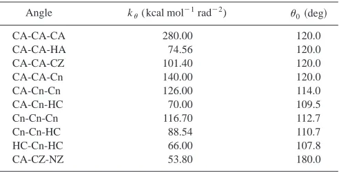
PCH5 molecules共Fig. 1兲were represented using a har-monic all-atom force field of the AMBER form.44The force field parameters were taken from our earlier work7 and are shown in Tables I, II, III, and IV. In Ref. 7 the force field parameters are obtained by fitting to a combination of high-level density functional theory calculations for the intramo-lecular parts of the potential and mointramo-lecular dynamics simu-lations 共to obtain liquid densities and heats of vaporization兲 for the intramolecular parts of the potential.
Molecular dynamics simulations were performed using the DL–POLYprogram version 2.12.45 The equations of mo-tion were integrated using the leapfrog algorithm with a time step of 2 fs. Bond lengths were constrained using the SHAKE algorithm.46 Simulations were performed in the
N pT ensemble using the Nose´-Hoover thermostat and
barostat47– 49with relaxation times of 1 ps and 4 ps, respec-tively. Long range electrostatic interactions were evaluated using an Ewald sum with a convergence parameter of 0.24 Å⫺1 and 11 wave vectors in the x, y , and z directions. The simulations were started from a cubic system of 216 molecules at a gas phase density. The initial state was a highly ordered nematic ( P¯2⬇0.9) with antiferroelectric or-dering. This was then rapidly compressed to a liquid state density 共about 500– 1000 kg m⫺3). An equilibration run of ⬇1 ns was then performed after which statistics were then gathered over 4 ns at each temperature 共300, 310, 320, and 330 K兲. Coordinate data for the calculation of the flexoelec-tric coefficients were saved every 500 time steps 共1 ps兲.
IV. CALCULATION OFes ANDeb
The response function E␣␥ was calculated for each set of saved coordinate data. The polarization p was calculated from
p⫽
兺
iqiri, 共13兲
where qi are the atomic charges and ri are the atomic posi-tion vectors. The sum in Eq. 共13兲runs over all the atoms in the simulation.
The orientational stress tensor is calculated from the torques and center-of-mass positions of the molecules. The torque on molecule i from molecule j, i j, is found from
i j⫽
兺
k [image:4.612.49.298.62.159.2]rc⫻Fk j, 共14兲
TABLE I. Equilibrium bond lengths.
Bond leq共Å兲
CA-CA 1.380
CA-HA 1.080
CA-Cn 1.498
CA-CZ 1.410
Cn-Cn 1.511
Cn-HC 1.088
[image:4.612.315.561.64.189.2]CZ-NZ 1.173
TABLE II. Bond angle bending parameters.
Angle k(kcal mol⫺1rad⫺2) 0共deg兲
CA-CA-CA 280.00 120.0
CA-CA-HA 74.56 120.0
CA-CA-CZ 101.40 120.0
CA-CA-Cn 140.00 120.0
CA-Cn-Cn 126.00 114.0
CA-Cn-HC 70.00 109.5
Cn-Cn-Cn 116.70 112.7
Cn-Cn-HC 88.54 110.7
HC-Cn-HC 66.00 107.8
where rkc is the position vector of atom k in i relative to the center of mass of molecule i, Fk j is the force on k from
molecule j and the sum runs over all atoms in i. Fk jis given
by
Fk j⫽
兺
lFlk, 共15兲
where Flk is the force on atom k from atom l in molecule j
and the sum runs over all the atoms in molecule j . The force between two atoms is the sum of the van der Waals force and the electrostatic force. The van der Waals force is of the Lennard-Jones form
Fklvdw⫽24⑀kl
冋
2kl12
rkl13 ⫺ kl
6
rkl7
册
rˆkl, 共16兲where⑀klandklare the usual van der Waals parameters and
rˆkl is the unit vector along the direction between k and l. As the van der Waals interaction is short ranged this is only evaluated for pairs of atoms less than 12 Å apart, in common with the forces calculated in the simulation.
The electrostatic force was evaluated using Coulomb’s law
Fklelec⫽ 1
4⑀0
qkql rkl
2 rˆkl. 共17兲
Due to the long-range of the electrostatic interaction this is calculated for all pairs of atoms in the system共or their mini-mum image separations兲. For our system containing 9504 atoms there are ⬇45 million atom pairs so this is a large computational task.
V. RESULTS
A. Densities and order parameters
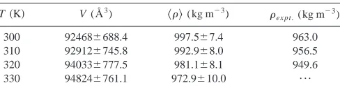
Simulation volumes and calculated densities are shown in Table V. As can be seen there is good agreement between calculated densities and the experimental values50 共better than 5% in each case兲. Shown in Table VI are the values of the order parameter P¯2 calculated from simulation. These were calculated using two different methods. In the first method, the molecular long axis was obtained by diagonal-izing the inertia tensor
I␣⫽
兺
i⫽1n mi共ri
2␦␣⫺
ri␣ri兲. 共18兲
Here ri is the position vector of the ith atom relative to the molecular center of mass and the sum runs over all atoms in the molecule. In the second method, the molecular axis is obtained from the dipole axis. In both cases the director and order parameter are found by diagonalizing the ordering ten-sor
Q␣⫽
兺
i⫽1N
3
2ui␣ui⫺ 1
2␦␣, 共19兲
where uiis the molecular long axis, found from the
[image:5.612.126.486.64.151.2]molecu-lar long axis or the molecumolecu-lar dipole axis. The sum in Eq. 共19兲runs over all molecules in the simulation. Also shown in Table VI are the experimental order parameters found from Raman scattering.51 The simulated order parameters found from the inertia tensor are slightly higher than the experi-mental values at all three temperatures in the nematic phase but are nonetheless in quite good agreement with experi-ment. For the highest temperature studied共330 K兲the simu-lated system remains nematic, which suggests that either some super heating of the nematic phase is occuring in the simulation, or that a combination of system size effects and inaccuracies in the force field mean that we are not able to predict the phase transition 共328 K兲 exactly. Both are likely explanations. Simulations of single site potentials 共where TABLE III. Dihedral angle force constants. All values in kcal mol⫺1.
Dihedral V1 V2 V3 V4 V5 V6
[image:5.612.54.296.630.756.2]CA-CA-CA-CA 0.0 9.51 0.0 0.0 0.0 0.0 CA-CA-Cn-Cn 0.0 0.525 0.0 ⫺0.233 0.0 ⫺0.046 CA-Cn-Cn-Cn 0.0 0.0 0.462 0.0 0.0 0.0 Cn-Cn-Cn-Cn 1.957 0.074 0.028 ⫺0.376 0.039 0.014 Cn-Cn-Cn-HC 0.0 0.0 0.366 0.0 0.0 0.0 HC-Cn-Cn-HC 0.0 0.0 0.318 0.0 0.0 0.0
TABLE IV. Nonbonded interaction parameters.
Atom ⑀(kcal mol⫺1) 共Å兲 q/e
CA 0.070 3.550 ⫺0.122
CA共bridging兲 0.070 3.550 0.0 CA共CA-CZ兲 0.070 3.550 ⫹0.035 CA共CA-Cn兲 0.070 3.550 0.0
CZ 0.150 3.650 ⫹0.395
Cn (CH3) 0.066 3.500 ⫺0.180 Cn (CH2) 0.066 3.500 ⫺0.120 Cn共CH兲 0.066 3.500 ⫺0.060
HA 0.030 2.420 ⫹0.122
[image:5.612.316.560.690.755.2]HC 0.030 2.500 ⫹0.060
TABLE V. Computed densities for simulation PCH5.
T共K兲 V (Å3) 具典(kg m⫺3) ex pt.(kg m⫺3)
300 92468⫾688.4 997.5⫾7.4 963.0 310 92912⫾745.8 992.9⫾8.0 956.5 320 94033⫾777.5 981.1⫾8.1 949.6 330 94824⫾761.1 972.9⫾10.0 ¯
longer simulation runs are possible兲point to some hystersis in cooling/heating through the phase transition, particularly with small system sizes. The most detailed atomistic study of the nematic-isotropic transition conducted top date, for the first three homologs of the phenylalkyl-4-(4
⬘
cyano-benzylidene)-aminocinnamates, was able to predict transi-tions temperatures to within 10⫾5 K.4The order parameters found from the dipole moment are significantly lower than those found from the inertia tensor as well as being lower than the Raman scattering results for temperatures below TNIexpt.. Here the partial charges on the hydrogens in the tail 共which is less aligned than the ring systems兲 have a significant influence on the overall order parameter. We therefore expect the calculated dipolar order parameter to be smaller than the Raman results, where the chromophores共C-N bond and symmeteric phenyl stretch兲are better ordered.
The translational order of the system can be studied through the center of mass radial distribution function 共RDF兲, g(r), and the RDF resolved parallel to the director
g储(r). These are shown in Fig. 4. As can be seen g(r) shows a first solvation peak at⬇6 Å, consistent with a fluid phase and g储(r) remains flat showing no periodic ordering of
mol-ecules. Hence, the simulated liquid crystal phase is nematic and no trace of smectic ordering is seen.
B. Molecular structure
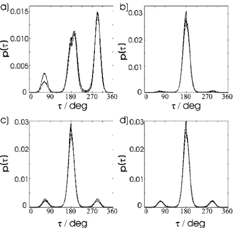
Shown in Fig. 5 are the dihedral distribution functions for some of the dihedrals in the alkyl tail, as shown in Fig. 1. These have an important effect on the overall shape of the molecule. The percentage of dihedrals in the trans and
gauche states can be calculated by integrating over these
[image:6.612.319.558.49.282.2]distributions and these are shown in Table VII. The gauche populations increase with temperature as would be expected. The largest gauche populations occur for the␥dihedral. This
[image:6.612.50.298.75.144.2]FIG. 4. Radial distribution functions for simulated PCH5 at共a兲300 K,共b兲 310 K,共c兲320 K, and共d兲330 K. The solid line shows the radial distribution function and the dashed line shows the radial distribution function resolved parallel to the director.
TABLE VI. Orientational order parameter P¯2 of PCH5 calculated from simulation.
T共K兲 P¯2inertia P¯
2
di pole ¯P
2 ex pt.
[image:6.612.55.297.477.713.2]300 0.68⫾0.02 0.45⫾0.01 0.63 310 0.65⫾0.01 0.47⫾0.00 0.58 320 0.55⫾0.03 0.39⫾0.01 0.50 330 0.51⫾0.04 0.36⫾0.02 0.00
FIG. 5. Dihedral angle distribution functions for the alkyl tail of PCH5. In each graph the solid line indicates the data for 300 K, the long dashed line indicates the data at 310 K, the short dashed line indicates the data at 320 K, and the dotted line shows the data at 330 K.
TABLE VII. Dihedral angle populations for simulated PCH5.共a兲Dihedral angle,共b兲dihedral angle␥, and共c兲dihedral angle␦.
T共K兲
共a兲
trans gauche⫺ gauche⫹
300 97.5% 1.2% 1.3%
310 97.7% 1.2% 1.1%
320 95.5% 2.3% 2.2%
330 95.4% 2.0% 2.6%
共b兲␥
300 85.3% 7.4% 7.3%
310 85.5% 7.2% 7.3%
320 81.8% 8.9% 9.3%
330 79.9% 10.1% 10.0%
共c兲␦
300 86.7% 6.7% 6.6%
310 86.4% 6.9% 6.7%
320 85.3% 7.2% 7.5%
[image:6.612.314.560.546.756.2]is consistent with previous studies2,3and predictions of mean field theory.52 States where the tail is linear, such as the all
trans state and states with␥ in a gauche state and and␦
trans, are of lower energy共and hence of higher probability兲 than states where the tail is nonlinear. The trans populations in the alkyl tail are larger than those for organic liquids such as butane or hexane.7 As butane and hexane are isotropic liquids the dihedral populations are not subject to an ordering mean field.
The molecular shape can also be approximately charac-terized by the equivalent inertia spheroid.2This is a spheroid with an uniform mass density and the same total mass M as the molecule. The dimensions of this give an approximate measure of molecular length, breadth, and width. These are found from the principal moments of inertia Iaa, Ibb, and Icc, i.e., the eigenvalues of the inertia tensor Eq.共18兲. The
lengths of each of the axes 2a, 2b, and 2c are given by
a⫽
冑
2.5共Ibb⫹Icc⫺Iaa兲M ,
b⫽
冑
2.5共Icc⫹Iaa⫺Ibb兲M , 共20兲
c⫽
冑
2.5共Iaa⫹Ibb⫺Icc兲M .
Shown in Table VIII are the principal moments of inertia and the equivalent axes lengths for simulated PCH5. The molecular length 2a shows a slight decrease with tempera-ture, while the molecular breadth and width show a slight increase. This is expected from the dihedral angle distribu-tions and shows that the molecule becomes longer and thin-ner as the system goes further into the nematic phase. This is in accordance with mean-field theory as discussed above. The ratio between c and b is roughly 0.71 across the tem-perature range studied. These results are similar to those ob-tained in a previous atomistic simulation of trans-4-共
trans-4-n-pentylcyclohexyl兲cyclohexylcarbonitrile 共CCH5兲2 where there was a slight change in the axis lengths with tempera-ture within the nematic phase and a larger change on going into the isotropic phase.
C. Polarization
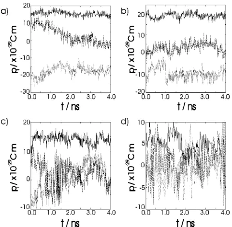
The polarization was calculated from the atomic charges and positions using Eq. 共13兲for each set of coordinate data and the average polarizations are shown in Table IX. The time evolution of the polarization at each temperature is shown in Fig. 6. As can be seen at each temperature there is a small net polarization, particularly directed along the direc-tor. This is a consequence of the finite system size and short simulation lengths 共about 1 ns compared to a time scale of 10–100 ns for molecular reorientation兲rather than any intri-nisic polar ordering.
The reorientational motion of the molecules can be investigated using the reorientational time-correlation functions53,54
Cl共t兲⫽
具
Pl共uˆi共t0兲•uˆi共t0⫹t兲典
, 共21兲 where uˆiis a unit vector defining the orientation of themol-ecule and Pl(x) is the lth Legendre polynomial. Cl(t) for
this is shown in Fig. 7. The decay of C1(t) is slow at all temperatures. This reflects the long times needed for a mol-ecule in the nematic phase to rotate its long axis. This is the reason for the freezing in of a net polarization in this system. All the Cl(t) are similar to those found for other liquid crys-tal systems3 and qualitatively similar to those obtained for simple liquids53,55but with a longer decay time.
To ensure that there is no long-range polar order in the system, the simulation data has been used to calculated the orientational correlation functions g1(r) and g2(r). These are shown in Fig. 8. As can be seen after an initial minima,
g1(r) oscillates about 0. In contrast g2(r) has a maxima at about 5 Å, which is then followed by a decay to a value of about P¯22. The average values of the polarization are shown in Table IX.
D. Flexoelectric coefficients
The flexoelectric coefficients have been calculated using Eqs. 共9兲 and 共10兲and are shown in Table X. Experimental data for es and eb in a nematic is scarce and often
ambiguous28and in many cases there is considerable contro-TABLE VIII. Principal moments of inertia and axes lengths of the equivalent inertia spheroid.
T共K兲 Iaa(⫻10⫺45kg m2)
Iaa(⫻10⫺45kg m2) Iaa(⫻10⫺45kg m2) 2a共Å兲 2b共Å兲 2c共Å兲
[image:7.612.127.487.66.130.2]300 5.197⫾0.034 84.394⫾0.139 86.083⫾0.132 19.74 4.03 2.88 310 5.172⫾0.004 84.312⫾0.022 85.985⫾0.021 19.74 4.02 2.87 320 5.290⫾0.028 83.900⫾0.186 85.896⫾0.166 19.68 4.07 2.89 330 5.315⫾0.024 83.786⫾0.024 85.557⫾0.078 19.67 4.09 2.89
TABLE IX. Computed system polarizations. Here the director lies along the z axis and兩p兩is the magnitude of the polarization vector p.
T共K兲 px(⫻10⫺30C m) py(⫻10⫺30C m) pz(⫻10⫺30C m) 兩p兩(⫻10⫺30C m)
300 3.12⫾4.63 ⫺17.32⫾2.65 15.46⫾1.33 23.92⫾2.58 310 3.24⫾2.51 ⫺10.06⫾2.71 19.54⫾1.38 22.48⫾1.94 320 2.22⫾4.03 1.14⫾4.53 14.07⫾1.62 15.51⫾1.72 330 1.10⫾3.83 ⫺0.52⫾3.55 4.74⫾2.00 7.12⫾2.14
[image:7.612.126.486.692.756.2]versy over the sign of the flexoelectric coefficients. Gener-ally the absolute values for es and eb are of the order of
10 pC m⫺1, which is the same order of magnitude as the results presented here. For PCH5, experimental values for the flexoelectric coefficients have been determined27with es
given as 5.3 pC m⫺1 and eb as 3.3 pC m⫺1 at 303 K, with
quoted errors of about 40%. The temperature dependence of
es and ebwas not fully considered in that study, the
normal-ized difference of the coefficients (es⫺eb)/k2, where k2 is the twist elastic constant, was measured and found to remain constant across the nematic range.
The errors for the individual flexoelectric coefficients in Table X are quite large but several features can be noted from the results. The sign of both es and eb are positive
throughout, with the splay coefficent slightly larger for most temperatures and, within experimental error, the value of the flexoelectric coefficients drop with increasing temperature. This behavior could be rationalized in a number of ways. PCH5 is known to form transcient dipole dimers in both the nematic phase and the pretransitional region of the isotropic phase.15,56 Increases in temperature are likely to reduce the strength of the interactions between the transcient dimers and reduce the dipolar coupling between molecules, thereby re-ducing the flexoelectric effect. It is interesting to note that temperature is likely also to effect the mean molecular dipole moment. As the temperature increases the probability of the tail adopting a gauche conformation increases. The increase in the gauche populations with temperature can be seen from Fig. 5 and Table VII. This could cause the molecule to be-come increasingly bow shaped decreasing the longitudinal dipole moment and increasing the transverse dipole moment. The dipole moment of molecule i, mi, and its longitudinal
[image:8.612.55.295.49.283.2]and transverse components mliand mti are given by FIG. 6. System polarization against time for simulated PCH5 at共a兲300 K,
[image:8.612.318.556.49.284.2]共b兲310 K,共c兲320 K, and共d兲330 K. The solid line denotes the polarization parallel to the director, while the dashed and dotted lines show the polariza-tion perpendicular to the director.
FIG. 7. Orientational time correlation functions Cl(t) (l⫽1,2,3,4) for
simu-lated PCH5 calcusimu-lated using the molecular long axis found from the inertia tensor共3.52兲.共a兲300 K,共b兲310 K,共c兲320 K, and共d兲330 K. In each graph C1(t) is shown by the solid line, C2(t) is shown by the short dashed line,
C3(t) is shown by the long dashed line, and C4(t) is shown by the dotted
line.
[image:8.612.54.293.461.693.2]FIG. 8. Orientational correlation functions g1(r) 共solid line兲 and g2(r) 共dashed line兲at共a兲300 K,共b兲310 K,共c兲320 K, and共d兲330 K.
TABLE X. Calculated flexoelectric coefficients for simulated PCH5.
T共K兲 es(pC m⫺ 1
) eb(pC m⫺1)
300 45.9⫾30.8 51.2⫾11.1
310 80.7⫾15.6 16.5⫾7.5
320 34.8⫾11.0 6.2⫾5.5
[image:8.612.313.561.690.756.2]mi⫽
兺
jqjrj, 共22兲
mli⫽共mi•uˆi兲uˆi, 共23兲
mti⫽mi⫺共mi•uˆi兲uˆi, 共24兲
where qjis the charge on atom j, rj is the position vector of atom j , and uˆiis the molecular long axis found from
diago-nalizing the inertia tensor. The sum in Eq.共22兲runs over all atoms in molecule i. The average molecular dipoles have been calculated and are shown in Table XI. The average longitudinal dipole moment decreases between 300 K and 320 K, and the transverse dipole moment shows a corre-sponding increase. The reduction in mli would again reduce
the strength of the dipolar coupling between pairs of mol-ecules and as a consequence would reduce the flexoelectric coefficients if the mechanism for flexoelectricity involved a disruption of dipolar coupling共top illustration in Fig. 3兲.
The temperature dependence of esand ebcalculated here
can be compared with the temperature dependence predicted theoretically. One such study36 calculated es and eb for the
mesogen 4
⬘
-n-pentyl-4-cyanobiphenyl 共5CB兲, similar in structure to PCH5, with a density functional approach. The molecules were modeled using a dipolar Gay-Berne potential57and the direct correlation function was calculated using a modified Bethe theory58,59 and the Percus-Yevick closure approximation.53 This study found es and eb to beconstant. The model used, however, neglected both molecu-lar flexibility and long-range dipole-dipole interactions, only interactions between nearest and next nearest neighbors were considered. The flexoelectric coefficients of the mesogen 4
⬘
-methoxybenzylidene-4-n-butylaniline 共MBBA兲 have also been calculated using a mean field model.35 es and eb wereboth found to decrease monotonically with temperature using this method.
Comparison with previous simulation results37–39is pos-sible only on the qualitative level due to the vast differences in the models used. PCH5 is far from the idealized pear-shaped molecules used previously. The simulations of Bill-eter and Pelcovits, and Zannoni and co-workers found that the splay flexoelectric coefficient decreases with temperature in agreement to the present results.
The dependence of es and ebon the order parameter P¯2 is shown in Fig. 9. The order parameter dependence of es
and eb from previous studies give ambiguous conclusions.
Early work60 suggested that for dipolar molecules the flexo-electric coefficients are predicted to vary as P¯22, while for quadrupolar molecules the flexoelectric coefficients should vary as P¯2.16Using mean-field theory Osipov30showed that
both P¯2and P¯2 2
dependence should be seen. However, it was also suggested that the effect of molecular flexibility would introduce a P¯2⫺
1
dependence.31 From Fig. 9, a linear depen-dence on P¯22 is seen, indicating that the dipolar flexoelectric effect 共top illustration in Fig. 3兲is likely to be most impor-tant in PCH5.
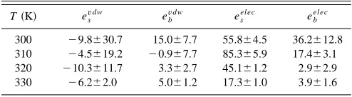
The contributions from the van der Waals and electro-static interactions to the flexoelectric coefficients have also been calculated. These are shown in Table XII. The electro-static contributions to es and eb dominate in each case, as
might be expected. It is interesting to note that the sign of van der Waals’ contribution to esis negative
VI. CONCLUSION
This paper describes the calculation of the flexoelectric coefficients es and eb for a common nematic liquid crystal
PCH5 from atomistic simulation. es and eb have been
calcu-lated at a range of temperatures in the nematic phase. The temperature and order parameter dependence of es and eb
have been examined. Contributions from different intermo-lecular interactions have been determined also.
The calculated values of es and eb are consistent with values determined from experiment. The splay and bend co-efficients are both found to decrease with temperature. This could be explained by a small decrease in the antiparallel dipole correlation in PCH5 as a function of temperature and the small decrease in the longitudinal dipole moment medi-ated by increases in gauche conformations of the alkyl chain. This would be consistent with a dipolar mechanism for flexoelectricity in PCH5, as would the order parameter de-pendence of the results. The electrostatic contributions to es
and eb are found to dominate the van der Waal’s
contribu-tion.
The effect of increasing system size on the calculated values of es and eb has not been investigated in this work.
[image:9.612.322.550.48.165.2]This would be of interest but is beyond our current computer capacity. We note that limited simulations of systems of the TABLE XI. Average dipole moments per molecule calculated using Eqs.
共22兲,共23兲, and共24兲.
T共K兲 具兩m兩典(⫻10⫺30C m) 具兩
ml兩典(⫻10⫺30C m) 具兩mt兩典(⫻10⫺30C m)
300 6.47⫾0.52 3.35⫾1.94 4.97⫾1.58 310 6.46⫾0.53 3.30⫾1.89 5.02⫾1.55 320 6.47⫾0.54 3.13⫾1.83 5.19⫾1.42 330 6.47⫾0.54 3.18⫾1.87 5.14⫾1.47
FIG. 9. Order parameter dependence of esand eb. The triangles show the
[image:9.612.49.301.76.150.2]simulated data and dotted lines show linear regression fits to the data.
TABLE XII. van der Waals and electrostatic contributions to the flexoelec-tric coefficients共in pC m⫺1).
T共K兲 esv dw
ebv dw
es elec
eb elec
300 ⫺9.8⫾30.7 15.0⫾7.7 55.8⫾4.5 36.2⫾12.8 310 ⫺4.5⫾19.2 ⫺0.9⫾7.7 85.3⫾5.9 17.4⫾3.1 320 ⫺10.3⫾11.7 3.3⫾2.7 45.1⫾1.2 2.9⫾2.9 330 ⫺6.2⫾2.0 5.0⫾1.2 17.3⫾1.0 3.9⫾1.6
[image:9.612.314.561.689.757.2]order of 1000 nematogens have recently been performed56,61 and these do provide a better representation of long-range order. However, studies of such system sizes共44 000 atoms for a fully atomistic model of PCH5兲remain extremely com-putationally expensive at the current time. If the large errors can be reduced through the use of larger system sizes, it may well be possible to use simulation to aid in the design of molecules with larger flexoelectric coefficients.
Extension of this work to different mesogens is possible. Calculation of es and eb for a range of different mesogens
would be a good test of the accuracy of the method. It would also be interesting to compare the contributions to esand eb for molecules exhibiting different mechanisms for flexoelec-tricity, e.g., those exhibiting quadrupolar flexoelectricity. The investigation of alternative routes to esand ebwould also be fruitful. Combining the density functional method used in Refs. 37 and 38 with a more accurate method for determin-ing the direct correlation function, such as that recently used by Schmid and co-workers for the calculation of nematic elastic constants62 could provide an alternative route to the flexoelectric coefficients.
1M. R. Wilson, Struct. Bonding共Berlin兲94, 42共1999兲. 2M. R. Wilson and M. P. Allen, Liq. Cryst. 12, 157共1992兲. 3
C. McBride, M. R. Wilson, and J. A. K. Howard, Mol. Phys. 93, 955
共1998兲.
4R. Berardi, L. Muccioli, and C. Zannoni, ChemPhysChem 5, 104共2004兲. 5A. V. Kolmolkin, A. Laaksonen, and A. Maliniak, J. Chem. Phys. 101,
4103共1994兲. 6
S. Y. Yakovenko, A. A. Muravski, F. Eikelschulte, and A. Geiger, Liq. Cryst. 24, 657共1998兲.
7D. L. Cheung, S. J. Clark, and M. R. Wilson, Phys. Rev. E 65, 051709
共2002兲.
8M. A. Glaser, N. A. Clark, E. Garcia, and C. M. Walba, Spectrochim. Acta,
Part A 53, 1325共1997兲.
9E. Garcia, M. A. Glaser, N. A. Clark, and D. M. Walba, J. Mol. Struct.:
THEOCHEM 464, 39共1999兲.
10M. J. Cook and M. R. Wilson, Mol. Cryst. Liq. Cryst. Sci. Technol., Sect.
A 357, 149共2001兲. 11
D. L. Cheung, S. J. Clark, and M. R. Wilson, Chem. Phys. Lett. 356, 140
共2002兲.
12R. B. Meyer, Phys. Rev. Lett. 22, 918共1969兲.
13P. G. de Gennes, Physics of Liquid Crystals共Oxford University Press, New York, 1976兲.
14W. Haase, Z. X. Fan, and H. J. Mu¨ller, J. Chem. Phys. 89, 3317共1988兲. 15M. J. Cook and M. R. Wilson, Liq. Cryst. 27, 1573共2000兲.
16J. Prost and J. P. Marcerou, J. Phys.共Paris兲38, 315共1977兲. 17
M. J. Cook and M. R. Wilson, Liq. Cryst. 27, 1573共2000兲. 18
P. Rudquist and S. T. Lagerwall, Liq. Cryst. 23, 503共1997兲. 19M. P. Allen and A. J. Masters, J. Mater. Chem. 11, 2678共2001兲. 20L. M. Blinov and V. G. Chigrinov, Electrooptic Effects in Liquid Crystals
共Springer, New York, 1993兲. 21
C. Denniston and J. Yeomans, Phys. Rev. Lett. 87, 275505共2001兲. 22A. J. Davidson and N. J. Mottram, Phys. Rev. E 65, 051710共2002兲. 23J. S. Patel and R. B. Meyer, Phys. Rev. Lett. 58, 1538共1987兲.
24A. E. Blatch, M. J. Coles, B. Musgrave, and H. J. Coles, Mol. Cryst. Liq.
Cryst. 401, 161共2003兲.
25M. C˘ epic˘ and B. Z˘eks˘, Phys. Rev. Lett. 87, 085501共2001兲. 26A. G. Petrov, Biochim. Biophys. Acta 85535, 1共2001兲. 27
P. R. M. Murthy, V. A. Raghunathan, and N. V. Madhusudana, Liq. Cryst. 14, 483共1993兲.
28A. G. Petrov, Physical Properties of Liquid Crystals: Nematics, edited by
D. A. Dunmar, A. Fukuda, and G. R. Luckhurst共INSPEC, the Institution of Electrical Engineers, London, 2001兲, p. 251.
29J. P. Stratley, Phys. Rev. A 14, 1835共1976兲. 30
M. A. Osipov, Sov. Phys. JETP 58, 1167共1983兲. 31M. A. Osipov, J. Phys.共France兲Lett. 45, 823共1984兲.
32M. A. Osipov and V. B. Nemtsov, Sov. Phys. Crystallogr. 31, 125共1986兲. 33
Y. Singh and U. P. Singh, Phys. Rev. A 39, 4254共1989兲. 34A. M. Somoza and P. Tarazona, Mol. Phys. 72, 911共1991兲. 35A. Ferrarini, Phys. Rev. E 64, 021710共2001兲.
36
A. V. Zahkarov and R. Y. Dong, Eur. Phys. J. E 6, 3共2001兲.
37J. Stelzer, R. Berardi, and C. Zannoni, Chem. Phys. Lett. 299, 9共1999兲. 38J. Stelzer, R. Berardi, and C. Zannoni, Mol. Cryst. Liq. Cryst. Sci.
Tech-nol., Sect. A 352, 186共2000兲.
39J. L. Billeter and R. A. Pelcovits, Liq. Cryst. 27, 1151共2000兲. 40A. V. Zakharov and A. A. Vakulenko, Crystallogr. Rep. 48, 686共2003兲. 41
J. Stelzer, L. Longa, and H.-R. Trebin, J. Chem. Phys. 103, 3098共1995兲. 42J. Stelzer, L. Longa, and H.-R. Trebin, Mol. Cryst. Liq. Cryst. Sci.
Tech-nol., Sect. A 262, 455共1995兲. 43
M. P. Allen, M. A. Warren, M. R. Wilson, A. Sauron, and W. Smith, J. Chem. Phys. 105, 2850共1996兲.
44W. D. Cornell, P. Cieplak, C. I. Bayly, I. R. Gould, K. M. Merz, D. M.
Ferguson, T. Fox, J. W. Caldwell, and P. A. Kollman, J. Am. Chem. Soc. 117, 5179共1995兲.
45
DL–POLYis a package of molecular simulation routines written by W. Smith and T. R. Forester, copyright The Council for the Central Labora-tory of the Research Councils, Daresbury LaboraLabora-tory at Daresbury, Nr. Warrington, 1996.
46
J. P. Ryckaert, G. Ciccotti, and H. J. C. Berensden, J. Comput. Phys. 23, 327共1977兲.
47S. Nose´, Mol. Phys. 52, 1055共1984兲. 48
W. G. Hoover, Phys. Rev. A 31, 1695共1985兲.
49S. Melchonnia, G. Ciccotti, and B. L. Holian, Mol. Phys. 78, 583共1993兲. 50U. Finkenzeller, T. Geelhaar, G. Weber, and L. Pohl, Liq. Cryst. 5, 313
共1989兲.
51R. Seeliger, H. Haspeklo, and F. Noack, Mol. Phys. 49, 1039共1983兲. 52G. R. Luckhurst, in Nuclear Magnetic Resonance of Liquid Crystals,
ed-ited by J. W. Emsley共Kluwer, Dordecht, 1985兲.
53J. P. Hansen and I. R. McDonald, Theory of Simple Liquids, 2nd ed.
共Academic, New York, 1990兲. 54
D. J. Tildesley and P. A. Madden, Mol. Phys. 48, 129共1983兲.
55M. P. Allen and D. J. Tildesly, Computer Simulation of Liquids共Oxford University Press, Oxford, 1989兲.
56
M. J. Cook and M. R. Wilson, Mol. Cryst. Liq. Cryst. Sci. Technol., Sect. A 363, 181共2001兲.
57J. G. Gay and B. J. Berne, J. Chem. Phys. 74, 3316共1981兲. 58
A. V. Zakharov, Phys. Rev. E 51, 5880共1995兲.
59A. V. Zakharov and S. Romano, Phys. Rev. E 58, 7428共1998兲. 60A. Derzhanski and A. G. Petrov, Phys. Lett. A 34, 483共1971兲.
61Z. Wang, J. A. Lupo, S. Patnaik, and R. Patcher, Comput. Theor. Polym.
Sci. 11, 375共2001兲.
62N. H. Phoung, G. Germano, and F. Schmid, J. Chem. Phys. 115, 7227