GPU-based implementation of real-time system for spiking neural networks

(1)

Theses Thesis/Dissertation Collections

8-1-2009

GPU-based implementation of real-time system for

spiking neural networks

Dmitri Yudanov

Follow this and additional works at:http://scholarworks.rit.edu/theses

This Thesis is brought to you for free and open access by the Thesis/Dissertation Collections at RIT Scholar Works. It has been accepted for inclusion in Theses by an authorized administrator of RIT Scholar Works. For more information, please [email protected].

Recommended Citation

(2)

GPU-Based Implementation of Real-Time System for Spiking

Neural Networks

by

Dmitri Yudanov

A Thesis Submitted in Partial Fulfillment of the Requirements for the Degree of Master of Science in Computer Engineering

Supervised by

Dr. Muhammad Shaaban Department of Computer Engineering

Kate Gleason College of Engineering Rochester Institute of Technology

Rochester, NY August 2009

Approved By:

_____________________________________________ ___________ ___

Dr. Muhammad Shaaban

Primary Advisor – R.I.T. Dept. of Computer Engineering

_ __ ___________________________________ _________ _____

Dr. Roy Melton

Secondary Advisor – R.I.T. Dept. of Computer Engineering

_____________________________________________ ______________

Dr. Leon Reznik

(3)

Thesis Release Permission Form

Rochester Institute of Technology

Kate Gleason College of Engineering

Title: GPU-Based Implementation of Real-Time System for Spiking Neural Networks

I, Dmitri Yudanov, hereby grant permission to the Wallace Memorial Library to

reproduce my thesis in whole or part.

_________________________________

Dmitri Yudanov

_________________________________

(4)

Dedication

(5)

Acknowledgements

(6)

Abstract

Real-time simulations of biological neural networks (BNNs) provide a natural platform for applications in a variety of fields: data classification and pattern recognition, prediction and estimation, signal processing, control and robotics, prosthetics, neurological and neuroscientific modeling. BNNs possess inherently parallel architecture and operate in continuous signal domain. Spiking neural networks (SNNs) are type of BNNs with reduced signal dynamic range: communication between neurons occurs by means of time-stamped events (spikes). SNNs allow reduction of algorithmic complexity and communication data size at a price of little loss in accuracy. Simulation of SNNs using traditional sequential computer architectures results in significant time penalty. This penalty prohibits application of SNNs in real-time systems.

Graphical processing units (GPUs) are cost effective devices specifically designed to exploit parallel shared memory-based floating point operations applied not only to computer graphics, but also to scientific computations. This makes them an attractive solution for SNN simulation compared to that of FPGA, ASIC and cluster message passing computing systems. Successful implementations of GPU-based SNN simulations have been already reported.

(7)

List of Figures

Figure 2.1-1 Morphological structure of a neuron ... 17

Figure 2.1-2 X-ray structure of Gloeobacter violaceus pentameric ligand-gated ion channel [5] 18 Figure 2.1-3 P-type ion pumps transport ions across either cell membranes (a,b) or membranes of intracellular organelles such as the sarcoplasmic reticulum(c,d) [6] ... 19

Figure 2.1-4 Circuit representation of neuron membrane at rest ... 21

Figure 2.1-5 Ion currents during action potential [4] ... 23

Figure 2.1-6 , and during action potential [4] ... 23

Figure 2.1-7 Single ion channel recording [8] ... 24

Figure 2.1-8 Membrane potential waveform with spike rate adaptation [9]. ... 25

Figure 2.1-9 Summary of the neuro-computational properties of biological spiking neurons [10] ... 26

Figure 2.1-10 Gap junction... 27

Figure 2.1-11 Chemical synapse ... 28

Figure 2.1-12 Membrane potential and current traces during process of excitatory synaptic transmission [4] ... 30

Figure 2.1-13 Process of excitatory synaptic transmission: electrical aspect [4] ... 31

Figure 2.1-14 Shunting inhibition and its sculpturing effect on neural signal [4] ... 33

Figure 2.1-15 Spatiotemporal neuronal integration [4] ... 34

Figure 2.1-16 Compartmental division of dendritic tree [11]... 35

Figure 2.1-17 Types of synaptic connections [4] ... 36

Figure 2.1-18 NMDA receptor. Legend: 1. Cell membrane, 2. Channel blocked by Mg2+ at the block site (3), 3. Block site by Mg2+, 4. Hallucinogen compounds binding site, 5. Binding site for Zn2+, 6. Binding site for agonists(glutamate) and/or antagonist ligands(APV), 7. Glycosilation sites, 8. Proton biding sites, 9. Glycine binding sites, 10. Polyamines binding site, 11. Extracellular space, 12. Intracellular space ... 37

Figure 2.1-19 Synaptic current trace at -40 mV and -80 mV. Synapse with blocked NMDA is compared to synapse with functioning NMDA. Shaded area is the difference [4] ... 38

Figure 2.2-1 ∞ and , , , [9] ... 44

Figure 2.2-2 Dynamics of gating variables in HH model [9] ... 45

Figure 2.2-3 Membrane potential and current dynamics in HH mode [9] ... 45

Figure 2.2-4 Circuit of Integrate-and-Fire model [21]. ... 46

Figure 2.2-5 Comparison of biological plausibility and implementation cost of neuron models [10] ... 49

Figure 2.3-1 Simple perceptron ... 52

Figure 2.3-2 Simple ADALINE ... 52

Figure 2.4-1 Spiking Neural Network Model for Edge Detection [30] ... 55

Figure 2.4-2 Image and its firing rate representation with attention area produced by edge detecting SNN [30] ... 56

Figure 2.4-3 Rectangular and Hann windows: time and frequency domains ... 57

(10)

Figure 2.4-5 Spike encoding of signal for one of the subbands [31] ... 60

Figure 2.4-6 Obstacle avoidance and target search in robotics [32] ... 61

Figure 2.4-7 SNN topology for obstacle avoidance and target search in robotics [32] ... 62

Figure 2.4-8 Comparison of number of detected targets [32] ... 63

Figure 3.1-1 Synchronous system: simulation execution flow ... 64

Figure 3.1-2 Delays and cancellations due to quantization error in a synchronous system [1] ... 66

Figure 3.1-3 Asynchronous system: simulation execution flow ... 67

Figure 3.1-4 Dynamics in neuronal systems with STDP: impact of the simulation strategy (clock-driven: cd; event-(clock-driven: ed) on the facilitation and depression of synapses [1] ... 69

Figure 3.1-5 Hybrid system: simulation execution flow ... 70

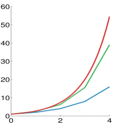
Figure 3.2-1 Illustration of numerical integration for the equation y' = y, y(0) = 1. Blue: the Euler method, green: the midpoint method, red: the exact solution, . The step size is h = 1.0. ... 72

Figure 3.3-1 Diagonal format of sparse matrix representation [39] ... 80

Figure 3.3-2 ELLPACK format of sparse matrix representation [39] ... 81

Figure 3.3-3 Coordinate format of sparse matrix representation [39] ... 81

Figure 3.3-4 CSR format of sparse matrix representation [39] ... 82

Figure 3.3-5 Packetizing of mesh matrices for packet format of sparse matrix representation [39] ... 82

Figure 3.3-6 Packet matrices resulted from packetizing operation [39] ... 83

Figure 4.1-1 Axon hillock circuit [41] ... 85

Figure 4.1-2 Integrate and fire neuron [45] ... 86

Figure 4.2-1 Synaptic transmission using AND gates [47] ... 89

Figure 4.2-2 RT-Spike pipelined architecture [48] ... 90

Figure 4.2-3 SIMD architecture of FPGA-based neuroprocessor with IF neurons [49] ... 91

Figure 4.2-4 Pipeline architecture for Izhikevich neuron [50] ... 91

Figure 4.3-1 Heterogeneous programming [52] ... 93

Figure 4.3-2 Thread hierarchy [52] ... 94

Figure 4.3-3 Hardware architecture of streaming multiprocessor [52] ... 95

Figure 4.3-4 Allocation of blocks to streaming multiprocessors [52] ... 96

Figure 4.3-5 CUDA device memory hierarchy [52] ... 98

Figure 4.3-6 Shared memory access patterns. 1: linear addressing with a stride of one 32-bit word. 2: random permutation. 3: Linear addressing with a stride of three 32-bit words. 4: Linear addressing with a stride of two 32-bit words causes 2-way bank conflicts. 5: Linear addressing with a stride of eight 32-bit words causes 8-way bank conflicts [52] ... 100

Figure 4.3-7 Broadcast access patterns. Left: This access pattern is conflict-free since all threads read from an address within the same 32-bit word. Right: This access pattern causes either no bank conflicts if the word from bank 5 is chosen as the broadcast word during the first step or 2-way bank conflicts, otherwise. ... 101

Figure 4.3-8 Examples of memory access. Left: random float memory access within a 64B segment, resulting in one memory transaction. Center: misaligned float memory access, resulting in one transaction. Right: misaligned float memory access, resulting in two transactions ... 102

Figure 4.3-9 Flowchart of simulation [53] ... 105

(11)

Figure 4.3-1 Izhikevich model current injection results. (Top) Mean simulation time for 1 s simulations with varying error tolerance conditions. (Middle) Adaptive processing statistics. Plots show the mean (over a simulation) number of crossings used by the BS method per step, and the mean and maximum order of the PS method. (Bottom) Simulation accuracy taken as the

reciprocal of absolute voltage divergence between test and reference traces. Line styles as in top panel. PS – Parker-Sochacki method, BS – Bulirsch-Stoer method, RK – Runge-Kutta 4th_order

method. Error tolerance 1E-(condition+1). Time step 0.25ms [2] ... 108

Figure 4.3-2 Block diagram of SNN implementation as a hybrid system ... 110

Figure 5.1-1 Dependency graph for PS step of Izhikevich neuron model. ... 112

Figure 5.1-2 An integration step in update phase of implemented SNN ... 113

Figure 5.1-3 Newton-Raphson iteration ... 115

Figure 5.1-4 Partial warp data parallel operations. ... 117

Figure 5.2-1 Data exchange between update and propagation phases ... 119

Figure 5.2-2 Propagation phase stages ... 121

Figure 5.2-3 Synaptic matrix representation ... 122

Figure 5.2-4 Insertion of new synaptic event into the queue of events of target neuron ... 124

Figure 5.3-1 Interface: block diagram ... 125

Figure 6.1-1 Raster plot of floating point differences between randomly selected membrane potential traces from SNN executed with reference sequential code (run on Opteron 285, 2.6 GHz) and SNN executed on GPU (GTX260). Measurements taken from 100 ms to 200 ms of simulation time for 4 networks of 768 neurons randomly connected (1%, 2%, 3%, and 4% connectivity). Shading: - difference of 1E-2, - difference of zero. Axes: vertical – time steps (0.25 ms), horizontal – neurons. ... 127

Figure 6.1-2 Divergence of membrane potential traces in CPU vs. GPU implementations. 4% randomly connected network of 3840 neurons is used. Comparison is made between the output of sequential program executed on Opteron 285, 2.6 GHz and that from executed on GTX260 device. Measurements are taken from 0 ms to 400 ms of simulation time. Axes: vertical – membrane potential (mV), horizontal – time (ms). ... 128

Figure 6.1-3 Divergence of membrane potential traces in CPU vs. GPU implementations. Closer look at the time segment between 270 and 280 ms from Figure 6.1-2. Axes: vertical – membrane potential (mv), horizontal – time (ms). ... 129

Figure 6.1-4 Spike cancellation in CPU vs. GPU implementation. 4% randomly connected network of 3840 neurons is used. Comparison is made between the output of sequential program executed on Opteron 285, 2.6 GHz and that from executed on GTX260 device. Measurements are taken from 0 ms to 400 ms of simulation time. Axes: vertical – membrane potential (mV), horizontal – time (ms). ... 129

(12)

Figure 6.1-6 Potential trace of source neuron for inhibitory event, which causes spike shift in Figure 6.1-5 (CPU vs. GPU implementation). 4% randomly connected network of 3840 neurons is used. Comparison is made between the output of sequential program executed on Opteron 285, 2.6 GHz and that from executed on GTX260 device. Measurements are taken from 0 ms to 200 ms of simulation time. Axes: vertical – membrane potential (mV), horizontal – time (ms). ... 131

Figure 6.3-1 Scalability of execution time with network size for a range of network densities (0.5% - 8%), 1000 ms of simulated time. Axes: vertical – average execution time (ms), horizontal – network size (number of neurons). ... 136

Figure 6.3-2 Left: size of synaptic queue for each neuron vs. % of connectivity (0.5% - 8%). Right: maximum SNN size possible vs. % of connectivity (0.5% - 8%). ... 137

Figure 6.3-3 Scalability of speedup with network size for a range of network densities (0.5% - 8%), 1000 ms of simulated time. Axes: vertical – average speedup, horizontal – network size (number of neurons). ... 138

Figure 6.3-4 Mean synaptic connections per block with network size, 2% connected network. Axes: vertical – the number of synaptic connections, horizontal – the network size (number of neurons). ... 138

Figure 6.3-5 Scalability of execution time fraction with network size, 2% randomly connected network. Axes: vertical – fraction of execution time, horizontal – network size (number of

neurons). ... 139

(13)

List of Tables

Table 2.1-1Distribution of the major ions across a neuronal membrane at rest: the giant axon of the squid. Nernst potential in reference to extracellular side (chosen as ground by convention) [4] ... 20

Table 6.1-1 Event trace table for the neuron with potential trace presented in Figure 6.1-6 ... 133

Table 6.2-1 Distribution of execution time per computation part for 2% connected network .... 135

(14)

Glossary

ANN Artificial neural network

BNN Biological neural network

CUDA Compute unified device architecture

GPU Graphical processing unit

IZ Izhikevich neuron model

LTD Long term depression

LTP Long term potentiation

PS Parker-Sochacki numerical integration technique

SNN Spiking neural network

(15)

Chapter 1

Introduction

A spiking neural network is a model of a real biological neural network. A building block of an SNN is a mathematical model of a neuron. The choice of this model is design-specific. Neurons communicate with each other by spike events, modeled as time-stamped pulses. A choice of computational system used of SNN modeling defines accuracy of the entire network. There are synchronous systems that tie events to a time grid of simulation flow. Precision of the grid is defined by the magnitude of a time step: the smaller it is the better the precision and accuracy, but more steps per unit of simulation time have to be computed. There are asynchronous systems that update model variables at the time of incoming event and thus, model event time precisely. Two identical SNNs, excited with identical stimuli, but implemented as synchronous and asynchronous systems, do not produce the same spiking pattern unless a time step in synchronous system implementation is extremely small [1], [2].

There are biological mechanisms that require precise timing, for example, spike time dependent plasticity, which is one of the most common research subjects in neuroscience. STDP simulation with system-intrinsic quantization error, introduced by a synchronous system, results in incorrect evolution of network topology due to inability of the system to distinguish between long term potentiation and long term depression [1].

Recently introduced in computational neuroscience Parker-Sochacki numerical integration method [2], applied to biologically plausible phenomenological neuron model developed by Izhikevich [3], provides accuracy that is suitable for precise simulation of SNNs with biological mechanisms that require exact timing. In fact, it was shown that such simulations exhaust full double precision error tolerance requirement [2].

(16)

The text is organized in the following way. Chapter two introduces the reader to neural networks. The first section reviews basic biophysical processes transpiring in biological neurons, such as action potential, synaptic transmission, and neuronal integration. The last part of the section introduces and provides an explanation to the processes requiring precise timing such as spike time dependent plasticity, long term potentiation, long term depression, and classical conditioning. Section two concentrates on modeling aspects of some processes reviewed in the first section, and introduces three most commonly used models of membrane dynamics as well as a simple model of synaptic transmission commonly utilized in SNNs. Section three briefly defines, contrasts, and compares spiking and artificial neural networks. Finally, the last section presents several application examples of SNNs.

The goal of the third chapter is to present modeling approaches to SNNs from the system perspective. The accent is made on time-related aspects of the system modeling: synchronous vs. event driven in the light of two major computational parts of SNNs: update and propagation phases. Suitability of system types for modeling precise time processes, defined in the second chapter, is analyzed. The chapter also provides the insight into important system components such as numerical integration techniques utilized in software and digital hardware models, as well as synaptic data structures responsible for network topology storage.

Chapter four reviews major implementation strategies applicable to SNNs and provides some examples: integrated circuits, programmable logic, and parallel software. Parallel software section is concentrated on GPU implementation, namely CUDA-enabled GPUs. CUDA architecture and its major optimization strategies are reviewed. Examples of works implementing SNNs on GPUs are analyzed.

(17)

Chapter six concentrates on the results and analysis of the system defined in Chapter five from the perspective of execution time, scalability and interfacing with SNN.

(18)

Chapter 2

Introduction to Neural Networks

2.1.

Essential neuroscience

This section reviews basic concepts of neuroscience and introduces definitions that will be used throughout the text. It defines biological basis for neuroscientific modeling.

2.1.1

Membrane Dynamics

[image:18.595.99.501.399.699.2]

A neuron is a building block of nervous system. Morphological structure of a neuron is depicted in Figure 2.1-1.

(19)

From engineering perspective the main functional element of a neuron is its membrane. Made of a lipid bilayer, the membrane has high resistance (1 TOhm for the surface of a typical spinal motor neuron [4]) and therefore, plays a role of the insulator. Placed in aqueous solution it separates extracellular space (outside the cell) from cytoplasmic space (inside the cell) in respect to a nerve cell that it is a part of. The membrane also plays a role of the capacitor (typically 1 / [4]) because the aqueous solution where it resides contains various ion species such as , , ,

, , and organic anions . Concentration of these ion species is different in extracellular and cytoplasmic sides, which results in separation of charges and makes membrane capacitance charged so that the potential across the membrane is between -60 mV and -70 mV relative to extracellular side [4]. This potential is called resting potential with emphasis that no electrical disturbances occur across the membrane. However, the membrane is note opaque because of the presence of electronic devices on its surface called ion channels (Figure 2.1-2).

Figure 2.1-2 X-ray structure of Gloeobacter violaceus pentameric ligand-gated ion channel [5]

(20)

of ion channel), voltage-gated (opening or closing occurs in response to the potential), mechanically-gated (opening or closing occurs in response to pressure or stretch) and resting (these ion channels normally stay open at rest). Ion channels also can be classified in respect to the ions that they permit to pass through the membrane surface (selective permeability).

At rest , and ion channels are open, which decreases membrane resistance approximately by factor of 40,000. Thus, membrane capacitance ( ) leaks charge. However, another kind of electronic devices, ion pumps (Figure 2.1-3), prevent the membrane capacitor from discharging and maintain a steady resting potential because of active ion transport that they generate: is pumped to the extracellular side, is pumped to the intracellular side.

(21)

With each cycle the pump extrudes three ions and brings in two ions, thus producing net outward current (electrogenic property of the pump). Therefore, the pump creates the force that tends to lower membrane potential. However, existence of resting channels results in a passive resistive path for the ions and establishes resting potential as an equilibrium point.

As a consequence, there are two forces that impact ion dynamics of the membrane:

1) Chemical driving force on each individual ion that depends on concentration gradient of that ion species across the membrane. This force is controlled by density of resting ion channels on the membrane surface and ion pump activity. The potential between ions of the same type that is established due to concentration gradient force, assuming that all other ion species are absent, is called equilibrium or Nernst potential.

2) Electrical driving force defined by the potential differences across the membrane as a result of membrane capacitor charge. This force depends on the total charge separated by membrane, which depends on concentration gradient of each ion type on both sides of the membrane and membrane surface area. Consequently, both forces are interdependent.

At its steady state forces and concentration gradients are balanced, net ion flux across the membrane is zero, and its resting potential is about -60 mV (Table 2.1-1).

Ion species Concentration in

cytoplasm,

Concentration in extracellular fluid,

Nernst Potential,

ln

(mM) (mM) (mV)

400 20 -75

50 440 +55

52 560 -60

Table 2.1-1Distribution of the major ions across a neuronal membrane at rest: the giant axon of the squid. Nernst potential in reference to extracellular side (chosen as ground by convention) [4]

(22)

The system at its steady state can be expressed as an electrical circuit (Figure 2.1-4).

Figure 2.1-4 Circuit representation of neuron membrane at rest

In this circuit it is assumed that equilibrium potential of ion species doesn’t change if resistive load is applied to the species source, and therefore, the source can be modeled as a voltage source or a battery with voltage across it. Polarity of this

battery is defined by concentration gradient force relative to the extracellular side and ion species carrier charge. Resting channels are modeled as conductances that provide paths for steady state currents . Currents due to ion pump are shown as

, _{, and polarized membrane capacitance is} _. _{is not shown because its value is}

zero since its Nernst potential is equal to the resting potential, and therefore, there is no net force that drives ions in or out of the cell. An additional conductance path for other possible ions that model leakage current is omitted for simplicity. As a result, resting potential can be represented by the following equation [4]:

(2.1-1)

(23)

way that there are more ions on the extracellular side. ions are pumped to the cytoplasmic side and leak away from the cell through again due to chemical driving force. Their concentration is balanced so that there are more ions in cytoplasmic side. As a rule, at rest < . Thus, electrical and chemical forces affecting ions are larger than those of ions. Besides, electrogenic pump property generates more current than current. This current balances with equivalent current through

resting channels. As a result, the overall balance point (resting potential) is shifted towards the negative side since current is directed inward.

Artificially injected into a cell current disturbs the balance and moves the

potential in either direction: up if is inward, and down if is outward. Because net

current ( , ) follows , resting potential is said to be reversal potential, since the current changes its direction about its value. Reversal potential can be viewed as a voltage source in Thevenin equivalent circuit, which can be obtained from the circuit in Figure 2.1-4.

If membrane is disturbed electrically due to artificially injected current, so that net current is inward and increases (depolarization), the system changes its behavior. Depolarization may result in membrane potential reaching threshold potential of voltage-gated channels. In order to reach this threshold the membrane capacitance has to accumulate some charge, which results in instant capacitive current (Figure 2.1-5, ). If this threshold is reached, ion channels start opening rapidly providing influx of ions into the cell.

During depolarization voltage-gated channels open stochastically. However, when combined they produce aggregated exponential current influx (Figure 2.1-5, ). Their stochastic behavior is defined by their density on the surface of the membrane. The density is the highest at the part of a cell called axon hillock (Figure 2.1-1).

(24)

consequence, net current into the cell changes its direction from inward to outward (Figure 2.1-5, right trace) and the membrane potential returns to its resting potential value (repolarization). As a rule, the membrane potential falls slightly below its resting potential value (hyperpolarization) because of prolonged opening of channels.

Figure 2.1-5 Ion currents during action potential [4]

(25)

Hyperpolarization is necessary in this case for faster deinactivation (returning to active state) of channels since they inactivate (become inactive) during depolarization. Once channels are deinactivated they can activate again if membrane potential exceeds the threshold.

Because channels stay inactive for some time, it is not possible to excite a neuron. This period of time is defined as absolute refractory period. There is also a relative refractory period, followed by absolute refractory period, during which it is possible to excite the cell with stronger stimuli.

The overall result of this process, namely, rapid depolarizing current (Figure 2.1-5, ) followed by delayed rectified repolarizing current (Figure 2.1-5, ) combined with inactivation of voltage-gated channels, is a positive spike of membrane potential known as action potential (AP) [7].

Each individual ion channel opens in all-or-none fashion for variable duration of time that is unpredictable and determined by local random thermal and chemical activities on the nanoscale level. Thus, its behavior is stochastic (Figure 2.1-7).

Figure 2.1-7 Single ion channel recording [8]

(26)

The variety of ion channels is not limited to voltage-gated and ion channels. There are thousands of various ion channels that shape action potential. Having such a variety of ion channels nervous system achieves rich information processing capabilities with computation done by spike generation and synaptic transmission (discussed further) and communication done by spikes.

An example of another type of voltage-gated channels is M-type (muscarine-sensitive) channels, which contribute to the effect of spike frequency adaptation, SFA (an ability of a neuron to accommodate or adapt to increased stimuli and either stop or reduce firing) depicted in Figure 2.1-8

Figure 2.1-8 Membrane potential waveform with spike rate adaptation [9].

M-type channels require several hundred milliseconds to activate in response to depolarization. As a result, they provide an additional conductance path for ions, which leads to reduction of membrane input resistance, charge leak, and increase in time spent for accumulation enough charge on the membrane capacitor in order to reach the threshold and trigger the action potential.

(27)

Figure 2.1-9 Summary of the neuro-computational properties of biological spiking neurons [10]

2.1.2

Synaptic transmission

(28)

lower than that of chemical synapse. The primary function of electrical synapses is to provide firing synchrony between connected cells, especially between large groups of neurons performing the same task.

Figure 2.1-10 Gap junction

(29)

Figure 2.1-11 Chemical synapse

Receptor and its effector, an ion channel, can either compose the same unit, in which case this unit is a ligand-gated ion channel also known as ionotropic receptor, or they can be distinct units. In the latter case, the effector can be located anywhere on the membrane. It is activated via second messenger proteins synthesized and freely distributed across the cell because of receptor activation, and receptor is said to be metabotropic. After neurotransmitter is released, it diffuses out of the cleft and rapidly hydrolyses. Channels start to close in a random fashion (Figure 2.1-11, 6), which results in exponential decay of local membrane conductance.

(30)

Spread of neurotransmitter after its release determines the impact and delay of signal transmission: it can be directed and fast as in case with synaptic cleft and active zone, or it can be more diffuse and slower playing a role of modulator.

Because each vesicle contains thousands of neurotransmitter molecules and there are only a few required for a single receptor to activate, relatively weak pre-synaptic spike can invoke a normal increase in post-synaptic conductance. Thus, the system provides a way for discrete signal propagation without signal loss.

The relation between receptor type and transmitter type is ONTO: several distinct receptor types (even with distinct functions) can utilize a single transmitter type. Receptor function can be either excitatory or inhibitory and its activation function depends on whether it is ionotropic (mostly responsible for reflexes) or metabotropic (mostly responsible for learning).

In addition to the ligand-gated channels, synaptic cleft may contain voltage-gated channels ( channels, for example) that enhance localized increase in membrane conductance, and contribute to local subthreshold potential spike and excitability of the cell.

The main differences between action potential and localized potential spike at the synaptic cleft are the following:

(31)

Ionotropic receptors open in response to neurotransmitter binding from extracellular side. The effect of this opening is limited since it is not regenerative and doesn’t have all-or-none action. Channels open rapidly elevating membrane conductance and potential locally due to the abrupt increase in neurotransmitter concentration, but they close with exponential decay according to their stochastic properties (Figure 2.1-12, upper trace). At the same time, single-channel conductance stays constant and behaves as a switch.

Figure 2.1-12 Membrane potential and current traces during process of excitatory synaptic transmission [4]

(32)

in the cleft is indicative of concentration gradient force on this ion and is the same across the membrane. However, since receptors may be permeable to several ion species each at specific conductance value (for example in neuromuscular junction receptors conduct both and ions), the reversal potential for all ion species in the cleft is most likely to be different from that of resting potential (reversal potential for the membrane at rest). Thus, similar to equation (2.1-1) the reversal potential of receptors in the cleft can be found as a weighted average of equilibrium potentials of ions that these receptors are permeable to, where the weights are specific ion conductances, intrinsic properties of the receptor type. In the case of neuromuscular junction the reversal potential is zero.

Figure 2.1-13 Process of excitatory synaptic transmission: electrical aspect [4]

The process of excitatory synaptic transmission from the perspective of post-synaptic cell can be described using equivalent electrical circuit (Figure 2.1-13) and corresponding waveform (Figure 2.1-12) as a sequence of several steps: 1) At steady state post-synaptic potential is equal to resting potential. Synaptic equivalent conductance

(33)

peak. 4) changes its direction returning the acquired charge to extracellular side through resting channels. slowly decays to its resting value.

Due to the fact that leakage current takes over only in step (3) ratio of value at its peak to (the equivalent resting conductance) value defines the magnitude of potential peak: the larger this gap the more charge is deposited during step (2), and the larger EPSP peak.

Among most common excitatory ionotropic receptors are L-glutamate activated receptors: NMDA receptor (N-methyl-D-aspartate) permeable to , , ; and non-NMDA receptors (permeable to and ): AMPA receptor ( -amino-3-hydroxy-5methyliosoxazole-4-propionic acid) and kainite receptor.

Among most common inhibitory receptors are GABA activated ionotropic

GABA channels and metabotropic GABA receptors that activate channels.

The sequence of steps describing excitatory synaptic transmission is applicable to inhibitory synaptic transmission. However, in this case ion channel species are (for

GABA ), and is an outward current. Indeed, according to Table 2.1-1, chemical

concentration gradient force affects ions and drives them inside the cell resulting in negative charge influx as a response to increased , which corresponds to the outward positive current. However, reversal potential of the channels corresponds to equilibrium potential of ions since channels permit only this type of ions. This potential is the same (or slightly less) as membrane potential at rest, which results in zero or small current through the channels. How does opening of channels in inhibitory synapse with no current can affect membrane potential? The explanation of this process is described in the next section.

2.1.3

Signal integration and modulation

(34)

The primary function of neuronal integration is summing ion currents from synapses of opposite polarity. As it was shown in section 2.1.2, of ionotropic GABAergic synapses is near resting membrane potential, and increase produces none or small outward . However, in the presence of simultaneous , the effect of increased is prominent, because in this case increased overall membrane conductance prevents some part of from depositing on membrane capacitance as a charge and instead leaks away from the cell as , although using different ion species. Thus, inhibitory synapse provides a conductive shunting path for any excitatory current in the cell. This process is called shunting inhibition (Figure 2.1-14). Shunting inhibition patterns temporal activity of spiking neurons (sculpturing).

Figure 2.1-14 Shunting inhibition and its sculpturing effect on neural signal [4]

Because reversal potential of receptor is very close to resting potential, it is relatively easy for ions to accumulate inside of a cell with successive inhibitory events. This, however, may reverse the action of synapse from inhibitory to excitatory if accumulation achieves the point when concentration gradient of reverses the direction of chemical force.

(35)

Figure 2.1-15 Spatiotemporal neuronal integration [4]

Larger membrane capacitance holds more charge and requires more time for charging and discharging, which results in longer time constant. Capacitive current is usually the fastest (Figure 2.1-12), and leakage conductance is smaller than synaptic

conductance. Therefore, it is primarily that determines the time of depolarization in

case of EPSP, and determines time of repolarization. As a consequence, the

membrane with larger repolarizes slower and is more likely to generate action potential as a result of consecutive EPSPs.

(36)

approximately constant lateral (series) resistance and associated transverse (shunt) membrane RC sub-circuit (Figure 2.1-16).

Figure 2.1-16 Compartmental division of dendritic tree [11]

Thus, a passive component of dendritic tree can be viewed as a network of non-inductive leaky transmission lines. If length constant of this line is such that its shunting properties are weak relative to conductive properties of lateral component (smaller transverse capacitance and conductance, but larger lateral conductance), then current loss from the source (synapse) to axon hillock is minimal, and length constant is said to be large. With larger length constant more current is delivered to axon hillock, more chances are that membrane produces a spike. The effect is opposite with smaller length constant.

(37)

Figure 2.1-17 Types of synaptic connections [4]

Axosomatic synapses are usually inhibitory: they provide shunting path for currents flowing from dendritic tree to axon hillock. Axondendritic synapses provide excitatory integrative function. Axo-axonic synapses are usually modulatory: they control neurotransmitter release. The role of modulatory function in synaptic integration is explained further.

Signal modulation is achieved by a variety of means. Simple signal modulation resulting from activation of voltage-gated M-type channels and consequent effect of SFA has been shown in section 2.1.1.

(38)

Figure 2.1-18 NMDA receptor. Legend: 1. Cell membrane, 2. Channel blocked by Mg2+ at the block site (3), 3. Block site by Mg2+, 4. Hallucinogen compounds binding site, 5. Binding site for Zn2+, 6. Binding site for agonists(glutamate) and/or antagonist ligands(APV), 7. Glycosilation sites, 8. Proton

biding sites, 9. Glycine binding sites, 10. Polyamines binding site, 11. Extracellular space, 12. Intracellular space

(39)

Figure 2.1-19 Synaptic current trace at -40 mV and -80 mV. Synapse with blocked NMDA is compared to synapse with functioning NMDA. Shaded area is the difference [4]

(40)

morphological changes, such as enlargement of related dendrite, creation of new spines, and others [13]. Overall this process of the increase in synaptic strength is called long term potentiation (LTP), which is a form of synaptic plasticity (an ability of synapses to change its strength in response to spikes). The reverse process, weakening of synaptic strength, is called long term depression (LTD).

Notwithstanding the fact that LTP and LTD have opposite effects on a synapse, they are closely related, since both of these processes originate from NMDA receptor properties. General rule for excitation is the following: if pre-synaptic EPSP arrives a few milliseconds before post-synaptic cell generates AP, then synapse exhibits LTP; however, if pre-synaptic EPSP arrives few milliseconds after post-synaptic cell generates AP, then the synapse exhibits LTD. This type of synaptic plasticity is called spike time dependent plasticity (STDP). It is one of the most controversial and actively researched types of plasticity. The controversy comes from various aspects: for some neurons the rule is inverted; there is a large variability in timing window between LTD and LTP among neurons and synapses of the same neuron, and others [12]. Besides, STDP is affected by various processes: spiking frequency, threshold of depolarization, distance of synapse from axon hillock, reinforcement of back-propagating AP strength, AP width [14], and others.

At the same time, the general accepted cause of LTD and LTP induction in STDP is difference in current transients: brief and strong postsynaptic elevations signal LTP; smaller, more prolonged transients induce LTD. Simplified explanation of this can be done on the basis of dynamics. Voltage-dependant channels (VDCCs) located on a membrane on the branches of a dendritic tree generate background

(41)

It is imperative to understand that above explanation is rather hypothetic, because STDP is the area of active ongoing research, and new, unknown before, contradicting results actively contribute to the overall picture of STDP as a much more complex process.

On a long term due to the response properties of NMDA receptors LTP is spike frequency-dependent: high frequency stimulation leads to LTP, whereas low frequency stimulation leads to LTD. Brief high-frequency stimulation results in strong postsynaptic depolarization and NMDA receptor activation, whereas sustained low-frequency stimulation evokes less NMDA receptor-dependent influx leaving the rest for VDCCs.

Another interesting property of NMDA receptor is dynamic reduction of glutamate affinity as a response to glutamate exposure in the presence of blocker in NMDA channel. As a consequence, it establishes the size of a time window for efficient LTP: depolarization immediately after glutamate release opens channel more efficiently than later in time [15].

NMDA is not the only mediator of LTP and LTD, neither its dynamics is precisely described in this text, since process of STDP is not completely understood.

One of the most important contributions of STDP is classical conditioning. Classical conditioning is based on associative learning. It involves two types of stimuli/response [16]: 1) Unconditioned stimuli invoke innate, often reflexive response, such as salivation when sensing food. 2) Conditioned stimuli are neutral, for example, hearing a ringing bell. After both food and ringing bell are presented, for example, to a dog several times, eventually the dog learns to salivate in the presence of ringing bell without presence of food.

(42)

Compared to ionotropic receptors, in which receptor and effector constitute the same unit, metabotropic receptors activate/deactivate their effectors via chain of biochemical processes transpired in cytoplasm. The processes employ second messengers. As a result, activation takes longer and its duration lasts longer as well. Besides, the range of activation is global to the cytoplasm due to freely distributed second messengers.

Another property of metabotropic receptors is the duality of their action: under different conditions they can decrease or increase channel opening. The main function of metabotropic receptors, however, is modulatory synaptic actions, such as changes in resting potential, input resistance of the cell, time constants, threshold potential, action potential duration, firing patterns, and others. These actions can be typified by effector channel targets and the corresponding effects they produce: 1) Channels at pre-synaptic axon terminals (transmitter release); 2) Ionotropic receptors (synaptic potential); 3) Resting and voltage-gated channels (excitability and firing).

An example of type (3) modulation is disabling or decreasing effect of spike frequency adaptation by means of metabotropic muscarinic acetylcholine- (ACh) activated receptors. These receptors are present along with ionotropic nicotinic receptors in excitatory synapses. Upon synaptic transmission they signal via second messengers to M-type channels and as a consequence, disable their activation. The result of this is increase in input membrane resistance, increase in current required for cell depolarization, increase in cell excitability, and reduction of spike rate adaptation effect.

(43)

2.2.

Neuron models

In order to reverse-engineer biophysical processes described in section 2.1 using different implementation technology for the purpose of their application in various fields, it is essential to understand which processes nature tries to mitigate and how and which ones are essential mechanisms that contribute to the variety of system dynamics. In this sense it might be possible to avoid effects mitigated by the nature if implementation technology allows that. However, caution has to be taken, because not all processes are fully understood and the ones that seem unwanted now may become having considerable contribution in the future.

The world of neuronal models is much more diverse compared to what is presented in this text; however it is very far from being diverse if compared to the variety of biochemical processes, small part of which is presented in section 2.1. There are models that consider each individual ion channels [18], [19] and model membrane surface dynamics as accurate as possible. There are stochastic spiking neuron models [20]. There are compartmental models that consider impact of dendritic tree on internal current dynamics of the soma by slicing a cell into compartments [11]. There are single-compartment models that assume all synapses terminate on soma and impact axon hillock directly. It is the application targeted by the model and its requirements that determine the model choice.

(44)

2.2.1

Hodgkin-Huxley model

HH model [7] is considered the most biologically plausible and intuitive (its variable set has biological interpretation). Developed by pioneers, who discovered mechanics behind action potential, the model is still widely used today if accuracy of neuron simulation is of the first priority. The equations of the model are the following:

,

, ,

,

(2.2-1)

In this equation set is membrane capacitance, is membrane potential. A set of currents , , , is composed of injected current, and currents,

(45)

, , are obtained by experimental fitting during matching to the desired curve. Typical result of fitting produces and such as in Figure 2.2-1.

Figure 2.2-1 ∞ and , , , [9]

In Figure 2.2-1 time constant of gating variable has evident bump about

70 . As it is seen from the equation, variable due to its negative feedback models inactivation process (halting flow, discussed in 2.1.1). This corresponds to engaging inactivating gate in voltage-gated channels. However, in order to repel this gate from the channel (deinactivate) faster, it is necessary to hyperpolarize the cell. Thus, this bump corresponds to faster recovery of within this potential vicinity – the process of deinactivation.

The model variables can be used either as current densities or as absolute values. In the former case, variables , , are expressed as a value per unit area of the

membrane. Resting potential is not explicitly defined, but it is assumed that is at the steady state.

(46)

depolarizing current , the resulted increase in membrane potential increases and decreases . At some implicit threshold potential value both and

are above zero and such that gating variables and lagging behind these values with rates and slowly open . This, in turn, results in larger increase of , pushing to 1 and to 0. However, the rate with which these variables change are different, namely, is more than (Figure 2.2-1) and therefore, approaches slower than does (Figure 2.2-2).

Figure 2.2-2 Dynamics of gating variables in HH model [9]

Thus, the effect of negative feedback from lags behind the effect of positive feedback from resulting in abrupt influx of (Figure 2.2-3).

Figure 2.2-3 Membrane potential and current dynamics in HH mode [9]

(47)

2.2.2

Integrate-and-fire models

This set of models is based on modeling of subthreshold membrane potential dynamics excluding explicit mathematical description of membrane voltage-gated and conductances [21]. As a result, in its simplistic form, called leaky or passive integrate-and-fire, the model can be described as a parallel resistive-capacitive network (Figure 2.2-4, soma part).

Figure 2.2-4 Circuit of Integrate-and-Fire model [22].

Mathematically, a simple passive IF model is described by the following set of equations:

, ,

:

(2.2-2)

In these equations: and are injected and leakage currents of the cell

(48)

resting potential of the cell, and are firing threshold potential and firing time respectfully, is a reset potential after firing, .

With added spike frequency adaptation discussed in 2.1.1 model equations become:

, ,

,

: 1 ∆ ,

2 after

(2.2-3)

In these equations newly added variables are: is adaptation current that

models dynamics and spike rate adaptation, is conductance, is time constant that defines dynamics over time.

The model operates in the following way: certain part of the current is integrated on a membrane capacitor as a charge forcing membrane potential to rise. Another part of this current simply leaks through linear resistor 1/ as . Sometime after the membrane potential elevates beyond the threshold potential

(this time is defined by the firing time ) is reset to and the

process repeats. However, there is another part of the membrane current, , which is

subtracted from and leaks through non-linear conductance . The value of is defined by the firing rate since is incremented by some value ∆ after each spike. At the same time, decays exponentially during the time between the spikes. As a consequence, mean value of ∆ and therefore, mean value of is well defined after

several spikes assuming that is at the steady state. If changes then adapts to its new mean value after several spikes (Figure 2.1-8).

(49)

One of the major benefits of this model is its simplicity and small execution time if used in neural networks based on numerical integration methods. However, biological plausibility of this model in respect to the gamut of spiking patterns is limited.

2.2.3

Izhikevich model

IZ model is relatively new [3], however, it’s been acquiring active use in neuroscientific computational systems. It is derived according to bifurcation theory and normal form reduction [23]. The goal of this model is to achieve biological plausibility comparable to that of HH model, but at the same time be lightweight computationally. The author claims that the model provides biological functions comparable to those of HH model. However, the model variable set doesn’t have biological interpretation. Thus, the model is said to be phenomenological. The model equations are the following [24]:

,

_:

(2.2-4)

In these equations: is membrane capacitance, is membrane potential, is resting membrane potential, is threshold potential, is action potential

escape limiting value, is recovery variable that models and currents, is injected current, is a parameter that describes the time scale of recovery variable , is a parameter that describes sensitivity of to the subthreshold fluctuations of membrane potential, is a parameter that describes after-spike reset value due to hyperpolarizing outward current and is typically set to a value less than , is a parameter that describes after-spike reset of , describes sensitivity of to the fluctuations of itself.

(50)

accelerates membrane potential dynamics, which results in a spike. At the same time, this high spiking value of accelerates , which provides negative feedback to and to itself playing a role of ionic current at that time. Compared to , which provides quadratic dependence to its acceleration, the equation that governs has only 1st power dependence on . Thus, shaped by and , follows . As a consequence, has to be artificially reset in order to keep it in the plausible range. Thus, once reaches , it is reset to

value . At the same time, is incremented rather than reset, and thus, it “memorizes” previous spike dynamics and affects the refractory period. Variable without term

would play a similar role as plays in IF mode. However, this term gives it the functionality of controllable response to membrane potential dynamics, and therefore, enriches the model with types of dynamics such as intrinsically bursting, chattering, fast spiking, low-threshold spiking, thalamo-cortical spiking, resonating and other dynamics [3].

A chart describing biological plausibility and computational complexity of models assembled by the author of IZ model is presented in Figure 2.1-1.

Figure 2.2-5 Comparison of biological plausibility and implementation cost of neuron models [10]

2.2.4

Simple post-synaptic conductance model

(51)

type of conductance does not provide complex NMDA response, neither it counts for the synaptic delay (synaptic delay can be merged with axonal transmission delay) nor for finite slope of conductance rise (see section 2.1.2), it provides a simple way to interact with a membrane equation of any membrane model described above. This interaction is done by adding another current term to the capacitor equation of corresponding

membrane model [25]:

(2.2-5)

where - membrane potential, - synaptic current, - excitatory conductance, – inhibitory conductance, - excitatory synaptic receptor reversal

potential, – inhibitory synaptic reversal potential, and – excitatory and

inhibitory decay rate constants respectively.

If pre-synaptic spike arrives, either conductance or increments by its maximum conductance value (aka weight), depending on a type of synapse. Consequently, magnitude of increases and participates in membrane dynamics (model of which can be HH, IZ, IF, or any other). At the same time, conductance starts to decay exponentially with rates or .

(52)

2.3.

Neural network types

This section provides brief comparison of spiking neural networks and artificial neural networks.

2.3.1

Spiking neural networks

Spiking neural networks (SNNs) are type of BNNs with reduced dynamic range of transmitted signal, namely, signal at the axon terminal. Because this signal is composed of spikes, its magnitude can be approximated by zero or one in the time domain: zero when there are no spikes and one when there is a spike. Thus, the signal consists of the pulse train with variable inter-spike intervals.

Such a dramatic reduction in signal dynamic range is possible due to the properties of a synapse, signal transfer function of which can be approximated to an increase in membrane conductance followed by its exponential decay in the post-synaptic neuron as a response to arrived action potential in the pre-synaptic neuron. However, the important information about the time of arriving spike is preserved in SNNs. Membrane dynamics is also preserved in the form of membrane potential model.

Because SNNs inherit time domain from BNNs, they inherit the opportunity to model time-dependent phenomena of BNNs. Examples of phenomena are: temporal binding due to synchronized firing [26], STDP and other dependent types of plasticity, LTD, LTP, classical conditioning. Besides, axonal delay is an important temporal variable that participates in learning [27].

(53)

2.3.2

Artificial neural networks

Typical example of neurons involved in artificial neural networks (ANNs) are perceptron (Figure 2.3-1) and ADALINE (Figure 2.3-2).

Figure 2.3-1 Simple perceptron

(54)

Perceptron computes weighted sum of its inputs ∑ and produces an output based on the result of its activation function . There is a variety of activation functions: step, sign, sigmoid, linear. As a rule, the result is between -1 and 1. Perceptron-based ANNs are used as classifiers. Training is required for obtaining weights. Training of multi-layered perceptron-based ANNs is usually accomplished with backpropagation algorithm, in which an error taken as difference between the output and desired output is propagated back in the network and used for weights ajustment [28].

ADALINE (adaptive linear neuron) is similar to perceptron with threshold or liner function. However training of ADALINE is accomplished based on the output taken before the activation function.

After training ANNs are used in various applications: classification, estimation, filtering, and others.

Compared to SNNs, artificial neural networks (ANNs) operate on signal without relation to its time. Considering the fact that a neural signal consists of spikes, it is valid to assume that ANNs abstract signals to their steady state mean firing rate, consequently reducing the parametric space of the neuron model. This simplification, however, makes ANNs static and prohibits their application where time factor matters.

Practically all dynamic processes sensed by biological organisms and the reaction to these processes are out of ANNs application range. A few examples of such processes are sensory system of electric fish, auditory system of bats, visual system of flies, rat's position in a maze and many others [29]. Besides, ANNs lack natural dynamic learning algorithms such as STDP.

2.4.

Applications of spiking neural networks

(55)

filtering and others), control (control systems, robotics and others), prosthetics (silicon retina, artificial cochlea and others), neurological and neuroscientific modeling, cryptography, and others [30].

In this section three applications of SNNs are reviewed from the following domains: image processing, signal processing, and robotics.

2.4.1

Image processing

There are a variety of SNN application in image and visual processing. The majority of them are based on networks with topologies and properties taken from visual cortex of animals and humans. Due to the highly ordered structure of visual cortex it provides benefits of network computation allocation and allows easy optimization of computing architectures designed for representation of visual cortex using SNNs.

(56)

Figure 2.4-1 Spiking Neural Network Model for Edge Detection [31]

(57)

Figure 2.4-2 Image and its firing rate representation with attention area produced by edge detecting SNN [31]

2.4.2

Signal processing

Signal processing is another area of SNN application. With the use of SNN, designed according to BNN of an auditory system, it is possible to encode a signal using spikes and reconstruct the signal with SNR high enough to emphasize similarity of both sampled and reconstructed signals. Natural auditory system utilizes narrow-band signal decomposition with low-frequency spike encoding within each band.

An example of non-linear signal processing system with SNN is shown in [32]. Short Time Fourier Transform is applied in order to obtain narrow-band signal decomposition. Detailed steps of this process are as following:

Continuous-Time Fourier Transform provides ideal signal spectrum representation:

(2.4-1)

(58)

; k 0,1, … , N 1; 2

/ _{; k} _{0,1, … , N} ₁

(2.4-2)

(2.4-3)

Windowing limits signal sequence in time and band-limits signal frequency:

/ _{; k} _{0,1, … , N} ₁

(2.4-4)

Type of the window function defines Q-factor of windowing filter used in narrow-band decomposition (Figure 2.4-3):

Rectangular

1 (2.4-5) Hann

0.5 1 (2.4-6)

(59)

Frame-based narrow-band spectral decomposition of signal allows extracting spectrum for each frame l and subband k of sampled signal by scaling it with window filter :

0,1, … , 1; 0,1, … , ;

(2.4-7)

Band-limited by narrow band window signal can be synthesized from each subband spectral representation using inverse DFT and summing over all overlapping frames for each signal component n:

1 _%

; 0,1, … , 1 _(2.4-8)

As a result, N split-by-band signal sequences are obtained, each of which can be viewed as an amplitude-modulated signal with frequency band around carrier frequency defined by the center frequency of window filter and with band size defined by that of window filter. The process of spectral decomposition is similar to narrow band filtering by the mechanical vibrations of the basilar membrane in the inner ear followed by transduction by the hair cells. The next step is coding of each band-limited signal as a spike trains generated by cochlea neurons.

One of the most important aspects of this coding includes refractory after-spike period. During the refractory period a neuron is not able to generate new spike until after voltage-gated channels deinactivate (see section 2.1.1 for details). The refractory period can be modeled using exponential decay function between current time t and previous spike time :

(60)

(2.4-9)

As a result, signal is encoded with spike times , with 0,1, … , 1, (Figure 2.4-4).

Figure 2.4-4 Spike encoding of signal for one of the subbands [32]

(61)

Figure 2.4-5 Spike encoding of signal for one of the subbands [32]

2.4.3

Robotics

(62)

Figure 2.4-6 Obstacle avoidance and target search in robotics [33]

Following the rules of classical conditioning described in section 2.1.3, stimuli are classified in this application as: 1) Unconditioned stimuli/reflex: encountering an obstacle with immediate reflexive withdrawal as a response. 2) Conditioned stimuli/reflex: in case of an obstacle avoidance they can be received by long distance range perception sensors. Conditioned response is to avoid an obstacle from the distance. If both encountering an obstacle and sensing it from the distance are presented to a robot at the same time, eventually its SNN learns how to avoid an obstacle without encountering it.

(63)

Figure 2.4-7 SNN topology for obstacle avoidance and target search in robotics [33]

In Figure 2.4-7 unconditioned stimuli of obstacle and target encountering are presented to sensor neurons , and , respectfully. Conditioned stimuli of an obstacle and target are presented to , and visual input sensory neurons respectfully. The latter mapped to receptive fields of an image produced by a camera. Conditioned neurons have plastic synapses that target inter-neurons (gray) and develop according to the following STDP rule for a synaptic weight w:

∆

, ∆ 0

∆

, ∆ 0

, ∆

(2.1.5.10)

1 0.95 ∆ ,_{∆ ,} %3000 0 (2.1.5.11)

(64)

without help of and , and the robot acquires the ability to avoid obstacles. Similar learning process occurs in a case of target search except that the motor response of the robot is to reach the target as soon as it is detected. Comparison of number of detected targets for trained and not trained robots is presented in Figure 2.4-8.

(65)

Chapter 3

System modeling approaches

A system of functioning SNN can be characterized from the perspective of time as: synchronous, asynchronous, or hybrid. There is a variety of system reduction and optimization techniques. An example of such can be synaptic reduction for linear and additive synapses [1], compartmental to single compartment reduction.

In this section simple non-reduced systems are reviewed from the perspective of time. In addition, some numerical integration techniques and synaptic data structure representations are presented due to their importance in system modeling.

3.1.

System types: synchronous, asynchronous and hybrid

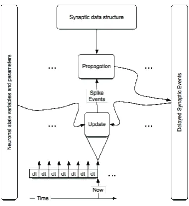
[image:65.595.202.394.484.694.2]

In a synchronous (clock driven) system model state variable updates (update phase) and spike communication (propagation phase) are accomplished with every integration step (Figure 3.1-1). The integration step is constant.

(66)

The order of computation for this type of systems per second of simulation time is defined by the following equation [1]:

(3.1-1)

where is network size, is average firing rate, is average target neurons per spike source.

Dominating phase (update or propagation) is determined by complexity of a neuron model, density of synaptic connections and complexity of the algorithm responsible for handling delays. For this type of systems delays can be effectively managed by circular buffers: fixed time resolution determines both update and propagation delay time steps.

(67)

Figure 3.1-2 Delays and cancellations due to quantization error in a synchronous system [1]

(68)

[image:68.595.107.492.131.474.2]

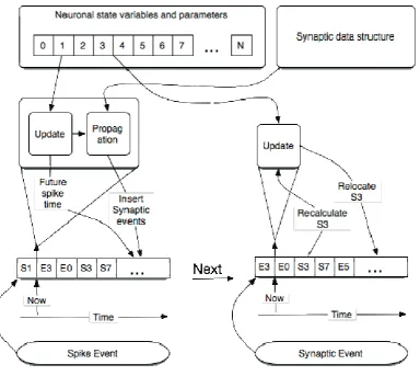
Figure 3.1-3 Asynchronous system: simulation execution flow

Computation order for asynchronous system per second of simulation time is stipulated by the following formulae [1]:

(3.1-2)

(69)

more than that of propagation operation in (3.1-1), because it includes update and propagate execution times. Besides, if implemented in software, data structure handling (insert, extract, sort, shift etc) is a crucial component of such an operation and may result in memory bounded implementations. This handling can be somewhat reduced if transmission delays are guaranteed to be more than certain value. Indeed, in this case all events within this time starting from the current time are certified not to be changed.

The benefit and, at the same time, the drawback of asynchronous system is independence of its time flow from , which requires explicit solutions for neuron model differential equations in order to calculate model variable value at any time. However, if such solutions do not exist, event-driven updates of the state variables can result in accuracy degradation due to sparsely spaced in time evaluations of state variables if future spike times do not exist. Nevertheless, this depends on numerical integration method chosen (discussed further) as well as how it is applied within the system. Conversely, the accuracy of asynchronous system outperforms that of synchronous system, because of precise event timing, if there are enough model variable updates per unit time for all neurons in the network. In the latter case and with software implementations this accuracy can be as high as the precision of data types used (single precision FP, double precision FP, etc). This is important for systems targeting implementation of high-accurate biological mechanisms, such as STDP (see section 2.1.3).

(70)

[image:70.595.183.417.123.367.2]

Figure 3.1-4 Dynamics in neuronal systems with STDP: impact of the simulation strategy (clock-driven: cd; event-(clock-driven: ed) on the facilitation and depression of synapses [1]

Event-driven systems have computational advantage in speed due to applying computation only at the time of the event. However, this advantage may be circumvented in parallel implementation by the fact that event-driven system serializes spike events in respect to time, which prohibits processing their target synapses in parallel. For example, if in a case of synchronous system two synaptic events are scheduled to execute at the same integration step, then in a case of asynchronous system even a slight deviation in time of these events results in serialization of their processing.

(71)

[image:71.595.177.419.278.544.2]

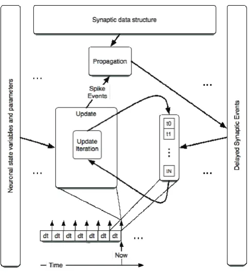
A hybrid system (Figure 3.1-5) is a merged clock-and-event driven system. In this type of system state variable updates and spike communication are done with every integration step. However, time precision of spike and synaptic events is not limited by the time grid. Instead, events are recorded in the queue following the principle of asynchronous system. The size of time step is determined by the number of updates per unit of simulation time