Evaluation of two applications of spectral mixing models to image fusion

Rochester Institute of Technology

RIT Scholar Works

Theses

Thesis/Dissertation Collections

8-11-1997

Evaluation of two applications of spectral mixing

models to image fusion

Gary Robinson

Follow this and additional works at:

http://scholarworks.rit.edu/theses

This Thesis is brought to you for free and open access by the Thesis/Dissertation Collections at RIT Scholar Works. It has been accepted for inclusion

in Theses by an authorized administrator of RIT Scholar Works. For more information, please contact

[email protected]

.

Recommended Citation

EVALUATION OF TWO APPLICATIONS OF SPECTRAL

MIXING MODELS TO IMAGE FUSION

by

Gary D. Robinson

Captain, USAF

A thesis submitted in partial fulfillment of the

requirements for the degree of Master of Science

in the Center for Imaging Science,

Rochester Institute of Technology

August 1997

Signature of

Author

G_a--=ry_D_"R_o_b_i_ns_o_n

_

Accepted

by

H_e_n--<..ry_E_"_Rh_o_d--<..y

f...;,.~_,(_)_9_f

_ _

CHESTERF.CARLSON

CENTER FOR IMAGING SCIENCE

COLLEGE OF SCIENCE

ROCHESTER INSTITUTE OF TECHNOLOGY

ROCHESTER, NEW YORK

CERTIFICATE OF APPROVAL

M.S. DEGREE THESIS

The M.S. Degree Thesis of Gary D. Robinson

has been examined and approved by the

thesis committee as satisfactory for the

thesis requirement for the Master of Science Degree

Dr. John R Schott, Thesis Advisor

Dr. Robert Fiete

Rolando Raqueno

TIlESIS RELEASE PERMISSION

ROCHESTER INSTITUTE OF TECHNOLOGY

COLLEGE OF SCIENCE

CHESTER F. CARLSON CENTER FOR IMAGING SCIENCE

Title of Thesis:

Evaluation of Two Applications of Spectral Mixing Models to Image Fusion

I Gary D. Robinson, hereby grant permission to the Wallace Memorial Library ofR.I.T. to reproduce my thesis

in whole or in part. Any reproduction will not be for commercial use or profit.

Signature:

--;-

_

---'~'4C--',~:L.7_6~7--Acknowledgments

Iwantto thankallthemembersof_mythesiscommitteeforthe

help

and guidance

they

provided

during

thecourse ofthisresearch. Aspecific acknowledgment goesto_mythesis advisor,Dr. John Schott for

helping

to

answerquestionsand_{for providing ideas for different}avenues ofinvestigation.

Iwould alsoliketothank theDIRSstaff and students. Thestaffkeptthecomputers_runningand

provided me with valued assistance withDIRSIG.

My

fellowstudentstook time tolistento_myresearch difficultiesand offersuggestions,manyof which provided successful alternativesformyresearch.

Table

of

Contents

1.INTRODUCTION 1

1.1 SpatialvsSpectral Resolution 1

1.2 Correlation 2

1.3 Mixed Pixels 3

1.4 Scale Factor 4

1.5 Obtaining High Resolution MaterialMaps 5

1.6 Outline 7

2. BACKGROUND AND LITERATURE REVIEW 9

2.1 Existing Image Fusion Methods 9

2.1.1 Image

Mergingfor Enhancement of Visual

Display

10

2.1.2 Image

Merging

by

Separate_{Manipulation of Spatial Information} 11

2.1.3Image

Merging

Which Maintains Radiometric

Fidelity

12

2.2 Spectral Unmixing Methods 19

2.2.1 Tricorder 20

2.2.2 Spectral Mixture Analysis (Traditional

Unmixing)

23

2.2.3 Constraint Conditions 27

2.3 Image Fusion Via Stepwise UnmixingandSharpening 29

2.3.1 Stepwise

Unmixing

30

2.3.2Constraints 33

2.3.3

Sharpening

35

3. APPROACH 39

3.1 UseofSynthetic Imagery

(SIG)

39

3.2 Test Method Overview 40

3.3 SelectionofTestImages 42

3.4 CreationofPanchromatic Data Sets 50

3.5 Generating Fraction Maps 51

3.6 Endmember Selection 52

3.6.1 Maximum Noise Fraction

(MNF)

Transform 53

3.6.2 Pixel

Purity

Index 54

3.7 Obtaining Sharpening Library 61

3.8Error Metrics 63

3.8.1 Squared Error 63

3.8.2 Effective RMS 64

3.8.3 Effective Edge RMS 64

3.9 Generating Output Images 65

3.9.1 Fusion 65

3.9.2

Unmixing

68

3.9.3

Sharpening

76

4.RESULTS 82

4.1 PCvsUNIX 82

4.2 CPUTIME 82

4.4EffectsofScale 86

4.5NumberofEndmembers 89

4.6 EffectsofShadow 91

4.7 VisualEvaluation 103

5.CONCLUSIONS AND RECOMMENDATIONS 113

5.1ConclusionsBasedonQuantitativeData

(Truth)

113

5.2ConclusionsBasedonQualitativeData

(Visual)

114

5.3 ProposedRevisiontoSquared Error Metric 114

5.4 Recommendations 115

5.4.1 AlgorithmImprovements 116

APPENDIXA: SOLVINGTHE LSE PROBLEM 120

APPENDIX B: SOLVINGTHE LSI PROBLEM 122

APPENDIX C: DATASETS 126

LIST

OF

FIGURES

Figure 1: SpectralBandpassesofTMandSPOT Pan Bands 2

Figure2: BasicMdcture Types 4

Figure3: IllustrationofSuperpixels andSubpixels 5

Figure4: UnmixandSharpen Image Fusion Process 6

Figure5: SharpenandUnmdcImage Fusion Process 7

Figure6: Example Look-Up Table 15

Figure7: Possible Superpixel NeighborhoodsinExtended Regression Method 17

Figure8: Sample Spectra Using Tricorder Algorithm (Clarketal,

1990)

21

Figure9: ThreeMaterialMdcturesinTwoSpectralBands 28

Figure 10: Mixture Requiring Negative Fractions 28

Figure 11: IllustrationofSharpening 35

Figure 12: Test Plan Overview 41

Figure13: Forest Test Scene (Color

Image)

44

Figure 14: Rochester DIRSIG Scene (Color

Image)

46

Figure 15: Band4 (570- 650

nm) ofDAEDALUS Image 47

Figure 16: Band 15 (749

-760 nm)ofHYDICEImage 48

Figure 17: Perfectly Unmixed MaterialMapsfor

Grass, Dirt,

& Deciduous 52

Figure 18: Perfectly Unmixed MaterialMapsfor

Grass, Water,

Roof

Gravel, Loam,

Trees 52

Figure 19: Locating Extremain thePixel Purity Index 54

Figure20: ObtainingEndmembersfromPPI Clusters 55

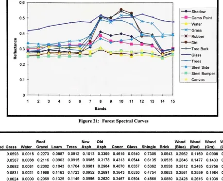
Figure21: Forest Spectral Curves 57

Figure22: Rochester Spectral Curves 58

Figure23: DADEALUS Spectral Curves 59

Figure24: HYDICE Spectral Curves 61

Figure25: SpectralCurvesforSharpening Bands

(HYDICE)

62

Figure26: ComparisonofOutputfromSimple RatioandGlobal Regression Methods 66

Figure27: FusionProgram Flow Diagram 67

Figure28: Sample Fusion Header 68

Figure29: Stepwise Unmixing Program Flow Diagram 70

Figure30: TraditionalUnmixing Program Flow Diagram 71

Figure31: Sample Unmixing Header 72

Figure 32: Sharpening Program Flow Diagram 77

Figure33: Sample Sharpening Header 78

Figure34: Squared ErrorandRun Times (Forest

Scene)

83

Figure35: RMS ErrorsforFusionofForest Image 84

Figure36: RMS ErrorsforFusionofDAEDALUSImage 85

Figure37: RMSErrorsforFusionofRochesterImage 86

Figure 38: Unmixing Forest SceneatVariousResolutions 87

Figure39: Unmixing Rochester SceneatVariousResolutions 87

Figure40: Image EnhancementforForest SceneatVariousScale Factors 88

Figure41: Image EnhancementforRochesterSceneatVariousScaleFactors 89

Figure42: ResultsofTraditionalUnmixingforRochesterScenewithVariousNumbersof

Endmembers 90

Figure44: EffectofShadow Endmember

(FuseAJnmdc)

93

Figure45: EffectofShadow Endmember(TraditionalUnmix/Sharpen) 93

Figure46: KeytoForest Scene Fraction Maps 94

Figure 47: Forest Scene Fraction Maps (Stepwise

Unmix/Sharpen)

Without Shadow Endmember...95

Figure 48: Forest Scene Fraction Maps (Stepwise

Unmix/Sharpen)

With Shadow Endmember 96

Figure49: Forest Scene Fraction Maps

(TraditionalUnmix/Sharpen)

Without 97

Figure50: Forest Scene Fraction Maps

(TraditionalUnmix/Sharpen)

With 98

Figure 5 1: Forest SceneFraction Maps (Fuse/Unmix

Method)

Without Shadow Endmember 99

Figure 52: Forest Scene Fraction Maps (Fuse/Unmix

Method)

With Shadow Endmember 1 00

Figure 53: Forest Scene Truth Fraction Maps

(4X)

101

Figure 54: Error CalculatedfromShadow ClassMapvsErrorCalculatedfromClass Map

Without Shadow (oneof_two) 102

Figure 55: Error CalculatedfromShadow ClassMap vsErrorCalculatedfromClass Map

Without Shadow (twooftwo) 103

Figure56: KeytoDAEDALUS Scene Fraction Maps 104

Figure57: Fraction MapsforDAEDALUSImage (Stepwise

Unmix/Sharpen)

104 Figure58: Fraction MapsforDAEDALUSImage

(TraditionalUnmix/Sharpen)

104

Figure59: Fraction MapsforDAEDALUSImage

(Fuse/Unmix)

105

Figure60: Fraction MapsforDAEDALUS Image (Degradedto

4X)

105

Figure61: KeytoRochesterScene Fraction Maps 106

Figure62: Fraction MapsforRochester Scene

(Fuse/Unmix)

106

Figure63: Fraction MapsforRochesterScene

(Stepwise/Sharpen)

107

Figure64: Fraction MapsforRochester Scene

(Traditional/Sharpen)

107

Figure65: Rochester Scene Truth Fraction Maps

(4X)

108

Figure66: KeytoHYDICE Scene Fraction Maps 109

Figure67: Fraction MapsforHYDICE Image

(Stepwise/Sharpen)

Using One Sharpening Band 109

Figure68: Fraction MapsforHYDICEImage

(Stepwise/Sharpen)

Using 110

Figure69: Fraction MapsforHYDICEImage

(Traditional/Sharpen)

Using 110 Figure 70: Fraction MapsforHYDICE Image

(Traditional/Sharpen)

Using 1 11

Figure71: Fraction MapsforHYDICE Image

(Fuse/Unmix)

112

Figure 72: Fraction MapsforHYDICE Image (Degradedto

2X)

112

LIST

OF TABLES

Table1: Basic ANOVATable 31

Table2:Extra SumOfSquaresANOVA Table 32

Table3: Necessary ConditionstoMinimizeL 37

Table4: M-7

(Forest)

Spectral Bands

(jxm)

42

Table5: M-7

(Rochester)

Spectral Bands

(um)

45

Table6: DAEDALUS SpectralBands

(u.m)

48

Table7: HYDICESpectral Bands

(nm)

49

Table 8: Forest Spectral Library 56

Table 9: RochesterSpectral Library 57

Table 10: DAEDALUS SpectralLibrary

(p.m)

58

Table11: HYDICE Spectral Bands

(nm)

61

Table 12: SpectralLibraryforSharpening Band

(Forest)

62

Table13: SpectralLibraryforSharpening Band

(Rochester)

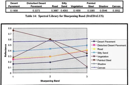
62

Table 14: SpectralLibraryforSharpening Band

(DAEDALUS)

62

Table 15: SpectralLibraryforSharpeningBands

(HYDICE)

63

Table16: DataforForestScene With Shadow Endmember (Uncorrectedfor

Shadow)

126 Table 17: DataforForest Scene With Shadow Endmember (Correctedfor

Shadow)

127

Table 18: DataforForest Scene Without ShadowEndmember 128

Table 19: DataforDAEDALUSscene 129

ACRONYMS LIST

ANOVA AVIRIS DC DIRS DIRSIG ERDvl GIFOV HPF HRP HRXS HYDICE IDL IHS LDP LRXS LSE LSI LUT um MNF MRI MS MSE MSR MSS NIR nm NNLS PC PCA PPI RBV RMS RSI SE SIG SIR-A SPOT SS SSE SSR SWIR TM VIS

AnalysisofVariance

Airborne Visible/Infrared

Imaging

Spectrometer

Digital Count

Digital Image

Processing

andRemote

Sensing

Digital Image

Processing

andRemote

Sensing

Synthetic Image Generation

EnvironmentalResearch InstituteofMichigan

GroundInstantaneous FieldofView

High Pass Filter

HighResolutionPanchromatic

High Resolution Multispectral

HyperspectralDigital

Imagery

CollectionExperiment

InteractiveData Language

Intensity

Hue Saturation Least Distance

Programming

Low Resolution Multispectral Least Squares

Equality

LeastSquares

Inequality

Look-up

Table Microns (10"6

meter)

Maximum Noise Fraction

Magnetic Resonance

Imaging

Mean Square

Mean Square

(Error/Residual)

Mean Square

(Regression)

Multispectral Scanner

Near Infrared (Regionof

Spectrum)

nanometers(10"9_meter)

Non-NegativeLeastSquares

PersonalComputer

PrincipalComponents Analysis

Pixel

Purity

Index

Return Beam Vidicon

Root Mean Square

ResearchSystemsIncorporated

SquaredError

SyntheticImageGeneration

Shuttle

Imaging

Radar

SystemePour1'

Observationdella Terre

SumofSquares

SumofSquares

(Error/Residual)

SumofSquares

(Regression)

Short WaveInfrared(Regionof

Spectrum)

Thematic Mapper

[image:11.552.89.449.126.653.2]

1.

INTRODUCTION

1.1

Spatial

vs

Spectral Resolution

Remote sensing instrumentsare capable ofobtaining imageswithhighspatialresolution,orhigh

spectral resolution. Spatialresolution referstohowwella sensor can resolvethespatialdetailsof a scene. Itis

often measured

by

thesensor'sGround Instantaneous FieldofView (GIFOV). The GIFOV istheprojection of

thedetectoraperture, through thesensor'soptics,ontotheground. AsmallerGIFOVreferstoa sensor with

higherspatial resolution. AsmallGIFOVcanbeobtained

by

_usinga smalldetector.

However,

inorderto

obtaina sufficient number of photonsforuseful

imaging,

andtomaintain an adequate signaltonoise

level,

the

detectormustbesensitive over a_relativelywide spectralband. Spectralresolution refersto thewidth ofthe

bandpasswhere radianceismeasured; thenarrower

(finer)

thespectralresolution,themorebandsthatcanbe

obtained over a specificspectral range. Toobtainhighspectralresolution,a narrowfilteror_{grating is}addedto

thedetector. Inordertoobtain sufficient photonsthedetectormustbe

large,

leading

toalarge GIFOVandlow

spatial resolution. Twotypesof remote_sensingplatforms are_commonlyused. Onetypecreateshighspatial

resolutionpanchromaticimages

(typically

inthevisible or nearinfraredregion of_{the spectrum),}andtheother

typecreates multispectral orhyperspectral imageswithfinespectral resolution.

Therewillalwaysbesometrade-offbetweenspatial and spectral resolution. Imageswithhighspatial

resolutioncanlocateobjects withhighaccuracy,whereasimageswithhighspectral resolution canbeusedto

identify

materials. With differentsensors_collectinginformationoverthesame_area,itisusefultomergethe

dataintoahybridproduct_containingtheusefulinformationofbothplatforms. Suchahybrid imagewithhigh

1.2

Correlation

Generating

hybrid imagesrequiresalargeamountof correlationinimages. ConsidertheLANDS AT

ThematicMapper

(TM)

whichhassix spectralbandsinthereflective region_{ranging from 0.400}umto2.350

um,andtheFrench SPOTpanchromaticbandwhich rangesfrom 0.5 10umto0.730um. Asshownin Figure

1,

thereisspectral_overlapbetween SPOTandTMbands2and

3,

andthedigitalcountsinthe_overlapregion will

be

highly

correlated. Hybridimagesofthesebandswill show

definite,

accurateimprovementsoverboth

originalinput images.

However,

fusing

SPOTwiththeinfraredbands (e.g. 5&

7)

willbe lessstraightforward.

Fusionofthese_poorlycorrelatedbandsrequires predictive modelstoestimatethehigh-resolution data.

TM7

MM

TM5

1

TM4

SPOT Fan

1

TM3

1

TM2

TM1

I

1 1 1 1

0.5 1 1.5

Wavelength

(um)

[image:13.552.132.427.292.518.2]

2.5

Figure 1: Spectral BandpassesofTMandSPOT Pan Bands

Mostmultispectralsensorshave bandswhosebandpassesrangethroughseveral regions ofthe

spectrum,

including

thevisible

(VIS),

nearinfrared

(NIR),

and short waveinfrared(SWIR). Atypical

panchromatic sensor will cover a much shorterportion,restrictionitselfto theVISor_{NIR (for example)}

differentmethodsfor_{performing fusion (discussed in}thenextchapter)have varying levelsof effectiveness.

Somelevelof_optimizingtoobtainthebestestimatewillalwaysbe involved.

1.3 Mixed Pixels

Theregion ontheground represented

by

one pixelinan _{image may}contain a number of materials.

The definitionofthematerialsdependsonthespecific

imaging

application. Forexample,ifoneis

looking

for

broadclassifications,pixels_{may be}classifiedas

forest,

urban,or waterand,except_{along borders between}

regions,most pixels canbeconsidered100% "pure".

However,

iftheapplicationismorespecific,thesame

pixels canbeconsidered mixtures ofdeciduousvs coniferousvegetation,or residential vscommercial,or clear

vs_siltywater. Sothedeterminationof whether a pixelismixed or pure oftendependsuponthespecific

application.

It is helpfultodividemixtures of materialsintothreescenarios. Consider firsta situation wherethere

arelinearinteractions betweenthematerialsandincidentphotons. Distinctmaterials_{may be}mixed at various

spatial scales. Amixtureis definedas aggregateifmaterials are combined atthemacroscopic scale. Thetotal

radiance

leaving

thesceneisa spatial average oftheindividualmaterials,

however,

theindividualmaterials

cannot_{be spatially}separated

by

thesensor. Anareal mixtureisalsocharacterized

by

linear

interactions,

but

involvessituations whereindividualmaterials canberesolved

by

the

(typically

high-resolution)

sensor.

Thethirdmixtureinvolvesmaterials combined atthemicroscopiclevel. Thisintrinsicmixture

involvesmultipleinteractions betweenmaterialsandincidentphotons. Theaverage radiance_typicallydepends

ona complex combination oftheindividualmaterial properties. Suchmixtures require non-linear models and

. .,,:... . :..

Intrinsic

Aggregate

Areal

1.4 Scale Factor

Figure 2: Basic Mixture Types

Hybridimagescanbeproduced

by fusing

low-resolutionmultispectralimageswithhigh-resolution

panchromaticimages. Thepixelsofthelow-resolutionmultispectralimage

(LRXS),

oftencalledsuperpixels,

coverlargerareas ofthegroundand correspondtoseveralpixels,often calledsubpixels,ofthehigh-resolution

panchromaticimage

(HRP)

asillustrated in Figure 3. Ifthe twoimages_{have been properly}registered, theneach

LRXSsuperpixel correspondstoa collection ofHRPsubpixels equivalentinsizeto thelarger low-resolution

LowResolution

Multispectral

Superpixel

High Resolution

Panchromatic

Subpixels

Figure3: IllustrationofSuperpixelsandSubpixels

ThescalefactorofthefusionreferstothedifferenceintheGIFOV betweentheLRXSandHRP

images. Forexample,considerthecasewheretheGIFOVoftheLRXS is 30mandthatoftheHRP is 10m.

Thenthescalefactor is definedtobe

GIFOV LRXS 30

Scale Factor = = ₌₃

GIFOVHRP 10

Eq. 1

Suchafusionscenariowill produce ahybridimagewith a3-times

(3X)

improvementin GIFOV. This hybrid

imagecanthenbeusedtocreatedetailedmaterial maps.

1.5

Obtaining

High Resolution Material

Maps

Therearetwostepsincreatingthedetailedmaterialmaps_previouslymentioned.

First,

the

multispectral(or

hyperspectral)

imageisusedto

identify

thematerialsinthescene. Thisprocess,often referred

specific material withinthescene.

Second,

thematerial maps andthepanchromaticimageofthesame area

serve as_{constraining inputs}toproduce sharpened materialmaps,resulting in high-resolutionmaterial maps.

Onemethod ofimagefusionusestheunmixandthensharpen procedure(See Figure 4). Analternate

method,

theoretically

_{producing identical}results,utilizesa sharpen and unmix process. _{The sharpening}

produces ahigh-resolutionmultispectralimagewhichisthenunmixedintohigh-resolutionmaterial maps. There

is littlepublished work ofimage_{fusion using}a sharpen and unmix process(See Figure5).

However,

thereare

severalapplications which utilize_sharpeningwithoutfurther processing

(unmixing)

ofthehigh-resolution

multispectral images.

1 1 1 1

J

Low Resolution

ImageCube Low Resolution

V*

U.

High Resolution

Unmix Material Maps

X

"^

if

f

Panchromatic

Sharpen Image

i

w 144

J

High Resolution Material Maps

Low Resolution

4^

w

Image Cube

Sharpen

High Resolution

Panchromatic Image

HighResolution

Image Cube

144

1

Unmix

High Resolution

Material Maps

Figure5: SharpenandUnmixImageFusion Process

1.6 Outline

Thisresearchimplemented image fusionvia a sharpen and unmix process and comparedthe_resulting

high-resolutionmaterialmapstothoseobtained viaan unmix and sharpen process. Theunmix and sharpen

process employedtwomethods_{for producing}thelow-resolutionmaterial maps. _{A recently}developedadaptive

unmixingalgorithmwas comparedtotraditional_unmixingmethods.

Sharpening

was performed onthe

low-resolution material maps produced

by

the twounmixing algorithms,andthe_resultinghigh-resolutionmaterial

maps were comparedto thosegeneratedviathesharpenand unmix process. Allmethods were evaluatedfor

Thisdocumentisorganized asfollows. Sectiontwoprovidesbackgroundreference on variousimage

fusiontechniques. Thespecific methods usedinthisresearcharediscussedinsomedetail. Sectionthree

provides an overview of_{the test method,}

including

detailson stepsinvolved intheimageenhancement methods.

Thequantitative and subjective results ofthe testsaredetailedin sectionfour. Theresults showthat the

sharpen/unmix method produces more errorthan_unmixingwiththeadaptive algorithm andthensharpening.

Fractionmaps created

by

thesharpen/unmix method are more_visuallyacceptable,containingmore

high-frequency

informationthanfractionmapsproduced

by

theunmix/sharpenmethods. Thefinalsectionindicates

2. BACKGROUND AND

LITERATURE

REVIEW

Image fusion involves_{combining different images}intoa newhybrid image. Theoriginal_{images may}

beproducts ofdifferentremote_sensingplatforms,and_{may have different}spectral and spatial resolutions. For

example,we might wishtomergedataobtainedfromtheLandsat Thematic Mapper

(TM)

withthatobtained

fromtheFrenchSystemePourl'ObservationdellaTerre (SPOT). The TM hasseven spectralbands ranging

from.45to2.35microns. Sixofthebands (1-5and

7)

have 30meter spatial resolution. Theseventhband

(band

6)

providesthermalinformationandhas 120meterspatial resolution. SPOT has 3spectralbands inthe

visible and nearinfraredregion with20meter spatial resolution. Italsohasa panchromaticbandwith 10meter

spatial resolution. Themost efficient methodforan analysttoexamine

imagery

fromthese twoplatforms would

betocombinetheusefulinformation frombothintoa singleimage.

Landsat TMandSPOTare notthe_onlytypesofdatathatcanbemerged.

Daily

et al.

(1979)

and

Chavezet al.

(1983)

merged airborne andShuttle

Imaging

Radar

(SIR-A)

imageswithLandsat Multispectral

Scanner (MSS). LauerandTodd

(1981)

combined

imagery

from Landsat MSSwithdata fromtheReturn Beam

Vidicon (RBV). Thenextgeneration ofhyperspectralspace-based sensors_{is currently in}thedesignphase.

Thesesensors willhave highspectralresolution,but verypoorspatial resolution. _{The pending increase in}

sensors willincreasetheneedfor better image fusionapplications.

2.1

Existing

Image Fusion Methods

Thereare several_existingmethodstoperformimage fusion. Munechika

(1990)

groupsthesemethods

intothreeclasses. The firstclassiscalled

"Merging

Images for EnhancementofVisual Display". These

algorithms are_primarilyconcerned with_optimizinganimage

display

sothatit looksgoodfortheanalyst. The

mergedata

by

separatemanipulation ofthespectral and spatialinformation. The finalclassiscalled"Image

Merging

toMaintainRadiometric Fidelity". Thesealgorithmsmerge

data,

whileensuringthattheradiometric

accuracyoftheoriginal multispectraldata ismaintained or_{degraded only}minimally.

2.1.1

Image

Merging

for Enhancement

of

Visual

Display

Imagefusionroutinesthatenhance visual

display

havealsobeenreferredtoas adhocmethods. The

primaryconcernistooptimizethe

display

foranalysis purposes. Thereisno concern_{in preserving}the

radiometric_accuracyofthemultispectraldata. Onemethod usedemployshistogramspecification and contrast

stretching. Twoexamples of generic methods are given

by

theequations(Welch&Ehlers,

1987)

XSJ

=a:X

^XS,

X

P

+

b,

Eq. 2

or

XS|

=

a,

x

(v^XS;

w2P)

+

b:

Eq. 3

where

XS;

isthedigitalcount

(DC)

fora pixelinthei bandofthehigh-resolution hybrid

image, XS;

isthe

digitalcountforthe_{corresponding}pixelintheoriginal multispectral

image,

P isthedigitalcountforthe

correspondingpixelinthehigh-resolutionpanchromatic

image,

w,andw2are_weighting

factors,

and_a;and

b:

are_{scaling factors}tooptimizethehybrid imageforthedynamicrangeofthe

display

system, and isan

operatorwhichcouldbeaddition, subtraction, multiplication,ratio,etc.

Asimpler adhoctechniquetoenhance aRGB

display

istoreplacethegreen channel withthe

panchromatic

data,

leaving

theredandbluechannels unchanged. Sincethehumanvisual systemismost

2.1.2 Image

Merging by

Separate

Manipulation

of

Spatial Information

Animagecanbeassumedtocontain alow

frequency

andhigh

frequency

component. The low

frequency

datacontainsthespectral

information,

whilethehigh

frequency

datacontainsthespatialinformation.

Theimage fusionalgorithmsinthisclass manipulatethespatial(high

frequency)

component while_preserving thespectral componenttogenerate enhancedimages. Braun

(1992)

comparedthreealgorithms ofthisclass.

2.1.2.1

Intensity

Hue Saturation

(IHS)

The IHStechnique_(Chavez,

1991)

canbeappliedto threebandsof multispectraldata. Three

multispectralbandsaretreatedas colors(e.g.red, green,blue). The RGBmultispectralimage istransformed to an_intensity,

hue,

saturationspace,wherethe

intensity

isassumedtocontain mostofthespatial

information,

and thehueand saturation are assumedtocontain most ofthespectralinformation. Thepanchromatic image isthen

substitutedforthe

intensity

ofthemultispectral

image,

and aninversetransformationisperformedtoreturnthe

imagetoaRGBformat. Theresultisahigh-resolution imagewhose spatial contentis derived fromthe

panchromatic

image,

and whose color

(spectral)

contentis derived fromtheoriginal multispectraldata.

Thistechniqueis basedontheassumptionthatedgeinformation

(essentially

thespatialcontent) is

contained withintheintensity. The IHStransformationworks as

long

asthepanchromaticimage is

highly

correlated withthebandsofthemultispectralimage.

2.1.2.2

Principal

Components Analysis

(PCA)

The PCAtechnique

(Chavez, 1991)

involvescalculatingtheprincipal component ofthemultispectral

image. Thiscalculation utilizeslinearalgebra,andtransformsa vector of correlateddata intoorthogonal

similarto thepanchromaticimage. The firstprincipal componentimage isreplaced

by

thehigh-resolution

panchromaticimage. All_remainingprincipal components are assumedtocontainthespectral components and

are untouched. Aninverseprincipalcomponentisthenperformedtoobtain a newhybrid image.

2.1.2.3 High

Pass

Filter

(HPF)

Thehighpassfiltertechnique

(Schowengerdt, 1980)

is basedonthe_theorythatanimage iscomposed

of ahighpass filtered imageand alowpass filtered image. The hybrid imagecanbeconstructed

by

_usingthe

high-resolution imagetoreplacethe_missingedgeinformation inthe_{low-resolution image using}theequation

HRXSj

=

LRXSj

+KJHPAN

Eq. 4

where

HRXSj

isthedigitalcount of a pixelinthej"1bandofthehybridmultispectral

image,

LRXSj

isthedigital

count ofthe_{corresponding}pixelinthej*bandofthelow-resolutionmultispectral

image,

Kj

isa constant

designedtocontrolthecontrastofthehybrid

image,

and

HPAN

isthedigitalcount ofthe_{corresponding}pixel in

thehigh-resolutionbandusedfortheedge details.

Kj

ischosen_{appropriately}toensurethat thecontrastinthe

hybrid bands isweighted_equally

by

thelow-resolutionandhigh-resolution images.

2.1.3

Image

Merging

Which

Maintains

Radiometric

Fidelity

Allofthepreviouslymentionedimagefusionmethods_primarilyenhance visualdisplay. Thespatial

resolutionofthehybridmultispectralimage improvescomparedto theoriginal multispectralimage.

However,

theexactradiometricvaluesofthemultispectralimageare oftenlost intheprocess.

Any

algorithm usedto

identify

materialsina multispectralimagerelies

inherently

onthe_accuracyoftheradiometric values withinthat

image. Inordertoexploittheinformation inthehybrid images

by

use of an automatedroutine, the_radiometry

ofthehybrid imagemust matchas_closelyas possiblethe_radiometryoftheoriginalmultispectralimage. The

2.1.3.1

Ratio Methods

Theratio methods are simpleimagefusion techniquesdesignedtomaintain_{the radiometry}ofthe

originalimage.

They

requirethat thepanchromatic_sharpeningimage be

highly

correlatedwiththemultispectral

image. Theprocedurebegins

by

dividing

thepixelsofthemultispectralimageintosubpixelswhichare equalin

sizetothepixels ofthehigh-resolutionpanchromaticimage.

2.1.3.1.1 Pradines'

Method

Pradines

(1986)

usesthe

following

equationtomergeSPOTspectralbandswiththeSPOT

panchromaticband:

HRP

HRXS,

-

LRXS(

_{Eq. 5}

1

2.HRP

superpixel

where

HRXS;

isthedigitalcount of a subpixelinthehigh-resolutionhybrid image inthei*

band, LRXSj

isthe

digitalcountofthe_{corresponding}subpixelin thei*bandofthemultispectral

image,

andHRP isthedigital

count ofthecorrespondingsubpixelinthehigh-resolutionpanchromaticimage.

2.1.3.1.2 Price 's Method

The disadvantageofthePradinesroutineisthatit doesnotaccountfor bandsthatare not

highly

correlated withthepanchromaticimage. Price

(1987)

proposesatwo-stageprocessfor

dealing

withbandsthat

are either_weaklyor_stronglycorrelated withthepanchromaticimage. Aratioisusedforthe_{stronglycorrelated}

bands,

which canbewrittenas

LRXS,

=

where_a;and

bj

areleastsquares regression coefficients of alinearfit inthei"1band,and

HRPS

isthedigital

count of an averaged panchromaticimagesuperpixel. Theregressioncoefficientsarefound

by

regressing

HRPS

againstLRXSj. The high-resolutionmultispectralimage

(HRXS)

isobtained

by

HRXSJ

=

a;

HRP +

bj

Eq. 7

and

LRXS,

HRXS;

= . Eq. 8

HRXSi,s

where

HRXS;

isthedigitalcount oftheestimateforthei*bandof ahigh-resolutionmultispectralimage,and

HRXSj.s

istheaverage of

HRXS;

overasuperpixel.

Braun

(1992)

reportsthatstage 1 ofthePriceroutineproduces results similarto thePradinestechnique.

ThemaindifferenceisthatPriceusesan estimateforthehigh-resolutionmultispectral

bands,

whereasPradines

simplyusesthehigh-resolutionpanchromaticimage.

Priceuses a

Look-Up

Table

(LUT)

instage2 ofhistechniquefor

dealing

with uncorrected spectral

bands. The LUT iscreated

by

_{first examining}the

HRPS

values,and_recordingthe_{corresponding digital}count

inthelow-resolutionmultispectralimage. Themeanofthesemultispectralpixelsiscalculatedandthevalueis

enteredintotheLUT. Figure6showsan example

look-up

table. ThevaluesintheLUTrelatethe

HRPS

digital

countsto themultispectraldigitalcountsintheuncorrelatedbands. Nowthehigh-resolutionestimates are

calculated_usingtheLUTvaluesfor

HRXS'

Average Pan DC

(HRPS)

DCfrom

Weakly

Correlated

MultispectralBands

(LRXSj)

Mean Low Res Multispectral DC

0 8,8,8,7,9,... 8

1 21,24,22,20,23,... 22

2 17,14,13,16,... 15

255

Figure 6: Example

Look-Up

Table

2.1.3.1.3 DIRS Method (Simple

Ratio)

Munechika

(1990)

presents a routine whichiseasiertoimplementthanPrice'smethod. Thismethodis

designedtoprovide as much radiometric_accuracyaspossible,andformsthebasis fortheExtended Ratioand

Global Coefficientmethods which willbe discussed in latersections. Thismethodisused

by

theDigital

Imagery Processing

andRemote

Sensing

(DIRS)

laboratory

atRITandisoften referredtoastheDIRS Method.

Munechika'

s methodbegins

by

pixel_replicatingand

blurring

thehigh-resolutionpanchromatic image

sothatitssubpixelsarethesame size asthepixelsofthelow-resolutionmultispectralimage. Thepanchromatic

image isregisteredto themultispectralimagetopreservethe_radiometryofthemultispectral image.

Thesimple ratiomethodisgiven

by

theequation

HRXS;

=

HRP

LRXS;

HRPS

Eq. 9

Thismethod works wellforspectralbandsthatare

highly

correlated withthepanchromaticimage. Itcan_easily

beshownthat thisequation_{is radiometrically}correct

by

HRXSs

N

LRXS;

N

.

HRPj

I

HRP-IPYQ

J= 1 _HRPS J

LRXSj

, = _i J

LRXS-i

= = HRP

N HRPc N

HRPS

which showsthattheaverage ofthedigitalcounts ofthehybrid imageover a superpixel equalsthedigitalcount

ofthe_{corresponding}pixelintheoriginal multispectralimage.

Munechika'

s methoddoesnot work well on mixedpixels,so an enhancementispresentedin

Munechikaet. al. (1993). Forthecase of a mixedpixel, theratio ofLRXS/HRPsisnotalwaysthebest. Inthis

case,adigitalcountof a panchromatic subpixeliscomparedtothemeandigitalcounts of_neighboring

superpixels. Ifthe

subpixel'

s ratioiscloserto thatof one ofthe_neighboringsuperpixelvalues, then that

superpixel's meanisusedforthe

LRXS/HRPS

ratioinequation9. Thismixed pixelisnot_necessarily

radiometricallyaccurateon average over asuperpixel,but itsquantitative performance ona subpixel case

exceedsthatofthesimple ratiomethod.

2.1.3.1.4 Extended Ratio

Thesimple ratio methoddoesnot maintain radiometric_{accuracy for weakly}correlatedbands. The

extended ratio methodis designedtodealwiththecase of poor spectral correlationbetweena given

multispectralbandandthepanchromaticband,andisusedinconjunction withthesimple ratiomethod,withthe

ratiomethodimplemented forcorrelatedbands. A liner relationship iscreatedbetweenthe_weaklycorrelated

band,thepanchromatic

band,

and_{any previously}predictedbandas

LRXSk

=

a0

+

a,

HRPS

+

a2

LRXSj

+

a3

LRXSj

+ ... Eq. ll

wherekreferstoa_weaklycorrelatedmultispectralbandandiand

j

are_stronglycorrelated,previouslypredicted

bands. Thecoefficientsa0, &\ ,etc. are obtained

by

performingaregressioninalocalizedneighborhood around

thetargetsuperpixelusingequation 1 1. See Figure 7foradiagramof possible superpixel neighborhoods. The

regressionis firstperformed_usingonlyone_{strongly correlated/previously}predictedband. Additional bandsare

Superpixelof Interest Shown

with Subpixels

.-':- _*Sps

'

.J-^.-:r

^j^' '' '"..

t-7

;ft "*

.;:^''W

>-^;

-.

^

-Superpixel Neighborhoods

UsedtoCompute Extended

RegressionCoefficients

andResidual Errors

Figure 7: Possible Superpixel Neighborhoods in Extended Regression Method

Oncetheregression equationissatisfied,thecoefficients are usedtodeterminethedigitalcount ofthe

hybrid imagesubpixels_using

HRXSk

=

a0

+

a,

HRP

+

a2

HRXS,

+

a3

HRXSj

+ Eq. 12

where

HRXSj

isthedigitalcount of ahybridsubpixelin band i

(previously

predicted_usingtheratio method).

Theadvantage oftheextendedregressionmethodisthatitallowsthehybrid imagetobepredicted

even_{for poorly}correlatedbands. Inaddition,

by

solving forthecoefficientsinalocalizedregion aroundthe

targetsuperpixel,theextended regression methodtends tousesuperpixels withthesame materialtypesasthe

targetsuperpixel. Aproblem withtheextendedregressionmodelisthatitproduces_{noisy images}when usedin

areas with uniformdigitalcounts.

Any

small changeina_{sharpening band}or errorsina_previouslypredicted

regression producesimprovedresults overthesimple ratio when usedinregions wherethereismuchbrightness

variation within a materialtype.

2.1.3.1.5 Global

Regression

Method

Theglobal regression methodisdesignedtoovercomesome ofthelimitations oftheextended

regressiontechnique. Ratherthan_performinga regressioninalocalizedwindow around a_subpixel,data from

theentireimage isused. Theassumption usedisthatthebest datatosolvetheregressionisfromsuperpixels

withthesame spectral characteristics asthetargetsubpixel.

First,

an unsupervised classifier with alarge

numberof classesisusedonthemultispectraland panchromatic images. Aclass_{map is}created with all pixels

classifiedintosome spectral class(notethatno classtypeneedstobeassignedtotheseclasses). Theregression

inequation 11 isapplied_usingpixelsthatareinthesame class asthe targetsubpixel. _{The remaining}portion of

theglobal regression routineissimilartothatfortheextended regressiontechnique,withbands

incrementally

added untiltheresiduals oftheregression equation arebelowadesired threshold. Equation 12 isemployedwith

thecoefficients obtainedfromtheregressiontoobtainthehigh-resolutionmultispectralimage.

Braun

(1992)

notesthat theglobal regressiontechnique,onaverage,outperformstheextended

regressionroutine. Theextendedregressionproducesnoisyresultsin low

frequency

areas,whereastheglobal

regressionsoftensthenoisewhilepreservingtheedges.

2.1.3.2

Algorithm

Summary

Image fusionworksbestwhenthelow-resolutionmultispectral image bandsare

highly

correlated with

the high-resolutionpanchromaticband. Whenthereisweakcorrelation,the_qualityoftheimagefusionwillbe

degraded,

and routinesthat_separatelymanipulatespatialdata may introduceradiometricinaccuracies. The

Intensity

Hue Saturationmethodis insome waystheleastrobustbecause itcan_{only be}appliedto threebands.

separatelymanipulatethespatialdata. ThePriceandMunechikamethodsproduce similar resultsinthe

correlatedbands. Thesimpleratiotechnique

by

Munechika formsthebasis fortheextended and global

regression methods. Theextendedregressionroutine worksbestwhenscenes containhigh

frequency

information,

andtheglobalregressionworksbestwhenthescene contains medium orlowfrequency.

2.2 Spectral

Unmixing

Methods

Themultispectralremote_sensingplatform_typicallyhaspoor spatial resolution. The largepixel sizes

imply

thatthe_majorityofthepixelsinthemultispectralimagewillbemixed. Applicationssuch as_mapping

vegetation or

locating

mineral resources require suchmixed pixelstobeseparatedintotheindividual

constituents(oftencalled_endmembers)whose radiances contributetothesingle mixed pixel value. Spectral

unmixingtransformsthedigitalcounts of mixed pixelsintoa series of maps which are estimates ofthe

percentageor abundance oftheindividualmaterials withina scene.

Spectral unmixing has beenused to_{map many different}materials. Images fromtheAirborne

Visible/Infrared

Imaging

Spectrometer

(AVIRIS)

wereusedtocreateindividualmaps of greenvegetation,

nonphotosyntheticvegetation,and soil(Robertsetal 1993). AVIRISdatawas also usedto_{map desert}

vegetation(Smith 1990). Hyperspectralsensors such asAVIRISare

ideally

suitedtospectral_unmixing

applicationsdueto therequirementthat therebemore spectralbandsthanconstituentstobeunmixed.

Spectral unmixingcan_{classify images using}scene-derived endmembers or reference endmembers

(reflectancespectra measured

by

fieldor

laboratory

instruments). Whenreferenceendmembersareused,

atmospheric compensationandtheresponsivityofthesensor mustbetakenintoaccount.

Twomethods of spectral_unmixingare prevalentinavailableresearchliterature. TheSpectral Mixture

AnalysisofSmithet al

(1990)

andRobertset al

(1993)

provides estimates ofthepercentages ofendmembers

employingclassical_unmixingmethods,whereastheTricordermethod ofClarketal

(1990)

producesthe

2.2.1 Tricorder

Clarketal

(1990)

employa method referredtoasTricordertodeterminetheindividualendmembers

withinthemixed pixels of amultispectralimage. Tricorder issimilartospectroscopicanalysis employed

by

scientists,and employsthesame steps usedtoanalyze a spectrum. Endmembersareidentified

by looking

for

specific absorptionfeatures. Forexample,kaoliniteanddolomitehavecharacteristic absorptionfeatureswhich

Tricordercanlocate inthespectrum ofa mixed pixel.

The

following

definitionof absorptionband depth isemployed

by

thealgorithm

D

= 1-^- _{Eq. 13}

where

Rb

isthereflectanceinthecenter of an absorption

feature,

and

Rc

isthereflectance ofthecontinuum at

thecenter ofthefeature. Thecontinuumistheshapethespectrum wouldtakeiftheabsorptionfeaturewere not

present.

Typically,

it iscreated

by

_{simplyconnecting}thewings oftheabsorptionfeaturewith a straightline.

See Figure8.

The Tricorderalgorithmrequiresthat thedata becorrectedforatmospheric effects. Green et al₍₁₉₉₃₎

present a methodtocalibrateAVIRIS data foratmospheric effects.

Assuming

thedata iscorrectedfor

atmosphere,Tricorderusesthe

following

steps.

1)

Convolvethe

library

spectra withthesensor response soit

resemblestheimage data.

2)

Converttheimage data from digitalcountstoapparent reflectance.

3)

Remove

thecontinuuminthe

library

andimagespectra_using

Lr(A)

=

^-

_{Eq. 14}

CL(A)

and

s m -

S(A)

where

Lc

isthecontinuum-removed

library

reflectancespectrum,Listhe

library

spectrum,

Sc

isthe

continuum-removed sensorspectrum,Sisthesensorspectrum,and

CL

and

Cs

arethecontinuum spectra estimatedfroma

fitthroughthewingsoftheabsorptionfeature.

REFLECTANCE 0.8 0.6 0.4 0.2 REFERENCE KAOLINITE 0.5 U z o 0.4

fe

0.3 a. 0.2 I

0.5 1.0 1.5

WAVELENGTH

(uM)

2.0 2.5

-l ₁ l l i I i ₁ 1

r-q

Reference Kaollnlte

H

AVIRIS line 404 sample 37

J

I L J U

J_

J-Continuum

Band Depth

2.1 2.2

WAVELENGTH (um)

2.3

Theabsorptionfeaturesinthereferencespectrum are_typically strongerthaninthespectrumrecorded

by

theremotesensor,sothespectralcontrast ofthereferencemustbechangedtomatchthecontrast ofthe

sensor spectrum. Thecontrastofthereferencespectrumismodified

by

Lr

+k

Lc

= = _{a +}

bLc

Eq. 16

1+k

where

Lc

isthecontrast reduced spectrumthatbestmatchesobservation,k isaconstant,and a=

k/(l+k)

_andb

= _l/(l+k).

Thecoefficients a&bmustbe determinedsuchthat_theygivethebest fitof

Lc

to theobserved

spectrum. Aleastsquarefit isperformed_using

!Sc-blLc

a =

b

=

Iii-S^l

'

and

1-b

k

= Eq. 17

b

where nisthenumberof spectral channelsinthefit. Amaterial_{map is}produced

by fitting

a reference spectrum

to thespectrumofeach pixelinahyperspectral dataset. The band depth isproportionaltotheabundance ofthe

materialandthegoodnessoffitprovides a confidencefactor.

By

plotting

D*R2,

thebrightareas willshowhigh

abundancewithhighconfidencein thederivedsolution. Amaterialistypicallycharacterized

by

morethanone

absorption

feature,

so several_{features may be}used

by

thealgorithm. _{The features may}alsobeweighted, sothat

2.2.1.1

Tricorder

Summary

Clarket al

(1990)

useAVIRIS datatodemonstratetheTricorderalgorithm,and report good success.

Thismethod can even create maps of materials with complicated absorptionfeatures (e.g.thekaolinite doublet).

Spectralmixture analysis(discussedin thenext_section)canbeaccomplished without atmospheric

compensation.

However,

theTricorderalgorithm will not work withdatathathasnotbeencorrectedfor

atmospheric effects. Anothercontrastbetweenthe twomethodsisthefactthat_unmixingwiththeTricorder

algorithm_{may only be}performedonhyperspectral

data,

whereasspectral mixture analysis canbeperformed

(withalimitednumber ofendmembers)on multispectralimages. Tricorder isalsolesssensitivetosignalto

noisein individualchannels_{because many}channels are usedto _mapan absorptionfeature. An inexperienced

usercannot_simplystart_workingand_achievingsuccessful resultsbecauseexpertknowledgeof_spectroscopy

by

theuserisrequiredforthisalgorithm. Tricorderwas notimplemented forthiswork.

2.2.2

Spectral Mixture Analysis (Traditional

Unmixing)

Spectralmixture analysisassumesthatfora multispectral

image,

thespectral variationis duetoa small

number ofendmembers. Theseendmembers allhave differentreflectance spectra andthedifferences inthe

spectra serve as

"fingerprints"

to

identify

thedifferentmaterials. Inthecase of areal and aggregate mixtures,it

ispossibletoproducealinearmixture oftheseendmembersthat_closelymatchestheobserved spectra measured

by

thesensor. For Nendmembers, thisbecomes

LSesora)

=

XLe(A)fe

_{Eq. 18}

e=1

where

Lsensor(^)

isthespectral radiance_reachingthesensor,

fe

isthefractionof endmember e withinthepixel.

and

Le(^)

isthespectral radiance ofthatendmember.

DCj

=

gj-Lj

+

bj

Eq. 19

and

Li

=

iLsensorU^.a)^

Eq. 20

where

DC,

,g;and

bj

arethedigitalcount recorded

by

the

detector,

gain ofthe

detector,

andbias forthe i"1

spectral

band,

(3j(A.)

isthedetector'sspectralresponsivity,and

Lj

istheeffective radiance"seen"

by

thesensor.

Notethat themeasured radianceisaffected

by

thespectral response ofthesensor.

Combining

equations 18and

20,

i,-Jl

,Le(A)fey3(A)dAev ' _{e '}

N j.

L,

=

2>e

JLe(A)B,(A)dA

e=_l

X

N

Li

=

2X,ife

_i = _{!--k Eq. 21}

e=₁

where

Lei

istheeffective radiance ofendmembere measuredinthef1bandofthe sensor,andk isthenumber

ofbands.

Theeffects oftheatmosphere can oftenberemoved. Greenet al

(1993)

present a method of

calibrating AVIRIS datatoeliminate atmospheric effects. When digitalcounts are correctedforatmospheric

effects,spectral mixture analysis_{may be done in}termsoftheapparent reflectance oftheendmembers

DC,

=

giR,

+b,

Ri

=

2X,i

f

Eq. 22

e=1

th

where

R.ti

istheeffective reflectanceof endmember einthei spectralband.

Spectralmixtureanalysis produces equivalent resultsifcalculations are performed intermsof radiance

Spectralmixtureanalysisisperformed_usingthe

following

equation

N

LRXS;

=

XRe,i

fe

+

i

i=l....k Eq. 23

e=1

where

LRXS,

isthedigitalcountinthei"1spectral

band, fe

istheunknownfractionof endmember einthepixel,

Rei

isthereflectanceof reference endmember einthei*band (obtained froma

library

ofendmembers), j isthe

errorin band i forthefitofNendmembers,andk isthenumber ofbands inthelow-resolution image. Spectral

mixture analysis requiresthat theleastsquaresfittoequation23be"good"

(AgoodfitoccurswhentheRMSof

the_e,values_{is approximately}thesamemagnitude asthesensor noise). Theerroris duetotheresidualvariance,

andisa measure ofthespectralvariationnot predicted

by

themodel.

ThegoalistocalculatetheNunknownfractions. Equation 23 istheavailable equation and provides a

constraint onthenumberof endmembersthatcanbeunmixed orthenumber ofbandsrequiredinthe

multispectralimage. Sothenumber of endmembers mustbek>N.

Using

LANDSAT TMas anexample, the

maximumnumberofendmembersthatcanbeunmixedis6 (k=_{6). This isa rather small number of possible}

endmembers and explainswhy hyperspectralsensorsare much more suitedto_unmixingapplicationsthan

multispectralsensors. Themultiplebandsofthehyperspectralsensor(e.g.224 bands for

AVIRIS)

areideal for

use withunmixingequations.

Smithet al

(1990)

usea_two-stepprocess wheretheimageismodeled as mixtures ofimage derived

endmembersandthentheimageendmembersaremodeled as mixtures of reference endmembers. Image

endmembersare often amixtureofothermaterials and are selected suchthata minimum number of reference

spectracombinetodescribethem. Forexample,animageendmember_{may actually be}composed of407c

vegetationand60%soilbecauseno pure pixels of vegetation or soil are presentinthescene. Inthesecond_step

oftheprocessthefractionsofthisimageendmemberwouldbeunmixedintofractionsof reference spectrafor

soil andvegetation. Imageendmembersare expressed aslinearmixtures of reference endmembersinthe same

are convolved withthebandpassofthesensorbandstoensureaccurate comparisonbetweentheimage

endmembers andthereferenceendmembers.

Smithet al

(1990)

usea shade endmembertoaccount_{for shading}and shadows. Thefractionimage

basically

reflects

lighting

and_topographyvariationsintheimage. Tocompensateforpossible anticorrelation

betweenvegetation/soilfractionsandtheshade

fractions,

allfractionsexceptshade are re-scaledtosumtounity,

pixel

by

pixel. Forexample,a vegetationendmember_{may be}scaled_using

f

Vfs

= _{Eq. 24}

(l"fshade

>

where

Vfs

isthescaled vegetation

fraction,

fvcg

istheoriginal vegetation

fraction,

and

fshade

istheshadefraction.

Thisprocessremoves_onlytheshadefraction fromthepixel. _{The scaling is}correctassumingshadeis equally

present_amongalltheendmembers. For

display

purposes,thecomplement oftheshadeimage

(l-fShade)

is

combined withthe

Vfs

imagetoproduce animagewhich matchesobserverintuition (e.g. highshadefractions

appeardark).

Iftwoor more endmembers arecloselyrelated(e.g.differenttypesofsoils),thesameprocedurefor

normalizing forshadecanbeusedtoemphasizethefractions betweenthese_closelyrelated endmembers. For

example,giventwodifferentsoilendmembers,(Saand

Sb),

a scaledfraction forsoil endmemberSacanbe

generated

by

fSa

Saf = Eq. 25

(fsa+fsb)

where

Safs

isthescaledfraction forendmemberSa. Highervalues of

Safs

indicatean abundance of soiltypea,

andlow fractions indicatemore of soiltypeb. Thisprocess canbeused with equation22toproducefraction

2.2.3 Constraint

Conditions

Thepreviousdiscussionpresentedspectral mixture analysis as an unconstrained problem.

However,

theliteraturecontainsthreedifferentconstraint conditions. Thefirst isunconstrained,as_previouslypresented,

where_{fractions may}assume whatever valueisneededtoproduce an estimate with minimum error. Thesecond

conditioniscalled_partiallyconstrained.

Here,

thesum of allthefractionswithin a pixel mustbeunity.

N

2X

=

1

_{Eq. 26}

e=1

providingone_equalityconstraint. Positiveand negative_{fractions may be}generated

by

bothunconstrained and

partiallyconstrained unmixing. The

fidly

constrainedconditionleviestheadditional requirementthatall

individualfractions lie betweenzero andone.

fe

=

1,

(0<fe<l)

_{Eq. 27}

e=1

providing 2*N

inequality

constraints.

Althoughthe

fully

constrained situation seemstobethebestmethodbecause itmatches

intuition,

the

negativefractionsreturned

by

the_partiallyconstrained casedo havephysical explanations. The

following

example_{may illustrate}thispoint. Figure9 illustratesmixtures ofthreematerialsintwospectralbands. The

reflectanceineachbandisplotted_alongtheaxes. Thevertices ofthetrianglearelocatedatthereflectance of

purepixels ofthe threematerials. Mixturesofthe threematerials with positivefractions are_{located along}and

withintheperimeter ofthe triangle. Forexample,a50/50mixture of materials 1 and2materials_{lies midway}

"

Band 2

Band

1

Figure9: Three Material Mixtures in Two Spectral Bands

Figure 10 illustratestheresultsduetorandomvariation. Althoughendmembers are plotted as specific

points,they trulyrepresentthemean vectors. Ifthereal materials are gaussiandistributedaboutthe mean, then

thecontours plottedin Figure 10represent_equally

likely

departures fromthemean values.

Band 2

Band 1

Supposea particular pixel contains endmembers whose reflectance values are represented

by

thevertices ofthe

solidtriangle. Thepossible mixturesforthispixelliewithinthesolidtriangle. Notethat thepointdenoted

by

"X"

lieswithinthesolidtrianglebutoutsidethe triangleformed

by

thereference endmembers. Themixtureisa validone,butrequires negativefractions

involving

thereference endmembers.

2.2.3.1 Spectral Mixture Analysis

Summary

Smithet al

(1990)

useLandsat TM dataforspectral mixture analysis. _{The relatively}small number of

bandsdoesnot allow unique spectralidentifications.

Many

materials,measuredthroughtheTM bandpass filters areindistinguishable from manymixtures ofreferenceendmembers.

Typically,

thereisno unique set of endmembers which combinetomatchthemultispectral data. This issimilartothemetamerfoundincolor science. _{Spectral unmixing}worksbestwhen appliedto_{many bands}ofdataasinthehighspectral resolution of hyperspectralimagery. Spectral mixing is bestapplied whenthereisnointeraction betweenscene elements(i.e.

the_{linear mixing}model applies). Whennon-linear_{mixing is}present, other methods mustbeemployed. The shadeendmembercan accountfor shadingandtopographicconditions. Sincemuch ofthevariancein TM imagesis duetoshadingandshadows,thecomplementoftheshadeimagecan approximatethe_topographyof a scene.

2.3

Image Fusion Via Stepwise

Unmixing

and

Sharpening

Gross

(1996)

proposesanimprovedimage fusionmethodbasedon stepwise regression. A

endmembersin everypixel. Grossimplementsanewmethod which_adaptivelyestimatestheendmembers

within eachpixel,andsolvesforthefractions forthen endmembers withinthetargetpixel.

2.3.1

Stepwise

Unmixing

Thestepwise method requiresthatforeachpixel,a

library

ofLendmembersbesearchedforthen

endmembersthatareinthatpixel. Theseendmembersarethosethatminimizetheerror. Theoutputisthe

fractions forthen endmembersforthetargetpixel. Ingeneralterms,a predictive equation oftheform

A

y

=

Ax

_{Eq. 28}

isused,where _{y is}theestimated spectral vectorforthepixel,Aisthematrix of reflectancevalues,and xisa

vector_containingthefractions. Themain

difficulty

instepwise regressionisthat n, thenumber of endmembers

tobeunmixed within asuperpixel,isunknown. Ifnischosentobetoo

large,

_over-fittingoccurs andthe

solutiontracks thenoiseinthe_{data. Not only} mustthecorrect number of endmembersbeused,butthemost

appropriateendmembers mustbeusedaswell. Thiscould_{be done employing}a searchthroughLof allthe

possiblecombinations,butthismethod_{is computationally}prohibitive. Sucha_{strategy involves searching}

I!

through combinationstoobtaintheoptimum endmembers. As thesize ofthe

library

increases,

this n!(l-n)!

numbergrowslargequickly,requiring largeamountsof computer resources. Thestepwise method employed

by

Grossoffersa_{less computationally}prohibitive method.

Considerthebasic ANOVAtableillustratedin Table 1. Such anANOVAtableis_typicallyformedto

analyzethevarianceina predictive modelinto itscomponentparts: onedueto the_relationshipwiththe

predictorvariable(s),and oneduetoerror. Definethemodel asinequation

28,

and_{let y be}anm-vector,x an

n-vector,andA an mx nmatrix. Thefirstcolumnin Table 1 containsthevariation source. Thesecond column

(SS). ThedegreesoffreedomandtheSumofSquaresare referredtoas

"corrected"

becausethemeanof_{y is}

subtractedfromthemeasurements. The fourthandfifthcolumn showuncorrecteddegreesoffreedomandhow

tocalculatetheSSinmatrix notation. The Mean Square

(MS)

,inthefinalcolumn,iscalculated

by

dividing

the

SS

by

theappropriatedegreesoffreedom.

Source df SumofSquares df SumofSquares Mean Square

(MS)

(corrected)

(SS)

(uncorrected)

(SS)

(Matrix

Form)

Regression n-1

X(y,

-y?

(corrected)

n SSR= _x'A'y

MS(Regression)

=i>MSR

MSR=

SSR/(n-l)

Error m-n

X(*

-y,)2

m-n SSE= _y'y

-x'A'y MS

(Error)

=>MSE

MSE=

SSE/(m-n)

Total m-1

X(y,

-y)2

(corrected)

m _y'y

(uncorrected)

Table 1: BasicANOVA Table

Iftheregression modelisa goodone,andtheerrors are gaussianwithzeromean,then theerrors

shouldbechi-squaredistributed(X). Iftheregressionmodelispoor, thentheerrors will notbechi-square

distributed. Ahypothesistestcanbeusedbasedonthe_relationshipthattheratio oftwochi-square variables

divided

by

theirdegreesoffreedom hasanF-distributionasin

Xlln

Eq. 29

where m and ndenotethedegreesoffreedomforthe twochi-squarevariables.

NowconsidertheSSRandSSE. Iftheerrorsaregaussian,thenSSRandSSEareX distributed

SSR

= _MSR

"n-1

SSE

mn

andtheratio of

= _MSE

2

m-n

Eq. 31

F =

MSR

MSE

Eq. 32

willfollowan

Fn.lm.

distribution. The MSR/MSEratioisformedand comparedtoatabulatedF-statisticwith

n-1and m-ndegreesoffreedomatthedesiredconfidencelevel. Iftheratioisgreaterthan thevalueinthe

F-statisticstable,thentheregression modelisa good one. Iftheratiois lessthanthevalueinthetable,then the

regression modelisrejected(thismodel would not explain enough ofthevarianceto

justify

_using

it)

and abetter

model shouldbeused.

Stepwiseregressionis basedon anANOVAcalculation ofthe"Extra Sumof

Squares"

(Draper&

Smith,

1981). Inthismethod an n-term modeliscompared with an(n-l)-termmodel todeterminethe

significance

(benefit)

of_addingtheadditionalterm. Definethereduced-ordertermas

y

=

Wz

; z =

(W'Wy'W'y

_{Eq. 33}

where zisan(n-l)-vectorandWisan m x

(n-1)

matrix. The SSandMSare calculated as shownin Table 2.

Source df

(uncorrected)

SS MS

Regression

Reduced Model n-1 x'A'y

-z'W'y

Extra Term 1 _z'W'y M^extra_ierm

Error m-n _y'y

-x'A'y MSE

Total m y'y

(uncorrected)

AswiththepreviousANOVA table,thesumof squares are7C1distributed. Theratio of

MSextra_term/MSE iscomparedto thevaluein aF-statistictablewiththeappropriatedegreesof

freedom,

atthe

desiredconfidencelevel. Iftheratioisgreaterthan thetabulated value,thentheregressionmodelisvalid,and

themore complex modelisrequired. Iftheratioissmaller,then thesimpler modelisretained. Inpractice,a

F-statisticstableisnotused,and afixedvalue ofF-to-enterandF-to-removeisused regardless ofthedegreesof

freedom ina particular model

being

examined.

2.3.1.1

Stepwise

Unmixing

Summary

Stepwiseselection ensuresthat the

finally

selected subset containstheproper number and most

appropriate endmembersfromthereferencelibrary. Thismethod can_mapa greater number of endmembers

than traditionalmethods,and can also prevent extraneousfractions from

being

over-fitto theimagenoise.

2.3.2

Constraints

Aftertheappropriateendmembers areselected,unmixing may beperformed unconstrained(as

previously

described),

or with constraints. Ifconstrained_{unmixing is}

desired,

thefinalanswerisobtained

througharestrictedleastsquares,

involving

linear equalityand

inequality

constraints,

2.3.2.1

Equality

Constraints

Oncethenumber ofendmemberstobeexaminedisselected,then the_remainingconstraintsmustbe

appliedtosolvethepredictiveequation28. Thesolutionistheonethat minimizestheerror

A

=

(y-y)2

subjectto_equalityconstraints,which reducethenumber offreevariablesinthesolutionspace. This least

squares problem canbesolvedusing linearalgebra.

A linearalgebra solutionto theconstrainedleastsquare problemispresented

by

Lawson& Hanson

(1974):

Givenanmixn matrixC ofrankp,an mj-vector

d,

an m2X n matrixA,and an

mi-vectorv,minimizeI ly-A.vl IsubjecttoCx=_d.

Thesolution existsifand_{only if}theconstraint condition(Cx=

d)

is_consistent. If consistency is_assumed,then

n >_p=_{rank(C). Thesolutionto}theleastsquare_equality

(LSE)

problemisperformedinthreestages:

1. A lower-dimensionalunconstrainedleastsquare problemis derived fromtheoriginal constrained

problem.

2. The derivedproblemissolved.

3. Thesolutionistransformedto theoriginal coordinate systemtoobtainthesolution oftheoriginal

constrained problem.

SeeAppendixAfor detailson _solvingtheLSEproblem.

2.3.2.2

Inequality

Constraints

Lawson& Hanson

(1974)

alsopresenta solutionto thelinearleastsquare problem withlinear

inequality

constraints:

Givenanmxn matrix

G,

anm-vector_h, an_m2 x nmatrix_A,and an m2-vector

v, minimize\\y-Ax\\subjecttoGx>h..

Whileequalityconstraintsreducethenumberoffreevariablesintheleastsquareproblem,

inequality

constraints

establishboundarieswithinthesolutionspace. Aniterativesolutionisrequiredto

identify

active constraints and

restrictthoseaffected variables. Oneachiteration,theactive constraintsaretreatedas_equalityconstraints and a

minimumis derivedas_{previously described for equality}constraints. See Appendix B for detailson _solvingthe

2.3.3

Sharpening

Gross

(1996)

proposes a method wherefractionscontained withinlow-resolution fractionmaps are

spatially locatedto theresolution of ahigherresolution

image,

througha process called sharpening. See Figure

1 1foranillustrationof sharpening.

Low Res Pixel

M.l'^.l'^J

High Res Superpixel

, M,6'^2,6'^3,6

w3

_w

k.

w

SUPERPIXEL

S

=

9 SUBPIXELS

Figure 11: Illustrationof

Sharpening

The sharpeningmodelhasthesameformas spectralmixtureanalysis.

HRPj

=

Rpan,efe,j

+^ J=L.-S Eq. 35

j=l

where

HRPj

isthedigitalcountinthe

i"1

spectralband forthej"1subpixelofthehigh-resolutionpan

image, Rpane

isthereflectanceof reference endmember einthe_sharpeningpan_band(s),and

fej

isthehigh-resolution fraction

There isalso a_consistencyrequirementthattheaverage ofthehigh-resolution fractionsforeach endmember

equaltheoriginallow-resolution fractionas

1 5

Xfe,j

=

fe

e=l....n Eq. 36

s

j=i

wheref. istheoriginallow-resolutionfraction.

Sharpening

mayalsobeperformed unconstrained_{(as previously}

discussed)

or with constraints.

Partially

constrained_sharpeningprovides s_equalityconstraints

n

Xfe.j

= _! j= _{1----S Eq. 37}

e=1

However,

only

(s-1)

areindependent.

Fully

constrained_sharpeningprovides2*n*sconstraints

n

Zfe.j

=

0,

(0

<

feJ

<

l)

j=_{l....s Eq. 38}

e=₁

The equalityconstraintsare not allindependent. Thereare more unknownsthanequations,sothesharpening

modelissolved as an under-determinedleastsquares problem. Theorthogonaldecompositionmethod canbe

usedtoprovidea solution. The

fully

constrained_sharpeningproblem requires aniterativesolution,and an

optimization algorithm appliesonlytheactiveconstraints,as_{previously described for solving}

fully

constrained

unmixingproblems.

Sharpening

may besolved withLagrangemultipliers.

Using

Lagrangemultipliers, thefunction

A

F(x)

=

(y-y)

_istobeminimized subjecttos_equalityconstraints,

h;(x)

=

C; , (i =

1...S)

Eq. 39

Anaugmented

function,

called theLagrangian,canbe formed

having

thesame minimum as

F(x)

L(x)

=

F(x)

+ X

(H(x)-C)

Eq. 40

whereXisavectorofLagrangemultipliers andthe_quantity

(H(x)-C)

mustbezero attheminimum. The

Table 3:

Necessary

ConditionstoMinimizeL

For the_{previously defined least}squaresproblem, thefunctiontobeminimizedis

F(x)

=

(y-y)2

=

(y-Rx)2

subjecttoconstraints,

H(x)

=

Hx-C

whereH isa s x nmatrix,cisa p-elementvector,and xisan n-element vector.

Recalling

equation

40,

then

Eq. 43

Eq. 44

L =

-2R'(y-Rx) + H'A = 0 dx

and

dX

L

=

Hx-C

=

0

Inmatrix

form,

thisbecomes

2R'R H'

H 0

2R'y

C

The firstmatrixinequation47canbe invertedtosolveforx and

X,

_producing

Eq. 45

Eq. 46

Eq. 47

(R'R)

'

-WH(R'fl)

' W

R'y

[H(R'R)]H']

H(R'R)

'

H']

\[

C

whereW=_{(RTR)"1HT[H(RTR)~IHT]"1,}andthemultiplier nowaccountsforthefactorof2. Then

x =

xu

+

W(y-Hxu)

Eq. 49

where_xu =

(RT<)"

R'y

istheestimator ofhigh-resolutionfractions.

2.3.3.1

Sharpening Summary

Sharpening

takes thelow-resolutionfractionmaps and enhancesthem,whereverpossible,

by

spatially

locating

thmaterialstothesame resolutionasthe_{sharpening band(s). It}offers a_wayof

improving

the_quality

3.

APPROACH

Theavailableliterature indicatesthatmostimage fusionalgorithmtechniques_{have only been}evaluated

in

isolation,

andthatdifferentroutineshaveseldombeencompared with each other. Thisresearch comparedthe

resultsofthesharpen(fuse)/unmixprocedure withthoseproduced

by

theunmix/sharpen process. Theunmix

algorithms evaluated weretheadaptive stepwiseleastsquares method andthe traditionalleastsquares method.

3.1

Use

of

Synthetic

Imagery (SIG)

Comparisonofthe twoimage fusionprocesses canbeadifficulttask.

Therefore,

it isusefultoperform

theprocedureson a set ofimageswhoseradiometric, geometric,and spatial properties areknownand canbe

controlled. Synthetic ImageGeneration

(SIG)

is ideal forsuch an application. The Digital Image

Processing

andRemote

Sensing

Synthetic Image Generation

(DIRSIG)

model used atRIT issuchanimagegeneration

system. DIRSIGisa_raytracingalgorithmwhichcalculates radiometric signatures_usingafirstprinciples

approach. Itcanmodelsuch processesas upwelled anddownwelledradiance, shadowing,and various

interactions betweenscene elementsandtheenvironment(earthand_sky)overtherangefrom 0.28to20.0|i