Fiscal austerity and migration: a missing link

This is a repository copy of Fiscal austerity and migration: a missing link. White Rose Research Online URL for this paper:

http://eprints.whiterose.ac.uk/145829/ Version: Published Version

Monograph:

Bandeira, G., Caballe, J. and Vella, E. orcid.org/0000-0001-7610-0903 (2019) Fiscal austerity and migration: a missing link. Working Paper. Sheffield Economic Research Paper Series, 2019009 (2019009). Department of Economics , University of Sheffield. ISSN 1749-8368

© 2019 The Author(s). For reuse permissions, please contact the Author(s).

eprints@whiterose.ac.uk https://eprints.whiterose.ac.uk/

Reuse

Items deposited in White Rose Research Online are protected by copyright, with all rights reserved unless indicated otherwise. They may be downloaded and/or printed for private study, or other acts as permitted by national copyright laws. The publisher or other rights holders may allow further reproduction and re-use of the full text version. This is indicated by the licence information on the White Rose Research Online record for the item.

Takedown

If you consider content in White Rose Research Online to be in breach of UK law, please notify us by

Fiscal Austerity and Migration: A Missing

Link

Authors Guilherme Bandeira, Jordi Caballe, Eugenia Vella

ISSN 1749-8368

SERPS no. 2019009

Fiscal Austerity and Migration: A Missing Link

∗

Guilherme Bandeira

Jordi Caballe

Eugenia Vella

April 18, 2019

Abstract

In this paper we propose a new channel through which fiscal austerity affects the macroeconomy. To this end, we introduce endogenous migration both for the unem-ployed and the emunem-ployed members of the household in a small open economy New Keynesian model with labour market frictions. Our model-based simulations for the austerity mix implemented in Greece over the period 2010-2015 show that the model is able to match the total size of half a million emigrants and output drop of 25%, while the model without migration generates an output drop of 20%. Having established that the model delivers empirically plausible results, we then use it to investigate (i) the two-way relation between migration and austerity, and (ii) the role of migration as shock absorber. We find that tax hikes induce prolonged migration outflows, while the effect of spending cuts is hump-shaped. In turn, emigration implies an increase in both the tax hike and time required to achieve a given size of debt reduction. As a result of the labour-reducing effect of these higher tax hikes, the unemployment gains from migration are only temporary in the presence of austerity and are substantially reversed over time.

JEL classification: E32, F41

Keywords: fiscal consolidation, migration, matching frictions, on-the-job search.

∗_{We are grateful to S. Lazaretou from the Bank of Greece for sharing data. We also thank C. Albert,}

J. Fernandez-Blanco, E. Dioikitopoulos, J. Dolado, J. Jimeno, A. Marcet, B. Moll, P. Nanos, E. Pappa, R. Rossi, and R. Santaeulalia-Llopis as well as participants in the Spring Meeting of Young Economists 2018, the Sheffield Workshop on the Macroeconomics of Migration 2018, the Simposio of the Spanish Economic Association 2018, the Max Weber fellows conference 2018 at the European University Institute, Universitat Autonoma de Barcelona, the International Labour Organization, and the Bank of Spain for helpful comments and discussions. J. Caballe acknowledges financial support through the European Union’s Horizon 2020 Program grant 649396 (ADEMU), the MINECO/FEDER grant ECO2015-67602-P, and the grant 2017 SGR 1765 from the Generalitat de Catalunya. E. Vella acknowledges financial support through the European Union’s Horizon 2020 Marie Sk lodowska-Curie grant H2020-MSCA-IF-2017 Grant 798015-EuroCrisisMove.

†_{Bank of Spain. e-mail: guilherme.almeida@bde.es}

‡_{Corresponding author: Universitat Autonoma de Barcelona and Barcelona GSE. e-mail:}

jordi.caballe@uab.es

Nearly half a million Greeks have become economic migrants since the crisis began, one of the biggest exoduses from any eurozone country. And they are still leaving.

(New York Times, June 5, 2018: Greece May Be Turning a Corner. Greeks Who Fled Are Staying Put.)

1

Introduction

Worsening labour market conditions and fiscal tightness during the Great Recession have led to increased migration outflows from countries of Europe that suffered a deep deterioration of their economy (see Figure 1). The surge in unemployment rates and the lack of work opportunities, together with fiscal austerity involving tax hikes, cuts in social benefits and restrictions in new recruitment of public employees, have contributed to this notable increase in migration flows, with Greece being the most obvious case.1 _{Over the period 2010-2015,}

533,000 Greek residents of working age (15-64) left the country in search of employment, better pay and better social and economic prospects (see Figure 2).2 _{This total outflow}

exceeds 7% of the working-age population.3 _{Over the same period, the unemployment rate}

rose from 13% to 25%. On the fiscal front, Greece experienced the biggest bailout in global financial history, with austerity measures being a condition of the bailout. This paper studies the macro-dynamic effects of emigration, and its interaction with austerity, in the country of departure.

Although mobility in response to disparate labour market conditions might result in im-provements in aggregate employment, the impact on local adjustments hinges on a number of factors. First, as migrants flow abroad, labour market tightness increases in the home country, putting upward pressure on wages and hampering firms’ marginal costs. Addition-ally, and insofar as employed workers also choose to emigrate, firms not only find it more costly to hire new workers but also face a shortage of labour. For instance, Labrianidis and Pratsinakis (2016) report that half of those leaving Greece after 2010 were employed at the time of emigration. Second, migrants take with them not only their labour supply,

1

Prior to the crisis, immigration from new member states of the EU or from outside the block contributed to migration surpluses in peripheral countries. Beyer and Smets (2015) have found a gradual convergence in labour mobility between Europe and the US recently, reflecting both a fall in interstate migration in the US and a rise in the role of migration in Europe.

2_{The total estimate of 612,400 emigrants in Figure 2 refers to all age groups, according to data from the}

Hellenic Statistical Authority (ELSTAT).

3_{In the case of Spain, outflows have exceeded 400,000 persons per year since 2010, which is, both in}

but also their purchasing power, inducing a higher fall in internal demand during bad times. Although this impact can be mitigated if emigrants send some of their earnings back home, remittances inflows in the periphery have not increased at the same rate as emigration and amount only to a small portion of total GDP.4 _{On the other hand, the impact on aggregate}

demand depends on the degree of openness and the importance of home bias in the demand for tradable goods (see e.g. Farhi and Werning (2014)). In most typical cases with relatively low trade integration, the increase in external demand might not compensate for the fall in internal demand.

Notably, labour mobility also has fiscal consequences with the emigration of net payers posing a challenge to the public treasury (Borjas et al. (2018)). Out-migration shifts the tax base, both by affecting private demand and, to the extent that employed workers decide to leave, by reducing taxable income. However, migration decisions also depend on migrants’ expectations regarding future socioeconomic conditions and the security of their future in the home country. In other words, migrants may leave due to the worsening of the domestic fiscal stance and the perception of future austerity. On the other hand, migration can act as a fiscal stabilizer, mitigating increases in unemployment and therefore lifting fiscal pressure off national governments by reducing the payments of unemployment benefits.

This paper assesses the interplay between migration, fiscal consolidation, and the macroe-conomy in comparison to a counterfactual situation of immobility. To this end, endogenous migration decisions are introduced in a Dynamic Stochastic General Equilibrium (DGSE) model of a small open economy (SOE) with sticky prices and search and matching frictions. Both the employed and the unemployed have an incentive to migrate abroad where better wage and employment opportunities exist. The model therefore features cross-border on-the-job search. Searching for foreign on-the-jobs is subject to a pecuniary cost, whereas living abroad entails a utility cost. Apart from supplying labour, migrants pay taxes, buy the foreign consumption good and send remittances to the country of origin. Since the recent evidence suggests that the majority of emigrants from Greece were highly skilled (see, e.g, Triandafyl-lidou and Gropas (2014), Labrianidis and Pratsinakis (2016)), we abstract from modeling different skill types.

The paper consists of two parts. In the first part, we perform model-based simulations for the actual fiscal consolidation mix implemented in Greece over the period 2009-2015 in a macroeconomic environment proxied by a negative investment shock and a risk premium shock.5 _{We show that the model is able to match the size and composition of migration}

out-4_{Data on remittances over GDP from the World Bank for 2013 are as follows: Ireland: 0.33%, Greece:}

0.34%, Spain: 0.75%, and Portugal: 1.95%. AHellenic Observatorysurvey reveals that only 19% of migrants send remittances, suggesting that“emigration contributes mainly to the subsistence and/or the socioeconomic progress of the emigrants themselves and not of the household” (Labrianidis and Pratsinakis (2016)).

flows in Greece over the period under examination. Moreover, the model without migration generates a fall in Greek output after 2012 close to 20%, whereas the model with labour force mobility matches much more closely the actual fall in output of 25%.

In the second part, we use this model to explore the mechanisms at play. We initially investigate the importance of the migration channel over the business cycle through the dy-namic responses of the model to a negative TFP shock and a risk premium shock. To this end, we perform a comparison to a benchmark version of the model without migration. We find that such shocks increase the search abroad of unemployed job seekers, which has a positive impact on short-run unemployment, but also reinforces the negative effects of the shock on consumption. Over time, as the impact of the shock fades out and the job-finding rate returns towards its steady-state level, we observe some return migration, which leads to higher unemployment costs in the medium run, relative to the no-migration scenario. The presence of the job search abroad of current workers in the model, and therefore the potential emigration of the employed, reinforces the fall in consumption, mitigates the short-run unem-ployment gains from migration and reinforces unemunem-ployment costs over time. The mitigation of the short-run unemployment gains happens because the exodus of current workers with successful matches abroad leads firms to cut vacancies by less, mitigating therefore the search abroad for unemployed job seekers, while the reinforcement of the unemployment costs over time comes from the strongest contraction in consumption and employment.

We then perform a positive analysis of the economic consequences of migration during fiscal consolidation,implemented via increases in labour income tax rates or cuts in public expenditures, by examing the effects on output and unemployment. For public spending we consider various possible roles, namely wasteful, utility-enhancing and productive. Fiscal consolidation is modeled as a negative shock to the debt target, in a fashion similar to Erceg and Lind´e (2013), Pappa et al. (2015) and Bandeira et al. (2018). Our findings indicate that a tax-based consolidation induces the highest increase in the emigration of both the unemployed and employed, which implies an increase in the tax hike required to achieve a given size of debt reduction relative to the no-migration scenario and exacerbates the induced GDP contraction. As a result, the unemployment gains from migration for the stayers are only temporary. In the medium run, labour tax hikes lead to the biggest fall in aggregate GDP and increase in unemployment. However, in terms of per capita GDP, cuts in the components of public spending that are either productive or utility-enhancing lead to a much deeper contraction than tax hikes or wasteful spending cuts. Government spending cuts have a hump-shaped impact on migration: initially outflows increase due to the negative demand effect, while later this is reversed due to the positive wealth effect, which decreases

household’s labour supply and increases the wage. Both in the case of tax hikes and spending cuts, the introduction of potential migration by the employed limits further the short-run unemployment gains from migration and reinforces the unemployment increase over time.

Our paper adds to the migration literature by exploring the macro-dynamic effects of endogenous labour force mobility, and its interaction with austerity, in the country of depar-ture. We therefore depart from previous work that examines the implications of migration for the destination economy using static models with labour market frictions (see, e.g., Or-tega (2000); Liu (2010); Chassamboulli and Palivos (2014); Chassamboulli and Peri (2015); Liu et al. (2017); Battisti et al. (2018); and Iftikhar and Zaharieva (2019)). There is very little work so far using macro-migration models with labour market frictions in a dynamic setting, but none of it studies the interaction of austerity with migration (see, e.g., House et al. (2018), Kiguchi and Mountford (2018), and Lozej (2018)).6 _{In the tradition of papers}

on the impact of immigrants on host labour markets, the stock of migrants is generally taken as an exogenous variable or immigration is modeled on the basis of a reduced form approach, whereas in our setup the migration of both the unemployed and the employed occurs endoge-nously, which allows us to explore this channel in the face of shocks and policy actions. A link can also be established with previous studies featuring on-the-job search in RBC models (see, e.g., Dolado et al. (2009); Krause and Lubik (2006) and T¨uzemen (2017)) but without migration. Finally, the paper contributes to the theoretical literature on the effects of fiscal consolidation (see, e.g., Erceg and Lind´e (2012); Erceg and Lind´e (2013); Pappa et al. (2015); Philippopoulos et al. (2017); Bandeira et al. (2018), House et al. (2017)), which has so far considered an immobile labour force.

The results of the paper have novel policy implications. First, we shed light on the impact of austerity measures on emigration and output. Specifically, we show that labour income tax hikes and government spending cuts affect migration outflows differently. A tax-based consolidation induces significant and prolonged migration outflows, while the effect of a spending-based consolidation is hump-shaped due to the opposite forces of the negative demand effect and the positive wealth effect. Given the different impact on emigration, our results then underscore that while tax hikes are the most harmful consolidation instrument in terms of aggregate output, cuts in the components of public spending that are either productive or utility-enhancing may be even more detrimental for per capita GDP. Second, we highlight the implications of migration outflows for austerity. In particular, we find that emigration implies an increase both in the tax hike and time required to achieve a given size of fiscal consolidation. This is because emigrants become tax payers abroad, which leads

6_{For models without labour market frictions, see e.g. Storesletten (2000), Canova and Ravn (2000),}

to a “leakage” in tax revenues in the country of origin. A higher tax hike has then to be imposed, which increases the negative impact in the labour market and further reduces the tax base in the economy. In other words, austerity shocks become more contractionary in the presence of migration reinforcing the increase in the debt-to-GDP ratio as a consequence of endogenous reductions in economic activity and tax revenue. Third, we shed light on the role of migration as shock absorber. We demonstrate that unemployment gains from migration are only temporary following a fiscal consolidation shock. Moreover, these short-run gains are reversed over time, and even more so when we consider also the migration of the employed. Especially in the case of tax-based consolidation, the increase, relative to the migration scenario, in the tax rate required to achieve a given size of debt reduction leads to a deeper demand contraction, which offsets the unemployment gains from the reduction in labour supply. Cross-country labour mobility is therefore a weak and temporary shock absorber in this case, hurting the economy in the long run.

The rest of the paper is organized as follows. Section 2 lays out our DSGE model and Section 3 discusses the calibration strategy. Sections 4 presents our simulations for the fiscal consolidation mix implemented in Greece, while Sections 5 and 6 analyze the dynamic responses to business-cycle and consolidation shocks. Finally, Section 7 concludes the paper.

2

A Small Open Economy Model with Migration

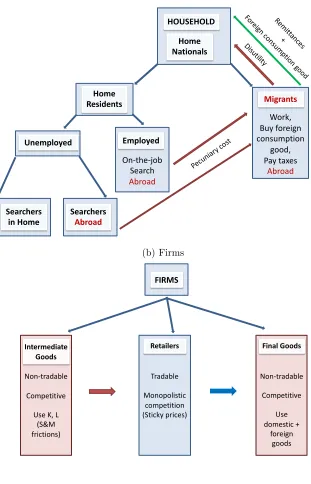
Our model introduces labour force mobility in a standard SOE model with search and match-ing frictions, sticky prices, and lack of monetary policy independence. The SOE is labeled Home. We consider in our calibration a scenario in which higher wages and more employment opportunities exist abroad than in Home. Hence, when we introduce endogenous migration decisions in the model, unemployed job seekers from Home will have an incentive to migrate abroad. Current workers may also have an incentive to migrate given higher wages and better fiscal conditions abroad. Apart from supplying labour, migrants pay taxes and consume part of their income abroad.

Home nationals are part of a representative household. In terms of their labour market status, household members can be employed or unemployed and participate in the domestic and the foreign labour markets.7 _{Searching for foreign jobs is subject to a pecuniary cost,}

whereas living abroad entails a utility cost (see, e.g., Hauser (2017)). Together with labour

7_{As discussed in Section 4.2 introducing endogenous labour force participation does not alter substantially}

supply decisions (hours), consumption and savings are defined at the household level.8 _On

the production side, following standard practice in the literature (see, e.g., Trigari (2006) and Erceg and Lind´e (2013)), we separate the decisions regarding factor demands from price setting to simplify the description of the model. In order to do this, we assume that there are three types of firms: (i) competitive firms that use labour and effective capital to produce a non-tradable intermediate good, (ii) monopolistic retailers that transform the intermediate good into a tradable good, and (iii) competitive final goods producers that use domestic and foreign produced retail goods to produce a final, non-tradable good. The latter is used for private and public consumption, as well as for investment. Price rigidities arise at the retail level, while labour market frictions occur in the sector producing intermediate goods. The government collects taxes and issues debt to finance public expenditure, lump-sum trans-fers, and the provision of unemployment benefits. For public spending we consider various roles, namely wasteful, productive and utility-enhancing spending. Implementation of debt consolidation occurs through labour income tax hikes or public spending cuts.

Finally, we note that the model features habit formation and investment adjustment costs, which are critical to generating smooth responses with reasonable degrees of nominal rigidities. In what follows below, the asterisk ⋆denotes foreign variables or parameters. We treat foreign variables as exogenous and therefore omit the time subscript. All quantities in the model are in aggregate terms, but we also present responses of per capita variables in the results that follow.

2.1

Home

2.1.1 Nationals, Residents and Migrants

We assume a continuum of identical households of mass one. In what follows we will refer to the representative household. The total number of Home nationals of the representative household is assumed to be constant and equal to ¯n. On the contrary, the number of Home

residents varies depending on changes in the stock of Home migrants abroad, with the latter

varying over time either due to new arrivals or due to returns back to Home. Denoting by

Nt the resident population and byne,t the stock of emigrant workers from Home, total Home nationals are given by

¯

n = Nt+ne,t. (1) 8_{See Andolfatto (1996) for an application of the big household assumption in a framework with}

At any point in time, Home residents are either employed nt or unemployed job seekers ut,

Nt = nt+ut. (2)

Among the unemployed job seekers ut, a share 1−st are searching in the domestic labour market, while the remaining st are looking for jobs abroad. Those who seek jobs abroad face an individual pecuniary cost ς(˜stu˜t), where ˜st and ˜ut are the average shares of st and ut per household and the function ς(˜stu˜t) is increasing in both arguments. This endogenous cost function (see Section 3 for the specific functional form) links positively the cost of search abroad with the number of unemployed who search for foreign jobs, helping to smooth out migration decisions in the model, putting a brake to the search abroad of the unemployed. In the domestic labour market, jobs are created through a matching function of the following form:

mt=µ1(υt)µ

2

((1−st)ut)1 −_µ2

, (3)

where mt denotes matches, υt denotes vacancies posted by firms,µ1 measures the efficiency

of the matching process andµ2 denotes the elasticity of the matching technology with respect

to vacancies.9 _{We define the probabilities of a job seeker to be hired ψ}

H,t and of a vacancy

to be filled ψF,t as follows:

ψH,t≡

mt (1−st)ut

and ψF,t ≡

mt

υt

.

Those currently employed in the domestic labour market nt can exert effort zt in searching for a job abroad where better labour market and fiscal conditions exist. The higher the search intensity, the higher the probability to be matched with a job abroad in the next period. We denote byϕ(zt) the productivity of on-the-job search effort measured in terms of the probability of finding a job abroad. Searching while employed is subject to a pecuniary cost φ(zt), measured in units of the final good. We assume that ϕ′(zt)>0 and φ′(zt)>0, with ϕ′(zt)

ϕ(zt) <

φ′_(z t)

φ(zt) such that on-the-job search effort is effectively costly (see, e.g., Krause and Lubik (2006) and T¨uzemen (2017)). The law of motion of employed workers in Home is given by

nt+1 = (1−σ−ψH⋆ϕ(zt))nt+ψH,t(1−st)ut, (4) 9_{A natural question is whether migration precedes search or search precedes migration. Given the}

where σ denotes the exogenous separation rate andψ⋆

Hϕ(zt) accounts for those workers that move abroad to join the measure of employed migrants.10

The law of motion for emigrant employmentne,t is then given by

ne,t+1 = (1−σ⋆)ne,t+ψH⋆ (stut+ϕ(zt)nt) . (5)

where for simplicity we assume that the job finding probability abroad for Home unemployed and employed is equal.

2.1.2 Households

The representative household consists of a continuum of infinitely lived agents. The house-hold derives utility from a consumption bundle Ct, composed of goods purchased by Home residents ct and by emigrants ce,t,

Ct = ct+ce,t, (6)

where ce,t is determined through (9) below.

To keep with the representative household framework, we assume that all agents pool consumption risk perfectly (for macro-labour models with migration and a representative agent, see, e.g., Kaplan and Schulhofer-Wohl (2017), Mandelman and Zlate (2012), Davis et al. (2014), and Binyamini and Razin (2008)). The household also suffers disutility from having members working abroad ne,t and from hours worked at home and abroad, htand he, respectively. The instantaneous utility function is given by

U(Ct, gtc, ht, ne,t) = Φ

1−η t

1−η −χ

h1+t ξnt+h1+e ξne,t

1 +ξ −Ω

(ne,t)1+µ

1 +µ , (7)

where Φt ≡ h

(1−α1)

Ct−ζC˜t−₁

α2

+α1(gtc,) α2i

1

α2

, gc

t, denotes utility-enhancing public expenditure,ηis the inverse of the intertemporal elasticity of substitution,ζ is the parameter determining external habits in aggregate consumption where the consumption reference is taken as given by the household, with ˜Ct = Ct−1 in equilibrium. The strictly positive parameters Ω, χ, µ and ξ are associated with the disutility from hours worked and from living abroad. The disutility from having family members abroad captures notions such as different culture, food, habits; distance from relatives and friends; less dense networks;

10_{Focusing on cross-country rather than within-country wage differentials, we abstract from on-the-job}

difficulties experienced with bureaucracy and integration, as well as families ties between the migrant and the non-migrant members of the household.11 _{Hours worked in Home h}

t are

determined through negotiation over the joint surplus of workers and firms (see below), while hours worked abroadheare taken as exogenous. The elasticity of substitution between private and public consumption is given by 1−_η

α2 . When this elasticity is greater than one, private

and public consumption are substitutes, while when it is below one, they are complements (see also Bermperoglou et al. (2017)). The Cobb-Douglas specification is obtained when the elasticity is equal to zero.

The budget constraint, in real aggregate terms, is given by

(1 +τc)ct+it+bg,t+etrf,t−₁b_f,t−₁ +ς(˜s_tu˜_t)s_tu_t+φ(z_t)n_t≤ (1−τn

t)wthtnt+

rk t −τ

k _rk t −δt

xtkt+rt−1bg,t−1+etbf,t+etΞt+ but+ Πpt +Tt, (8)

where ς(˜stu˜t)stut and φ(zt)nt are the total costs of search for jobs abroad for the unem-ployed and the emunem-ployed, respectively, wt is the hourly wage, rkt is the return on effective capital, b denotes unemployment benefits, et is the real exchange rate, and Πpt are profits from monopolistic retailers. The depreciation rate of capital is δt and the degree of capital utilization is xt. Lump-sum transfers and tax rates on private consumption, private capital, and labour income are given byTt,τc,τk,τtn, respectively. Government bonds are denoted by

bg,t, and pay the return rt, while bf,t denote liabilities with the rest of the world with return

rf,t.12 Migrants’ labour income is spent on purchases of goods abroad ce,t and remittances sent to Home, denoted by etΞt (in units of the Home final good),

Ξt+ (1 +τc⋆)ce,t = (1−τn⋆)w⋆hene,t. (9)

Following Mandelman and Zlate (2012), we assume a remittances rule of the following form:

Ξt=̺

(1−τn⋆_)w⋆ (1−τn

t )wt ρΞ

. (10)

The rationale behind (10) is that remittances represent an altruistic compensation mech-anism between migrant and domestic workers. Note that we do not include cross-country

11_{Including the utility cost of migration, in addition to the pecuniary costs of job search abroad, is useful in}

smoothing out migration decisions when we study the case of labour income tax hikes, which is the instrument that leads to the strongest increase in migration outflows. Without this utility cost, pecuniary costs would have to be unrealistically high in the simulations we perform in Section 4.

12

differentials in unemployment benefits as we do not intend to study those as drivers of the migration decisions of the household. In other words, assuming ρΞ > 0, a relative

improve-ment in the net wage premium abroad leads to an increase in remittances. Purchases of goods abroad ce,t is therefore modelled as the residual of the budget constraint of migrants once remittances are chosen (see also Mandelman and Zlate (2012)).13 _{As argued in the}

In-troduction (see footnote 4), evidence from World Bank data and from recent surveys suggests that the role of remittances has been very small in the recent emigration wave from Greece. This is captured in our calibration (see below).

The household owns the capital stock, which evolves according to

kt+1 =ǫi,t "

1− ω

2

it

it−1

−1

2#

it+ (1−δt)kt, (11)

where it is private investment, ǫi,t denotes an investment efficiency shock, which will be present in our simulations later on (see Section 4), and ω dictates the size of investment adjustment costs. Following Neiss and Pappa (2005), the depreciation rate δt depends on the degree xt, of capital utilization according to

δt= ¯δxιt, (12)

where ¯δ and ι are positive constants.

Given that he is exogenous, ce,t is determined through (9) and ht is determined through negotiation over the joint surplus of workers and firms (see below), the problem of the house-hold is to choose ct, kt+1, it, xt, bg,t, bf,t, nt+1, ne,t+1, st, zt to maximize expected lifetime utility subject to the budget constraint, the laws of motion of resident and migrant employ-ment, taking the probability of finding a job in Home and abroad as given, the law of motion of capital, the definition of capital depreciation, and the composition of the population. We report the full set of first order conditions in the Online Appendix and focus here on those that determine job seeking and migration.14 _{Denoting by λ}

c,t, λn,t and λe,t the Lagrange multipliers on the budget constraint and on the laws of motion of domestic and migrant employment, (4) and (5), the first order conditions with respect to nt+1, ne,t+1, st and zt are given by

13

We abstract from endogenizing the allocation of immigrant income between remittances and consumption of the foreign good, which would require to either assume that the household in Home makes this decision or to model migrants as separate optimizing agents. Given that remittances have increased much less than recent migration outflows from Europe’s periphery, as emphasized in the Introduction, endogenizing such choice is outside the scope of our paper.

λn,t = β "

λc,t+1((1−τtn)wt+1ht+1−b−φ(zt+1))−χ

h1+t+1ξ

1 +ξ

#

+β[λn,t+1(1−σ−ψH,t+1−ψH⋆ϕ(zt+1)) +λe,t+1ψH⋆ϕ(zt+1)], (13)

λe,t = β

λc,t+1((1−τn⋆)et+1w⋆he−b +ς(˜st+1u˜t+1))−χ

h1+ξ e

1 +ξ −Ω (ne,t+1)

µ

+β[λe,t+1(1−σ⋆−ψ⋆H)] , (14)

ψ⋆Hλe,t−λc,tς(˜stu˜t) = λn,tψH,t, (15)

λc,t

φ′ (zt)

ϕ′ (zt)

= ψ⋆

H(λe,t−λn,t) . (16)

Equations (13) and (14) determine the evolution of the value of being employed in Home and abroad, respectively. In both cases, the value for the household of a newly established match equates to the net direct utility gain, which is equal to the utility value of the net wage, where the latter is adjusted for the costs of searching abroad, minus the disutility from supplying hours and, for the case of equation (14), from having members abroad, plus the continuation value of the match.15 _{The latter is the expected value of continuing with}

the job without experiencing an exogenous separation, net of the value foregone because workers are not simultaneously job seeking, which is captured in equations (13) and (14) by

ψH,t+1 and ψ⋆H respectively. Equation (13) also accounts for the fact that with probability

ψ⋆

Hϕ(zt+1) a current worker will quit to take up a job abroad.16 Equation (15) shows that,

at the margin, the value of job seeking at home and abroad, with the latter including again the utility-adjusted cost of moving abroad, must be equalized. In other words, household members will not search for a job in Home when the value of searching abroad is higher, and vice versa. Finally, condition (16) states that, in equilibrium, the marginal costs of on-the-job search intensity, in units of consumption, must be equal to the excess value of working abroad relative to working in Home, subject to the probability of finding a job abroad. The higher this differential, the higher is the optimal level of on-the-job search.17

15_{Note that a new match becomes productive next period.}

16_{The Online Appendix includes the full derivation of equations (13) and (14). It is shown that the value}

of being employed in Home or abroad includes the full foregone value of being unemployed, which in turn consists of the value of the unemployment benefit and the value of being matched to a job.

17_{In the scenarios we analyze below, we only consider cases whereλ}

2.1.3 Intermediate goods firms

Intermediate goods are produced with a Cobb-Douglas technology,

yt = At(ntht)1 −α

(xtkt)α(gty,) ν

, (17)

where kt and nt are capital and labour inputs, xt is the degree of capital utilization, At is an exogenous stationary TFP process and gc

t, denotes the productive component of public expenditure. The parameter ν regulates how the public input affects private production: when ν is zero, government spending is unproductive.18

Since current hires give future value to intermediate firms, the optimization problem is dynamic, with firms maximizing the discounted value of future profits. The number of workers currently employed nt is taken as given and the employment decision concerns the number of vacancies υt posted in the current period, so as to employ the desired number of workers nt+1 in the next period. For firms, the law of motion of employment is given by

nt+1 = (1−σ−ψH⋆ ϕ(zt))nt+ψF,tυt,

which is equivalent to (4). Firms also decide the amount of effective capital xtktto be rented from the household at raterk

t. The problem of an intermediate firm withntworkers currently employed can be written as

Q(nt) = max xtkt,υt

px,tyt−wthtnt−rktxtkt−κυt+ Etβt+1Q(nt+1) ,

wherepx,t is the relative price of intermediate goods with the final good being the numeraire,

κ is the cost of posting a new vacancy, and βt+1 = βλct+1/λct is the household’s subjective discount factor. The maximization takes place subject to the law of motion of employment, where the firm takes the probability of the vacancy being filled as given. The first order conditions with respect to effective capital and vacancies are

rk

t = α

px,tyt

xtkt

, (18)

and

κ ψF,t

= Etβt+1

(1−α)px,t+1yt+1

nt+1

−wt+1ht+1+ (1−σ−ψ⋆Hϕ(zt+1))

κ ψF,t+1

. (19)

18_{Note that without the assumption of variable capital utilization all factors of production would be}

According to (18) and (19), the value of the marginal product of capital equals the real rental rate and the marginal cost of hiring an additional worker is set equal to the expected marginal benefit. The latter includes the marginal productivity of labour minus the wage plus the continuation value, knowing that with probabilityσthe match can be destroyed and that a termination can also occur due to cross-border job matches captured by ψ⋆

Hϕ(zt+1).

2.1.4 Wage bargaining

Wages are determined by splitting the surplus of a match between the worker and the firm according to their relative bargaining powers. Denoting by ϑ ∈ (0,1) the firms’ bargaining power, the splitting rule is given by (1−ϑ) (1−τn

t )StF = ϑStH , where StH denotes the worker’s surplus from a match in Home and SF

t denotes the surplus of the firm. The surplus for workers consists of the asset value of employment net of the outside option given by the value of being unemployed. As shown in the Online Appendix, the worker’s surplus from a match in Home can be written as

SH

t = (1−τtn)wtht−b−

χ λc,t

h1+t ξ

1 +ξ −φ(zt) +ϕ(zt)ς(˜stu˜t)

+ (1−σ−ψH,t−ϕ(zt) (ψH⋆ −ψH,t)) Etβt+1StH+1.

The introduction of on-the-job search affects the household’s decisions regarding job seeking and regarding also the allocation of job seekers’ search between Home and abroad through the impact on the asset value of being employed in Home. This asset value is negatively affected by the pecuniary costs of on-the-job search φ(zt) and the higher probability of leaving the job in the future due to successful on-the-job search effort, as given by the term ϕ(zt), and positively affected by the fact that, by being employed in Home, the worker avoids incurring search cost looking for a job abroad when unemployed ς(˜stu˜t).

Using the equation above together with the equivalent expression for the value of an additional employee abroad SF

h,t (see the Online Appendix), the definition of hiring rates, and the first order condition with respect to st, we obtain

ψH,tEt βt+1StH+1

= ψ⋆

HEt βt+1Sh,tF +1

−ς(˜stu˜t) .

which, in turn, will depend on the respective wage and separation rate. In turn, the firm’s surplus is given by

SF

t = (1−α)

px,tyt

nt

−wtht+ (1−σ−ψ⋆Hϕ(zt))

κ ψF,t

.

Using the above expressions, the negotiated real wage income wtht, determined by the split-ting rule of the Nash bargaining, is given by

wtht = (1−ϑ)

(1−α)px,tyt

nt

+ (1−ϕ(zt))

ψH,t

ψF,t

κ

+ ϑ

(1−τn t)

(

b + χ

λc,t

h1+t ξ

1 +ξ +φ(zt)−ϕ(zt)ς(˜stu˜t)

)

. (20)

The first term, weighted by the workers’ bargaining power (1−ϑ) includes the value of the marginal product of labour and the continuation value of the match to the firm, corrected by the continuation value of the match to the household. The presence of on-the-job search abroad affects this term through the possibility that workers can resign from their contracts. This is captured by (1−ϕ(zt)), which reflects the fact that the higher is on-the-job search, the lower the average tenure of work contracts in Home, pushing down on wages. The second term refers to the workers’ surplus and consists of the immediate outside option of being unemployed, corrected for the disutility from hours. This term is also affected by the pecuniary cost of on-the-job search φ(zt). Since, when employed, a worker incurs a cost from on-the-job search, the outside option must include the savings from not incurring this cost. Finally, the last term ϕ(zt)ς(˜stu˜t) appears because, in equilibrium, the worker surplus in Home and abroad must be equal taking into consideration the migration costs. The worker’s surplus from a match in Home includes an extra term to account for the fact that, by being employed in Home, the worker avoids incurring search cost looking for a job abroad when unemployed ς(˜stu˜t). The determination of hours in equilibrium through negotiation over the joint surplus of workers and firms is presented in the Online Appendix.

2.1.5 Retailers

coincides with the real marginal cost faced by the retailers. Letyi,t be the quantity of output produced by retailer i. These goods are aggregated into a tradable good, which is given by

yr,t =

Z 1

0

(yi,t)

ǫ−1

ǫ di

ǫ−ǫ1

.

where ǫ > 1 is the constant elasticity of demand for each variety of retail goods. The aggregate tradable good is sold at the nominal pricePr,t =

R

(Pi,r,t)ǫ −1

di

1

ǫ−1

, where Pi,r,t is the price of each variety i. The demand for each intermediate good depends on its relative price and on aggregate demand:

yi,t =

Pi,r,t

Pr,t −ǫ

yr,t.

We assume that in any given period each retailer can reset its price with a fixed probability 1 −λp. Firms that are able to reset their nominal price choose Pi,r,t∗ so as to maximize expected real profits given by

Πt (i) = Et ∞

X

s=0

(βλp)

sλc,t+s

λc,t

Pi,r,t

Pt+s

−px,t+s

yi,t+s

subject to the respective demand schedule, where Pt is the final good price. Since all firms are ex-ante identical, P∗

i,r,t = P ∗

r,t for all i. The resulting expression for the real reset price

p∗ r,t ≡P

∗ r/Pt is

p∗ r,t

pr,t

= ǫ

(ǫ−1)

Nt

Dt

(21)

with

Nt = px,tyr,t +λpEtβt+1(πr,t+1)ǫNt+1, (22)

Dt = pr,tyr,t +λpEtβt+1(πr,t+1)ǫ

−₁

Dt+1, (23)

wherepr,t ≡Pr,t/Ptandπr,t≡Pr,t/Pr,t−₁is the producer price inflation. Under the assumption of Calvo pricing, the price index in nominal terms is given by

(Pr,t)1 −ǫ

= λp(Pr,t−1)

1−ǫ

+ (1−λp) P ∗ r,t

1−_ǫ

The aggregate tradable good is sold domestically and abroad

yr,t = yl,t+ym⋆ , (25)

where yl,t is the quantity of tradable goods sold locally and ym⋆ the quantity sold abroad.

2.1.6 Final Goods Producer

Finally, perfectly competitive firms produce a non-tradable final good yf,t by aggregating domestic yl,t and foreign ym,t aggregate retail goods using a CES technology

yf,t = h

(̟)

1

γ (y_l,t) γ−1

γ + (1−̟)

1

γ (y_m,t) γ−1

γ

i_γ−γ1

. (26)

The home bias parameter ̟ denotes the fraction of the final good that is produced locally. The elasticity of substitution between home-produced and imported goods is given by γ. Final good producers maximize profitsyf,t−pr,tyl,t−etp⋆r,tym,t each period, wherepr,t and p⋆r,t denote the real price of aggregate retail goods produced in Home and abroad, respectively, and we have assumed the law of one price holds. Solving for the optimal demand functions gives

yl,t = ̟(pr,t) −γ

yf,t, (27)

and

ym,t = (1−̟) etp⋆r,t −γ

yf,t. (28)

We substitute out (27) and (28) into (26) to obtain

1 = ̟(pr,t)1 −γ

+ (1−̟) (etp⋆r)

1−γ

, (29)

where p⋆

2.1.7 Government

Government expenditure consists of unemployment benefits, public expendituregtand lump-sum transfers, while revenues come from conlump-sumption, capital income and labour income taxes. The primary deficit is, therefore, defined by

DFt= but+gt+Tt−τtnwthtnt−τk(rkt −δt)xtkt−τcct (30)

and the government budget constraint is given by

rt−₁bg,t−₁+DFt =bg,t. (31)

The composition of total government spending is given by

gt = gtw+gct +g y

t , (32)

where gw t , gtc, g

y

t denote the wasteful, utility-enhancing and productive components of public expenditure, respectively.

2.1.8 Resource constraint

The non-tradable final good is sold for private and public consumption, ct and gwt and for investmentit. However, costs related to vacancy posting and looking for a job abroad reduce the amount of resources available

yf,t = ct+it+gwt +κυt+φ(zt)nt+ς(˜stu˜t)stut. (33)

Aggregating the budget constraint of households using the market clearing conditions, the budget constraint of the government, and aggregate profits, we obtain the law of motion for net foreign assets, which corresponds to the current account and is given by

et(rf,t−₁bf,t−₁ −bf,t) = nxt+etΞt, (34)

where nxt are net exports defined as

The equation for exogenous exports is given by

ym,t⋆ =

pr,t

et γx

y⋆

m, (36)

where γx is the price elasticity of exports and ym⋆ is the steady-state level of exports pinned down by the calibrated value of steady-state net foreign assets.

In turn, real GDP is defined as

gdpt = yf,t+nxt. (37)

Using (25) and (35), together with the equilibrium condition yf,t = pr,tyl,t +etp⋆rym,t, real GDP can be equivalently expressed as

gdpt =pr,tyr,t. (38)

2.1.9 Lack of monetary policy independence

Regarding exchange rate policy, since the model is designed for peripheral countries of the euro area, such as Greece, we solve it for a case without monetary policy independence. Specifically, we assume that the nominal exchange rate E is exogenously set and, at the same time, the domestic nominal interest rate on domestic government bondsRtbecomes an endogenous variable (see, e.g., Erceg and Lind´e (2012)). The real exchange rate et is given by

et =

E·P⋆

Pt

.

The nominal interest rateRtis then pinned down endogenously through the Fisher equation19

rt =

Rt Etπt₊₁

. (39)

where consumer price inflation πt is defined as

πt =

Pt

Pt−₁

. (40)

19_{As noted in Philippopoulos et al. (2017), in the case of flexible or managed floating exchange rates, E}

Finally, we introduce a risk premium charged to Home households depending on the size of the deviation from its steady-state value of the net foreign liabilities to real GDP ratio,

rf,t = r⋆exp

Γ

etbf,t+1

gdpt

− ebf

gdp

+ǫr,t

(41)

where Γ is the elasticity of the risk premium with respect to liabilities (see Schmitt-Groh´e and Uribe (2003)), bf and e refer to the steady-state values of bf,t and et, and ǫr,t is a risk premium shock.

3

Calibration Strategy

We solve the model by linearizing the equilibrium conditions around a non-stochastic zero-inflation steady state in which all prices are flexible, the price of the final good is normalized to unity, and the real exchange rate is also equal to unity. We calibrate the model at an annual frequency with Greece as our primary target economy. Table 1 shows the key parameters and steady-state values we target.

National accounts

Using annual data from the Eurostat from 2008 to 2015, we set the shares of private con-sumption, capital investment and imports in GDP equal to 62% , 18%, and 25%, respectively. We also set net foreign assets and public debt to 10% and 127% of GDP, respectively, while remittances over GDP in the steady state are fixed to 3%, in line with World Bank data.

Utility function

a version of the model without the intensive margin. Using the FOC of the household with respect to gc,t in the steady state, and simplifying further by using the FOC with respect to

ct, allows us to pin down the following parameter value

α1 = 1 + (1 +τc)

C(1−ζ)

gc

1−_α2!

−₁

= 0.2925.

Following the literature on Edgeworth complementarity between private and public consump-tion goods (see, e.g., Bouakez and Rebei (2007), F`eve et al. (2013)), we set α2 =−0.75<0

so that private consumption and gc,t are complements.20

Production process

The capital share takes the standard value of 1/3 and the steady-state price markup over marginal costs is set to 10%. The annual depreciation rate is calibrated to 8.8% in order to match the ratio of capital investment to GDP above. The model’s steady state is independent of the degree of price rigidities and the size of the investment adjustment costs. The latter are included to moderate the response of investment with respect to fiscal shocks. We set the degree of price stickiness λp equal to 0.25, which is a standard value on an annual basis, and the degree of investment adjustment costs ωequal to 4. Using the FOC of the firm with respect to gy,t in the steady state allows us to pin down the following parameter value:

ν = gy

y = 0.05.

Labour market

We start by normalizing total Home nationals ¯nto unity, of which 10% reside abroad.21 _The

unemployment rate is set equal to 12%, which matches well the figure in Greece during 2009-2010. For simplicity, we assume that the termination rates in the domestic and foreign labour markets are both equal to 7%, which is the value used in Pappa et al. (2015). We set the vacancy-filling and job-finding probabilities equal to 0.70 and 0.60 respectively, which pins down the efficiency of the matching technology µ1. We calibrate the job-finding probability

20_{Note that the productive and utility-enhancing public goods are provided for free. However, to find their}

optimal levels, we equate the marginal productivity of each of the public goods to its price, which is equal to that of the private consumption good (our numeraire).

21_{Data from the UN Population Division at the Department of Economic and Social Affairs shows that the}

abroad to be 60% higher than in Home, which allows us to match an unemployment rate abroad of 7%, consistent with that of Germany in the same period. Using the laws of motion of employment in Home and abroad, our calibration implies a steady-state share of unemployed looking for a job abroad of 6.5%, whereas just below 0.5% of current workers are matched to a job abroad. Our calibration also implies that, in the steady state, 34% of migration outflows (household members who are newly matched with a job abroad) are current workers in Home who obtained a job abroad through on-the-job search effort. This number will be the starting point in our simulations for Greece for the period 2009-2015 in Section 4, where we will show that the model matches an average share of 48% over the entire period, in line with the survey evidence in Labrianidis and Pratsinakis (2016) mentioned in the Introduction. Vacancy-posting costs κ represent 15% of the wage, or, in the aggregate, just under 1% of GDP. Finally, we enforce the Hosios condition by setting the elasticity of matches to vacancies equal to the bargaining power of firms, µ2 =ϑ= 0.38 (see below).

Search abroad and migration

For the cost of job search abroad for the unemployed and the employed,ς(˜stu˜t) andφ(zt) re-spectively, as well as the productivity of on-the-job search effortϕ(zt) we adopt the following functional forms:

ς(˜stu˜t) =ςs1(˜stu˜t) ςs2

, φ(zt) = φz1(zt)φz

2

, ϕ(zt) = ϕz1(zt)

ϕz2

.

The scale parameters for search costs ςs1 and φz1, as well as the weight on the utility cost of

migration Ω, are implicitly determined by the first-order conditions (13) - (16) in the steady state. While ensuring realistic positive values for these parameters, we choose the remaining parameters by calibrating the net replacement rate b/[(1−τn)w] = 0.41 in line with data from the OECD Benefits and Wages Statistics, the bargaining power of firms ϑ= 0.38 in line with Flinn (2006), and the wage premium abroad w⋆_{/w = 1.10. These values imply that,} per job match abroad, search costs represent 46% and 36% of the wage for the unemployed and the employed respectively. Put differently, total costs of job search abroad account for around 0.33% of GDP. Note that the choice of a not very high wage premium abroad is driven by trying not to assume extremely high migration costs. We then normalize search effort z

to 1 and use the parameter for the on-the-job search effort productivity ϕz1 to determine the

steady-state number of workers that are matched to a job abroad. The remaining parameters

the magnitude of migration outflows in response to shocks. We set φz2 and ςs2 such that the

migration outflows in our simulations for Greece in Section 4 match (i) the total magnitude of migration outflows (equal to half a million people) presented in Lazaretou (2016) and (ii) the survey evidence in Labrianidis and Pratsinakis (2016) on the share of emigrants that were previously employed in Greece (close to 50%). Specifically, we calibrate ϕz2 jointly with φz2

so that the total number of workers emigrating in our simulations matches the Greek data and, at the same time, on-the-job effort fluctuates to reasonable values along the simulation horizon.22 _{Finally, the elasticity of the utility cost of living abroad µ is normalized to 1.}

The higher the value of µ, the lower the magnitude of the migration outflows. However, in the absence of costs to the number of workers abroad, the ratio of pecuniary searching costs to GDP would have to be unrealistically high for the model to reproduce the magnitude of outflows from Greece in our estimations. As presented below, the disutility of living abroad is associated with realistic results in the model about return migration over time after negative business-cycle shocks or a spending-based consolidation.

Policy

The elasticity of the spread between domestic and foreign interest rates Γ is set equal to 0.001. For the steady-state output shares of the government spending components, we use

gw_{/GDP = 0.0533, g}c_{/GDP = 0.1048 andg}y_{/GDP = 0.0512, based on annual Greek data} from Eurostat. Specifically, for gw _{we use Government’s Final Consumption Expenditure,} taking out compensation of employees (which we do not model) and consumption expenditure in the health and education sectors; for gy _{we use Government’s Gross Capital Formation} and forgc _{we use Government’s Expenditure in Health and Education, taking out the amount} used in these sectors for Gross Capital Formation to avoid double counting with the previous item.

4

Simulations for the Fiscal Policy Mix in Greece

We start by examining the predictions of our model when looking at the actual tax-spending consolidation implemented in Greece, which stands out as an example of public debt crisis and implementation of fiscal austerity policies. In 2010 Greece began the implementation of such measures in order to receive conditional bailout packages from international institutions.

22

In the analysis that follows, we present the results of three versions of the model: (i) without migration, (ii) with migration of the unemployed, and (iii) with migration of both the unemployed and employed. To compare the dynamics across the different specifications, we eliminate potential steady-state differences by working with the full model specification (iii), setting all variables related to migration and on-the-job search abroad to their steady-state values when considering the model specifications (i) and (ii).

4.1

Baseline simulations

We obtain annual data on the various components of public expenditure components from Eurostat. All paths are inputted into the simulation as shares of 2009 GDP. We allow lump-sum transfers to adjust to satisfy the government budget. As mentioned in Section 3, our calibration targets the magnitude and composition of the recent migration outflows in Greece. Specifically, we aim to to match (i) a total outflow of half a million until 2015 and (ii) a share of around 50% of emigrants that had a job before departure (Labrianidis and Pratsinakis (2016)). We construct effective taxes following the methodology of Mendoza et al. (1994). Figure 4a shows the number of emigrants by previous employment status, as generated by our simulations, and calculates the total amount of emigrants that left Greece until 2015. According to the results displayed, our simulations do a fairly good job in matching both (i) and (ii) above. Specifically, the model generates total migration outflows of 531,000 persons. This number matches very accurately the figure obtained through the Hellenic Statistic Authority (ELSTAT) for emigrants aged 15-64 during the period 2010-2015, which is 533,188. The share of previously employed predicted by the model is 51%.

We start the economy at its steady state and then feed in the model the actual annual values of the four fiscal consolidation instruments considered in the previous section for the period 2009-2015 (see Figure 4b). Under the informational assumption of random walk, the labour force expects the current fiscal policy stance to remain the same in the next period, so any change is entirely unanticipated. Given the annual frequency adopted here and given also that many ex post unanticipated changes in the fiscal packages were implemented in Greece due to failure of previous plans and mid-course revisions, we believe the use of the random-walk assumption is well justified. We proxy the macroeconomic environment in which the fiscal consolidation package was implemented through a combination of a risk premium shock and a negative investment shock. We include a table presenting information about the shocks used in the simulation exercise as well as the results of the exercise without the investment and risk premium shocks in the Online Appendix.

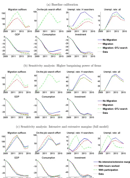
migration (solid lines), with migration of the unemployed (dashed lines) and with migration of both the unemployed and the employed (dash-dotted lines). As can be seen, the increase in migration outflows in the full model (dash-dotted lines) is of the magnitude observed in the data. The model also generates a significant increase in the intensity with which current workers look for employment abroad during the period 2010-2015. Consumption, investment, and GDP decline following closely the actual path of the data, which is depicted by the dot-ted lines for comparison. Specifically, the model without migration generates a fall in Greek output close to 20% after 2012, whereas the model with labour force mobility matches much more closely the actual fall in output of 25%. Regarding unemployment, the model also predicts a steady increase from 2010 onwards, even though its magnitude falls short of the data, according to which between 2010 and 2015 the unemployment rate in Greece almost doubled (from 13% to 25%). Note that for the unemployment rate we examine two mea-sures: “Unempl. rate: all” refers to all the Home residents who are unemployed, including those who look for jobs abroad while receiving the domestic unemployment benefit. As we can see, migration mitigates the increase of unemployment in the medium run. The second measure “Unempl. rate: H searchers” includes only the unemployed who look for domestic jobs, therefore excluding those who seek a job in the foreign labour market. As expected, this measure reveals a bigger difference in unemployment with and without labour mobility. We further investigate the unemployment response in the sensitivity analysis that follows.

4.2

Sensitivity analysis

In models with search and matching frictions the volatility of unemployment is somehow limited. However, as Panel 5b illustrates, if we raise the firms’ bargaining power to a higher value (equal to 0.7), we do get a much larger increase in unemployment (of around 60% higher than the steady-state level), as captured by the conventional measure .23 _{This happens}

because when the bargaining power of firms increases, the equilibrium wage level is closer to the outside option of households, given that the firm is able to extract a bigger share of the surplus of the match. When this is the case, the wage moves by less, given that the outside option of households is mostly determined by the unemployment benefit, which is fixed. This then makes firms decide to use the quantity margin (vacancies) by more since the wage is now less sensitive to shocks. As a result, there will be more unemployed. At the same time, wages moving by less means that on-the-job search effort for employment abroad increases by less. Finally, looking at the measure of the unemployment rate only for those searching domestically (“U rate: H searchers”) we see that the unemployment gains from emigration for the stayers are limited when both the unemployed and employed can migrate. Note that

with a longer time horizon we would likely observe in the medium run higher unemployment costs relative to the no-migration scenario, as discussed previously.

Finally, it is worth exploring in this exercise the role of the intensive versus the extensive margin. Recall that we have chosen to leave the latter out of our modeling specification so as not to blur the effects of migration on unemployment with the effects of labour force participation. Moreover, Greece exhibits very low probabilities of changing labour market status from inactivity to employment and vice versa (see Figure 5 in Garda (2016)). Panel 5c reports our simulations for the full model (with migration of both the unemployed and the employed) for three specifications: the dashed lines now repeat the results shown in Panel 5a for the model with hours, the solid lines show the results when we remove hours from the model, and the dashed-dotted lines report the responses when we include endogenous labour force participation, instead of hours, in the model.24 _{As can be seen, the main differences}

appear in the response of the unemployment rate. When we remove hours from the model, we tend to obtain a bigger increase in medium-run unemployment but a smaller increase in migration outflows, while with endogenous labour force participation, the increase in the conventional measure of unemployment (“U rate: all”) occurs faster. At the same time, the unemployment rate for those searching domestically (“U rate: H searchers”) increases, rather than decreases, in the short run, driven by the increase in labour force participation due to the negative income effect of the risk-premium shock.25

5

Migration Over the Business Cycle

In this section we examine the responses of the main macroeconomic and labour market variables to standard business cycle shocks, namely a negative supply shock (to TFP) and a negative demand shock (to the risk premium), which we assume follow an auto-regressive form with one lag and coefficient ρ = 0.75. The goal is to examine the behaviour of

mi-24

We modify the utility function as follows

U(Ct, gtc, ht, ne,t) = Φ1−η 1−η −χ

h1+_t ξnt+h1+e ξne,t

1 +ξ −Ω

(ne,t)1+µ 1 +µ +X

l1−ϕl t 1−ϕl

, (42)

where X > 0 is the relative preference for leisure, which is pinned down in steady state by the first-order condition with respect to unemployment (see the Online Appendix), setting in steady statel= 1/3, andϕl is the inverse of the Frisch elasticity of labour supply, which takes the standard value 4 in our calibration.

25

gration variables and the impact of migration on economic aggregates in comparison to a counterfactual scenario of labour force immobility.

5.1

TFP shock

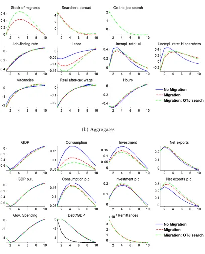
Figure 6 reports the responses of the model for a negative TFP shock. Panel 6a shows the migration and labour market variables, while Panel 6b refers to the main aggregates in the economy. The solid lines for the model without migration confirm that a negative TFP shock leads to a decrease in vacancies and the real wage, given the drop in the marginal product of labour. The job finding rate falls and pushes down on employment. As a result, the unemployment rate rises. Due to sticky prices, markups decrease and so the drop in profits becomes larger than the decrease in wages. Because the labour-increasing income effect of lower profits dominates the labour-reducing effect of lower wages, hours rise. We also observe a decrease in consumption, investment and GDP in the economy. Given the negative supply shock, prices go up. On the other hand, the decrease in demand leads to a decrease in imports and therefore a rise in net exports.

capita GDP actually falls by less, while the response of per capita investment hardly differs between the two models. The higher fall in consumption in the model with migration relative to the specification without migration is preserved in per capita terms, but is smaller in mag-nitude, as expected. On the other hand, the positive response of net exports is significantly reinforced in per capita terms. The latter outcome explains the fact that per capita GDP falls by less with migration relative to the benchmark model of immobility.

The dash-dotted lines present the impulse response functions when we introduce in the model on-the-job search abroad. After a negative TFP shock, workers increase substantially the intensity with which they look for jobs abroad, which reinforces the increase in the stock of migrants and the reduction employment relative to the previous two versions of the model. At the same time, the search abroad of unemployed job seekers is mitigated, since the exodus of workers due to successful matches abroad leads firms to cut vacancies by less, attenuating the decrease in the domestic job finding rate. Consequently, the positive impact of labour mobility on the short-run unemployment rate is mitigated. However, over time, these unemployment gains from migration are reversed due to the stronger contraction in employment. We also observe a decrease in the intensity of on-the-job search abroad below its steady-state level. In aggregate terms, internal demand and GDP fall by more than in the previous two versions of the model. Again, looking at per capita measures, we see that actually per capita GDP falls by less than in the previous two versions of the model due to the stronger increase in per capita net exports. The negative impact of labour mobility on consumption is preserved but weakened in per capita terms.

In sum, a negative TFP shock increases the search abroad of unemployed job seekers for many periods, which has a positive impact on short-run unemployment, but also reinforces the negative effects of the shock on consumption and leads to higher unemployment costs over time. Taking into account also the job search abroad of current workers reinforces the fall in consumption, mitigates the short-run unemployment gains from migration and reinforces unemployment costs over time.

5.2

Risk premium shock

lower wages and markups. All other responses are in line with the results presented in Section 5.1 for a negative TFP shock. Specifically, an increase in the risk premium induces a higher fraction of unemployed searching for foreign jobs in the short run, which has a positive impact on short-run unemployment, but also reinforces the negative effects on consumption. Taking into account also the job search abroad of current workers reinforces the fall in consumption, mitigates the short-run unemployment gains from migration and reinforces unemployment costs over time.

Note that the main variables react similarly to the TFP and risk premium shocks, in-cluding all the labour market variables and emigration in particular. This suggests that the primitive cause of the recession does not seem to be crucial for these results. However, the two shocks differ with respect to the response of inflation, which increases after a TFP shock, while it decreases after a risk premium shock.

6

Migration and Fiscal Consolidation

In this section, we compare the effects of tax hikes versus spending cuts by considering one fiscal consolidation instrument at a time.

6.1

Adding fiscal consolidation in the model

Let us assume that government has two potential fiscal instruments, labour income tax rates

τn

t and public expenditure g f

t where f = w, c, y for the different components of spending (i.e. wasteful, consumption, productive). The other tax rates, τk _{and τ}c_{, are treated as} parameters. We will consider each instrument separately, assuming that if one is active, the other remains fixed at its steady state value. For Ψ ∈ {τn_{, g}f_{}, following Erceg and} Lind´e (2013) and Pappa et al. (2015), we assume fiscal rules according to which the fiscal instruments depend on the discrepancy between the debt-to-GDP ratio ˜bg,t ≡ _gdpbg,t

t and an exogenous target bT

g,t, and also on the discrepancy between their changes, denoted by ∆. Specifically, we assume

Ψt = Ψ(1 −βΨ0)

ΨβΨ0

t−1





˜_bg,t

bT g,t

!βΨ1

∆˜bg,t+1

∆bT g,t+1

!βΨ2

 (1−_βΨ0)

, (43)

where βΨ1, βΨ2 > 0 for Ψ = τn, and βΨ1, βΨ2 < 0 for gf. The target debt-to-GDP ratio is

given by the AR(2) process

logbT

g,t−logbTg,t−₁ =ρ1(logb T

g,t−₁−logb T

g,t−₂) +ρ2(log¯b−logb T

g,t−₁)−ε b

where ¯b is the steady-state level of the debt-to-GDP ratio, εb

t is a white noise process repre-senting a fiscal consolidation shock, 0 ≤ ρ1 < 1 and ρ2 > 0. By introducing strong inertia

through the AR(2) process, we therefore consider a gradual (effectively permanent) reduction in the target for the debt-to-GDP ratio (see also Erceg and Lind´e (2013), Pappa et al. (2015), Bandeira et al. (2018)).26

Below we consider a shock that drives the debt-to-GDP target bT

g,t, determined by (44), 5% below its steady state. We simulate the responses to this shock with labour income taxes or government spending adjusting through (43) so that the actual debt-to-GDP ratio ˜bg,t meets the new lower target after 10 years in the benchmark specification without migration. In this way, we can ensure comparability for the tax-spending instruments, given the same size and timing of fiscal consolidation in the baseline economy without migration. When we introduce subsequently migration decisions for the unemployed and the employed, we maintain the same fiscal rule parameters βΨ0, βΨ1, βΨ2 (see Table 2). We calibrate the debt

target rule (44) setting ρ1 = 0.6 and ρ2 = 0.000001 so that about half of the convergence

to the new long-run debt target is achieved after five years, and that the debt target is fully implemented after 10 years (see Erceg and Lind´e (2013)).27 _{For the fiscal rule (43), we}

calibrate the set of three parameters for each fiscal instrument in such a way that the actual debt-to-GDP ratio ˜bg,t meets the new, lower target at the same time across the different instruments and at 10 years after the decision to consolidate is taken.

6.2

Labour tax hikes

We begin with the case of tax-based consolidation, depicted in Figure 8 where Panel 8a shows the migration and labour market variables, while Panel 8b refers to the main aggregates in the economy. Starting with the model without migration (see solid lines), we can see that consumption and investment fall, given the drop in after-tax income. The drop in demand leads to a fall in vacancies, the job finding probability, and employment, while unemployment rises. The labour tax hike also decreases hours by affecting negatively the incentives to work. The fall in internal demand leads to a fall in the demand for imports, reflected in the increase of net exports, but the contraction in internal demand is stronger and so real GDP falls.

When we introduce job search abroad for the unemployed (see dashed lines), the sig-nificant fall in the job-finding probability induces the household to increase the share of foreign-job seekers, leading to a higher stock of migrants. Vacancies and employment fall substantially more, given the stronger contraction in demand. Due to the fact that more

26_{Note that studying the possibility of sovereign default is beyond the scope of our paper.}

27_{In line with Erceg and Lind´e (2013), the debt target is eventually assumed to converge back to the steady}