This is a repository copy of
Distributed Secondary Frequency Control Design for
Microgrids: Trading Off L2-Gain Performance and Communication Efforts under
Time-Varying Delays
.
White Rose Research Online URL for this paper:
http://eprints.whiterose.ac.uk/128268/
Version: Accepted Version
Proceedings Paper:
Alghamdi, S, Schiffer, JF orcid.org/0000-0001-5639-4326 and Fridman, E (2018)
Distributed Secondary Frequency Control Design for Microgrids: Trading Off L2-Gain
Performance and Communication Efforts under Time-Varying Delays. In: 2018 European
Control Conference (ECC). 2018 European Control Conference, 12-15 Jun 2018,
Limassol, Cyprus. IEEE . ISBN 978-3-9524-2698-2
10.23919/ECC.2018.8550506
© EUCA 2018. Personal use of this material is permitted. Permission from IEEE must be
obtained for all other uses, in any current or future media, including reprinting/republishing
this material for advertising or promotional purposes, creating new collective works, for
resale or redistribution to servers or lists, or reuse of any copyrighted component of this
work in other works.
[email protected] https://eprints.whiterose.ac.uk/
Reuse
Items deposited in White Rose Research Online are protected by copyright, with all rights reserved unless indicated otherwise. They may be downloaded and/or printed for private study, or other acts as permitted by national copyright laws. The publisher or other rights holders may allow further reproduction and re-use of the full text version. This is indicated by the licence information on the White Rose Research Online record for the item.
Takedown
If you consider content in White Rose Research Online to be in breach of UK law, please notify us by
Distributed Secondary Frequency Control Design for Microgrids: Trading
Off
L
2
-Gain Performance and Communication Efforts under Time-Varying
Delays
Sultan Alghamdi, Johannes Schiffer and Emilia Fridman
Abstract— Consensus algorithms are promising control schemes for secondary control tasks in microgrids. Since con-sensus algorithms are distributed protocols, communication efforts and time delays are significant factors for the control design and performance. Moreover, both the electrical and the communication layer in a microgrid are continuously exposed to exogenous disturbances. Motivated by this, we derive a synthesis for a consensus-based secondary frequency controller that guarantees robustness with respect to time-varying delays and in addition provides the option to trade offL2disturbance
attenuation against the number of required communication links. The efficacy of the proposed approach is illustrated via simulations based on the CIGRE benchmark medium voltage distribution network.
I. INTRODUCTION
A. Motivation and Related Work
The rapid deployment of distributed renewable energy sources poses tremendous challenges for power system con-trol and operation [1]. In particular, the replacement of a few bulk conventional power plants with a large number of small-scale renewable generators significantly increases the complexity of coordinating demand and generation in real-time. Clearly, in such a setting centralized solutions are inappropriate and instead distributed architectures need to be developed. In that spirit, the microgrid (MG) concept has been identified as a core element of future power systems [1], [2]. A MG is a small-scale power system, which is composed of a combination of distributed generation units, energy storage devices and loads at the distribution level, with the ability to operate either in grid-connected mode or islanded mode [1], [3]. Thus, future power systems could be operated as a cell-structure of interconnected MGs.
For this type of networks many new control challenges arise [4]. Amongst these, frequency regulation is a fun-damental operational objective [2], [4]. As in bulk power systems, in MGs this objective is typically realized via a hierarchical control layer consisting of primary, secondary and tertiary control [4], [5]. While the primary controllers are usually implemented in a completely decentralized manner [4], the secondary control layer requires (distributed) integral
S. Alghamdi and J. Schiffer are with School of Electronic & Elec-trical Engineering, University of Leeds, United Kingdom, LS2 9JT
{elsalg,j.schiffer}@leeds.ac.uk
E. Fridman is with Tel-Aviv University, Israel
J. Schiffer acknowledges funding from the European Union’s Horizon 2020 research and innovation programme under the Marie Skłodowska-Curie grant agreement No. 734832 and E. Fridman acknowledges funding from the Israel Science Foundation (grant no. 1128/14).
action, in order to restore the frequency to its nominal value following a change in the systems’ power balance [4], [5].
In recent years, distributed consensus-based algorithms have gained increasing popularity for secondary frequency control in MGs [6]–[10]. Consensus protocols are distributed protocols and peer-to-peer communication between partici-pating units is essential for their implementation. Thus, the design of the communication network and the robustness of the closed-loop system with respect to communication uncer-tainties, such as time delays and exogenous disturbances, is of paramount importance [2]. Likewise, the electrical layer of the MG is continuously exposed to perturbations, e.g., in the power demand. Robustness of consensus-based secondary controllers with respect to delays has been investigated in [11]–[13], but the analysis is either limited to a linearized (small-signal) model or does not consider the electrical dy-namics and is partially restricted to constant delays. Bounded input-output performance of linearized models of secondary controlled MGs has been considered using the H2-norm in
[10] and theH∞-norm in [14]. A very similar setup for bulk
power systems with distributed frequency control is employed in [9], where in addition to minimizing the H2-norm also
sparsity of the communication network is promoted. Yet, the simultaneous consideration of these three objectives has not been reported in the literature.
B. Contributions
As a consequence of the above discussion and extending our previous work on delay-robust stability analysis [15], the main contribution of the present paper is a design procedure for consensus-based secondary frequency controllers in MGs, which jointly considers the objectives of delay robustness, bounded L2-gain performance for disturbance attenuation
(i.e., the maximum energy amplification ratio of the system) and sparsity of the communication network.
Inspired by related work on sparsity-promoting control for power systems and MGs [9], [16], [17], we use the (re)weighted ℓ1-norm as a proxy for the sparsity of the
communication network, see also [18]. Then we formulate the proposed robust and sparsity-promoting control synthesis as a convex optimization problem, which is derived for a nonlinear MG model via the Lyapunov-Krasovskii and the descriptor methods [19]. The employed cost function provides the option to trade offL2-gain performance against
the number of communication links.
|π
2|). Thus, if it is feasible, the desired performance
specifica-tions hold true in a wide range of operating condispecifica-tions. This is illustrated via numerical experiments using the CIGRE benchmark medium voltage (MV) distribution network [20].
Notation. We define the sets R≥0 := {x ∈ R|x ≥ 0}, R>0 := {x ∈ R|x > 0} and R<0 := {x ∈ R|x < 0}.
For a setV,|V|denotes its cardinality and[V]k denotes the
set of all subsets of V that contain k elements. Let x :=
col(xi)∈Rndenote a vector with entriesxifori= 1, . . . , n, 1n the vector with all entries equal to one, In the n×n
identity matrix, 0 a zero matrix of appropriate dimensions
and diag(ai), i = 1, . . . , n an n×n diagonal matrix with diagonal entries ai ∈ R. For A ∈ Rn×n, A > 0 (A < 0)
means that A is symmetric positive (negative) definite. The lower-diagonal elements of a symmetric matrix are denoted by ∗. We denote by W[−h,0], h∈R>0, the Banach space
of absolutely continuous functions φ : [−h,0]→ Rn, h ∈
R>0, with φ˙ ∈ L2(−h,0)n and with the norm kφkW = maxθ∈[a,b]|φ(θ)| +
R0
−hφ˙
2dθ0.5. Also,
∇f denotes the gradient of a functionf :Rn→R.
II. PRELIMINARIES A. L2-Gain of Dissipative Systems
We briefly recall some standard results on dissipative systems based on [21], [22]. Consider the state space system
˙
x=f(x, u), x∈Rn, u∈Rm,
y=h(x, u), y∈Rp. (II.1)
Definition 2.1: [21] The state space system (II.1) is dis-sipative with respect to the supply rate s : Rm×Rq → R
if there exists a functionS :Rn →R≥0, called the storage
function, such that for allx0∈Rn, allt1≥t0 and all input
functionsu,
S(x(t1))≤S(x(t0)) +
Z t1
t0
s(u(t), y(t))dt.
Definition 2.2: [21] The system (II.1) has a L2-gain less
than or equal toγif it is dissipative with respect to the supply rate s(u, y) =1
2(γ 2
kuk2
− kyk2).
Based on [22, Definition 6.2], we employ the following notion of asmall-signalL2-gain.
Definition 2.3: The system (II.1) has a small-signal L2
-gain less than or equal toγif it is dissipative with respect to the supply rates(u, y) = 12(γ2
kuk2
− kyk2) for allu ∈L2
withsup0≤t≤τkuk ≤rfor some positive real constantr.
B. Algebraic Graph Theory
An undirected weighted graph of order n is a triple
G= (V,E, z), with set of nodes V = {1, . . . , n}, set of undirected edges E ⊆[V]2,
E ={e1, . . . , em}, m=|E|and
weight function z : E → R≥0. By associating an arbitrary
ordering to the edges, the node-edge incidence matrix B ∈
R|V|×|E| of an undirected graph is defined element-wise as
bil= 1,if nodeiis the source of thel-th edgeel, bil=−1,
if i is the sink of el and bil = 0 otherwise. The Laplacian
matrix of an undirected weighted graph is given by [23], [24]
L=BZB⊤, Z=diag(zl), (II.2)
wherezl≥0is the weight of thel-th edge,l= 1, . . . , m. An
ordered sequence of nodes such that any pair of consecutive
nodes in the sequence is connected by an edge is called a path. A graphG is called connected if for all pairs {i, k} ∈ [V]2 there exists a path fromitok. The Laplacian matrix
L
of an undirected graph is positive semidefinite with a simple zero eigenvalue if and only if the graph is connected. The corresponding right eigenvector to this simple zero eigenvalue is1n, i.e.,L1n=0n [24]. We refer the reader to [23], [24]
for further information on graph theory.
III. MICROGRIDMODEL WITHDISTRIBUTED
SECONDARYFREQUENCYCONTROL ANDTIMEDELAY
A. Microgrid Model
We consider a Kron-reduced representation of a MG with mixed generation pool consisting of rotational and electronic-interfaced units [5], [25]. The set of nodes is denoted by
N ={1,· · · , n}, n≥1.Following standard practice [5], [6], [15], we assume that the line admittances are purely inductive and that the voltage amplitudesVi ∈ R>0 at all nodes are
constant. This assumption is admissible in MG analysis, since the inverter output impedance is typically highly inductive [6], [26]. Then, two nodesiandkare connected via a non-zero susceptance Bik ∈R<0. If there is no line between i
andk,thenBik= 0. We denote the set of neighboring nodes
of nodeibyNi ={k∈ N |Bik= 0}. We assume that for all
{i, k} ∈[N]2there exists an ordered sequence of nodes from itoksuch that any pair of consecutive nodes in the sequence is connected by a power line represented by an admittance, i.e., the electrical network is connected. We assign to each node a phase angle θi:R≥0→R and a frequency ωi = ˙θi
and defineθ=col(θi) andω =col(ωi). With the potential functionU :Rn→R,
U(θ) =− X
{i,k}∈[N]2
|Bik|ViVkcos(θik),
the active power flowsP :Rn→Rn can be written as P(θ) =∇U(θ).
Furthermore, we assume that all units are equipped with the standard frequency droop controller [4], [5], [25]. Then, the MG dynamics can be compactly written as [25], [26]
˙ θ=ω,
Mω˙ =−D(ω−1nωd)− ∇U(θ) +Pnet+u, (III.1)
where D = diag(Di) ∈ Rn
>0 is the matrix of (inverse)
droop coefficients, ωd ∈ R
>0 is the reference frequency
andu:R≥0→Rn is the secondary frequency control input.
Moreover, the matrix of (virtual) inertia coefficients is given by M=diag(Mi)∈Rn
>0, where for any inverter-interfaced
unit Mi=τpiDi withτpi∈R>0 being the time constant of
the power measurement filter. In addition, Pnet is given by
Pnet=
col(Pd
i −GiiVi2), where Pid ∈R denotes the active
power set point andGiiVi2, Gii∈R≥0, represents the active
power demand at thei-th node. See [3] for further details on the modeling of the system components.
B. Secondary Frequency Control: Objectives and Distributed Control Scheme
Suppose that the solutions of the system (III.1) evolve along a motion with constant frequencyωs=1
Then, summing over all frequency dynamics yields
1⊤
nMω˙s= 0 ⇒ ω∗=ωd+
1⊤
nPnet+1⊤nu∗
1⊤
nD1n
, (III.2)
where we have used the fact that1⊤
n∇U(θ) = 0.A standard
requirement in power system operation is thatω∗=ωd,i.e.,
the network synchronizes to the nominal frequency [4], [5]. However, in practice, the load demandsGiiVi2 contained in Pnetare unknown and thus, typically,1⊤
nPnet6= 0.Therefore,
the control inputsu∗have the task to compensate this power imbalance such that indeedω∗=ωd,see (III.2). This task is
termed secondary frequency control [4], [5].
Let A ∈ Rn>×0n be a diagonal positive definite weighting
matrix, K ∈ Rn>×0n be a diagonal feedback gain matrix
and L ∈ Rn×n be the Laplacian matrix of an undirected and connected graph with incidence matrix B and diagonal matrix of nonnegative edge weights Z, see (II.2). Consider the distributed secondary frequency control [6], [15]
u=−p, p˙=K(ω−1nωd)−KALAp(t−τ), (III.3)
where τ : R≥0 → [0, h], h ∈ R≥0, denotes a fast-varying
delay [19], [27]. Physically, this delay represents communi-cation delays between different nodes in the network. As a consequence of digital control [19] and the communication network conditions [28] this delay may be time-varying.
It has been shown in [29], [30], that the control (III.3) restores the frequency to its nominal value, while ensuring economic optimality in a synchronized state, i.e.,
Aiiusi =Akkusk ∀i∈ N, ∀k∈ N.
Thus, usually the matrix A is fixed by economic considera-tions. Hence, given (III.3), the distributed secondary control design problem consists in suitably determining the matrices
K andL. This problem is addressed in the present paper.
C. Closed-Loop System
Combining (III.1) with (III.3) yields
˙ θ=ω,
Mω˙ =−D(ω−1nωd) +Pnet−p− ∇U(θ), ˙
p=K(ω−1nωd)−KALAp(t−τ).
(III.4)
For the subsequent controller synthesis, the following notion is useful, see also [15], [26].
Definition 3.1: The system (III.4) admits a synchronized motion if it has a solution for all t≥0 of the form
θs(t) =θ0s+ωst, ωs=ω∗1n, ps∈Rn,
whereω∗∈Randθs
0∈Rn are such that |θs
0,i−θ0s,k|< π
2 ∀i∈ N, ∀k∈ Ni.
It has been shown in [29], [30] that the system (III.4) possesses at most one synchronized motion and that this motion satisfies
us=
−ps, ps=λA−11
n, λ=
1⊤
nPnet
1⊤
nA−11n .
IV. CONTROLLERSYNTHESIS A. Coordinate Transformation and Error System
Following the approach in [15], we perform both a co-ordinate transformation and reduction that are instrumental
to our synthesis. Let K = κK, where K ∈ Rn×n is a diagonal matrix with positive diagonal entries and κ > 0
is a parameter. Note that the fact thatL1n=0n yields to an
invariant subsystem in thep-variables. Consider the change of coordinates
¯ p ζ
=W⊤(κK)−1
2p, W =
h W √1
µK−
1 2A−11
n i
, (IV.1)
whereW ∈Rn×(n−1)is chosen such thatW⊤K−1 2A−11
n=
0n−1 and µ =kK−12A−11
nk22. Hence, the column vectors
of W form an orthonormal basis that is orthogonal to
K−12A−11
n. Thus, the transformation matrix W ∈ Rn×n
is orthogonal. By using (IV.1) and following the procedure in [15, Section 3.2], we can represent the closed-loop system (III.4) in new reduced order coordinates by
˙ θ=ω,
Mω˙=−D(ω−1nωd) +Pnet− ∇U(θ)−(κK)12Wp¯
−κµA−11n(1⊤
nA−1(θ−θ0−1nωdt+κ−1K−1p0),
˙¯
p=κ12W⊤K 1 2(ω−1
nωd)−κW⊤K
1 2ALAK
1
2Wp¯(t−τ),
(IV.2) where we have expressed the variableζin (IV.1) in terms of
θ, ωd,θ
0andp0, see [15] for details. We make the following
standard assumption [15], [26].
Assumption 4.1: The system (IV.2) possesses a synchro-nized motion.
With Assumption 4.1, we define the error states
˜
ω=ω−ωs, θ˜=θ0−θ0s+
Z t
0
˜ ω(τ)dτ,
˜
p= ¯p−p¯s, x=col(˜θ,ω,˜ p˜).
Then, the error system corresponding to (IV.2) is given by
˙˜ θ= ˜ω,
Mω˙˜=−Dω˜− ∇U(˜θ+θs) +∇U(θs)−(κK)1 2Wp˜
−1µκA−11
n1⊤nA−1θ˜+dω, ˙˜
p=κ12W⊤K 1
2ω˜−κW⊤K 1 2ALAK
1
2Wp˜(t−τ) +d
p,
y=colW
1 2
1 ω, W˜
1 2
2 p˜
, d=col(dω, dp),
(IV.3) where we have added the disturbance inputsdω anddp, as
well as—inspired by [9]—defined the performance outputy
with weighting matrices
W1=M >0, W2=W⊤K
1 2W¯
2K
1 2W,
¯
W2=In− 1
1⊤
nA−11n A−121
n1⊤nA−
1 2.
(IV.4)
Note thatW2quantifies the deviation of the controller states
from their average (scaled by κ−1A1
2) and W
1 accounts
for the system’s kinetic energy. Moreover, with Assump-tion 4.1, the system (IV.3) has an equilibrium point xs =
col(˜θs,ω˜s,p˜s)at the origin.
B. Problem Statement
desired properties. Compared to existing work, e.g., [6], [8]– [10], our proposed design takes robustness with respect to time-varying delays and external perturbations into account, while minimizing the required communication efforts, i.e., the number of network links.
With regard to the number of communication links, an obvious approach is to, in addition to the L2-gain,
min-imize the 0-norm of the vector Z1m, i.e., kZ1mk0 =
{number ofzi|zi 6= 0} (recall from (II.2) that Z ≥ 0 is a
diagonal matrix). Yet, the difficulty in using this approach is that the problem is convex. To overcome the non-convexity, the ℓ1-norm kZ1mk1 = Pmi=1|zi| is often used
as a convex relaxation of the 0-norm [9], [17], [18]. To improve this relaxation, the reweightedℓ1-normkWZZ1mk1
can be used [18], where the diagonal entries of the diagonal matrixWZ are chosen aswZ,i= (zi+υ)−1, i= 1, . . . , m,
withυbeing a small positive number. This, however, implies that an iteration scheme is needed, since the assigned values of the weighting matrix WZ depend on the solution of the
optimization problem. Alternatively, in the MG case power system engineering insights could be used to determine the weighting matrix WZ, see also [17]. The above discussion leads to the following problem statement.
Problem 4.2: Consider the system (IV.3) with Assump-tion 4.1. Determine κ and Z, such that given h ∈ R≥0
with τ ≤ h, xs = 0
3n−1 is a uniformly asymptotically
stable equilibrium point of the system (IV.3), the system (IV.3) is dissipative with respect to the supply rates(d, y) =
1
2(γ2kdk22 − kyk22), where d and y are given in (IV.3),
and the number of communication links is minimized, i.e.,
minZ≥0trace(Z).
C. Main Result
In this section, we provide a solution to Problem 4.2. Recall the definition ofLin (II.2). To present our main result, it is convenient to introduce the scaled matrix of edge weights and the corresponding scaled Laplacian matrix, i.e.,
¯
Z =κZ, L¯=K12ABZ B¯ ⊤AK 1
2. (IV.5)
Proposition 4.3: Consider the system (IV.3) with Assump-tion 4.1. Recall the weighting matricesW1 andW2given in
(IV.4). Fix h≥ 0, K >0 and ε > 0 as well as weighting parameters α >0, β > 0 and a diagonal weighting matrix
WZ > 0. Suppose that there exist parameters κ >¯ 0 and matrices Z ≥¯ 0, R > 0, S > 0 and S12, such that the
following optimization problem is feasible:
min
¯
γ,κ,¯Z¯ α¯γ−βκ¯+trace WZ
¯
Z
subject to
Q=
Q11 0 Q13 0 0 12In 0
∗ Q22 −14In−1S12 Q25 0 12In−1 ∗ ∗ Q33 0 Q35 0 14εIn−1
∗ ∗ ∗ Q44 Q45 0 0
∗ ∗ ∗ ∗ Q55 0 0
∗ ∗ ∗ ∗ ∗ Q66 0
∗ ∗ ∗ ∗ ∗ ∗ Q77
<0,
R S12
∗ R
≥0,
(IV.6)
where
Q11=−D+0.5W1, Q13= 0.25ε¯κK
1 2W, Q
22=S−R+0.5W2, Q25=R−S12−0.5W⊤L¯W, Q33=−0.5εIn−1+h2R,
Q35=−0.25εW⊤L¯W , Q44=−S−R, Q45=R−S12⊤, Q55=−2R+S12+S⊤12, Q66=−0.5¯γIn, Q77=−0.5¯γIn−1.
Choose the controller parameters as
κ= ¯κ2,
L= 1 κBZB¯
⊤. (IV.7)
Then, for all τ(t)∈[0, h], the origin is a locally uniformly asymptotically stable equilibrium point of the system (IV.3) and the system has a small-signalL2-gain less than or equal
to γ = √γ¯ with respect to the supply rate s(d, y) =
1 2 γ
2 kdk2
2− kyk22
, wheredandy are given in (IV.3).
Proof: The proof is established by combining ideas of the related stability analysis conducted in [15] with the control design approach using the descriptor method, which has been applied previously to linear time-delay systems, see, e.g., [19]. By noting that the delay appears only inp,˜ consider the Lyapunov-Krasovskii functional (LKF)
V(x,x, t˙ ) =1 2ω˜
⊤(t)Mω˜(t)+U(˜θ(t)+θs)
−∇U(θs)⊤θ˜(t)
+1 4p˜
⊤(t)˜p(t) +ǫω˜⊤(t)M1
n1⊤nA−1θ˜(t) +ǫω˜⊤(t)AM∇U(˜θ(t) +θs)
− ∇U(θs)
+ κ 2µ(1
⊤
nA−1θ˜(t))2+ Z t
t−h ˜
p⊤(s)Sp˜(s)ds
+h Z 0
−h Z t
t+φ ˙˜
p⊤(s)Rp˙˜(s)dsdφ,
(IV.8) where ǫ > 0, S > 0, R > 0 and φ ∈ [−h,0]. It follows in a straightforward manner from [15, Proposition 7] that with Assumption 4.1 there always exists an ǫ, such that
V is positive definite in a neighborhood of the origin. We seek to design controller gains, such that the L2-gain of
the system (IV.3) is minimized while also ensuring delay robustness. Following [19], we at first set ǫ = 0 in (IV.8). Then differentiatingV yields
˙
V =−ω˜⊤(t)Dω˜(t)−1 2κ
1 2ω˜⊤(t)K
1
2Wp˜(t) + ˜ω⊤(t)d
ω(t)
+1 2p˜
⊤(t)dp(t)+h2p˙˜⊤(t)Rp˙˜(t) + ˜p⊤(t)Sp˜(t)
−κ2p˜⊤(t)W⊤K12ALAK 1
2Wp˜(t−τ)
−h Z t
t−h ˙˜
p⊤(s)Rp˙˜(s)ds−p˜⊤(t−h)Sp˜(t−h).
(IV.9) Since under the conditions of the proposition, the second LMI in (IV.6) is feasible, applying Jensen’s inequality together with Lemma 3.3 in [19], see also [31], yields
−h Z t
t−h ˙˜
p⊤(s)Rp˙˜(s)ds=−h
Z t−τ(t) t−h
˙˜
p⊤(s)Rp˙˜(s)ds
−h Z t
t−τ(t)
˙˜
p⊤(s)Rp˙˜(s)ds≤ −η⊤
R S12 ∗ R
where η = col(˜p(t)−p˜(t−τ(t)),p˜(t−τ(t))−p˜(t−h)).
Next, we apply the descriptor method, see [19, Chapter 3]. Letε >0 and add the expression
0 = 0.5 ˜
p(t)⊤+εp˙˜⊤(t)h
κ12W⊤K 1 2ω˜(t)
−κW⊤K12ALAK 1
2Wp˜(t−τ(t)) +dp(t)−p˙˜(t)
i
to (IV.9). This gives
˙
V(x,x, t˙ )−1 2 γ
2 kd(t)k2
2− ky(t)k22
≤ζ⊤(t)Qζ(t),
where
ζ(t) =col ω˜(t),p˜(t),p˙˜(t),p˜(t−h),p˜(t−τ(t)), dω(t), dp(t)
and
Q=
Q11 0 Q13 0 0 12In 0
∗ Q22 −14In−1 S12 Q25 0 12In−1 ∗ ∗ Q33 0 Q35 0 14εIn−1
∗ ∗ ∗ Q44Q45 0 0
∗ ∗ ∗ ∗ Q55 0 0
∗ ∗ ∗ ∗ ∗ −1
2γ2In 0
∗ ∗ ∗ ∗ ∗ ∗ −1
2γ2In−1
,
(IV.10) withQ11=−D+0.5W1,Q13= 0.25ε(κK)
1 2W, Q
22=S− R+ 0.5W2, Q25=R−S12−0.5κW⊤K
1 2ALAK
1 2W,Q
33= −0.5εIn−1+h2R, Q35=−0.25εκW⊤K
1 2ALAK
1 2W,Q
44= −S−R,Q45=R−S12⊤, andQ55=−2R+S12+S12⊤. Furthermore,
by recalling L¯in (IV.5) and defining κ¯ =κ21, γ¯ =γ2, the
matrix Qin (IV.10) is equivalent to the matrix Q in (IV.6). Note that for ǫ = 0 the time derivative of the LKF is not strict. Yet, under the standing assumptions, Q <0. Hence, for ǫ 6= 0,V˙ can be strictified in a straightforward manner following [15, Proposition 7]. Thus,
˙
V(x,x, t˙ )−12 γ2kd(t)k2
− ky(t)k2
≤−̺ kxk2
2+kd(t)k22
for some ǫ∈ R>0 and ̺∈R>0. By invoking [19, Lemma
4.3] we conclude that the origin of the system (IV.3) is locally uniformly asymptotically stable and that the system has a small-signalL2-gain less than or equal to γ=√¯γ.
To conclude the proof, we note that the matrixQin (IV.6) is a LMI in the controller variablesκ¯ and L¯ as well as in the auxiliary variables γ¯,R, S12 and S with additional (fixed)
tuning parameterε. Therefore, sparsity of the communication network can be included in the control design by augmenting the cost function in the optimization problem (IV.6) with the term trace Z¯
. This yields the convex optimization problem (IV.6), where we have included additional weighting factors to trade offL2-gain performance (α) against frequency error
convergence1 (β) and communication efforts (WZ).
V. NUMERICALEXAMPLE
The performance of the proposed controller synthesis and the inherent design trade-off between the maximum guaran-teedL2-gain and the sparsity of the communication network
are illustrated via numerical experiments on the three-phase islanded Subnetwork1 of the CIGRE benchmark MV network [20] shown in Fig. 1.
1In our experience, withβ= 0the numerical value ofκ¯resulting from
the optimization problem is typically very small. This is explained by the fact that¯κonly appears in a positive off-diagonal term inQin (IV.6). Yet,
when tested in simulations it turns out that a minimum value of¯κis required
to drive the frequency error to zero, thus justifying the choiceβ >0.
PCC 110/20 kV Main electrical network
1 2 3
4
5
6 7 8
9 10
11
∼ = PV ∼
= PV
∼ = PV ∼
= PV ∼
= Wind ∼
= PV ∼
= PV ∼
= Bat ∼
= FC
∼ = PV ∼
= Bat ∼
= FC ∼
= PV ∼
= FC CHP ∼
= FC CHP 5a
5b 5c
9a 9b
9c 10a
10b
[image:6.612.316.559.56.134.2]10c
Fig. 1. 20kV MV model with 11 main buses and inverter-interfaced units of type: photovoltaic (PV), fuel cell (FC), battery, combined heat and power (CHP) FC, and wind turbine. The controlled units are located at buses4, 5b,5c,6,8,9b,9c,10b,10c and11. PCC denotes the point of common
coupling to the main grid.
The system contains 11 main buses with 15 generation units. The values of the network parameters are mainly taken from [20]. Similarly to [26], the following modifications are made compared to the original system in [20]. At bus 9b, an inverter-interfaced combined heat and power (CHP) fuel cell (FC) is used instead of the CHP diesel generator. Moreover, the power ratings of the controllable generation units (CHPs, batteries, FC, PVs) are scaled by a factor 4 to be able to meet the load demand of the system in islanded mode. In order to integrate the PV units at buses 4, 6, 11 and 7 in the frequency control, we assume that they are operated at70%
of their actual maximum power point and, thus, can increase or decrease their generation. We assume that all controllable units are equipped with frequency droop control.
Non-controlled generation units are connected at buses 3 and 8. The loads in the network represent industrial and household loads. Their data is specified in [20, Table 1]. Moreover, the largest R/X ratio in the reduced admittance matrix is less than 0.3. Thus, the assumption of dominantly inductive admittances is satisfied. The matrix A is chosen as A=diag(ai) where
a=col(0.21,0.28,0.56,0.18,0.18,0.26,0.4,0.19,0.3,0.24)
(per unit values) and the (inverse) droop gains as D= 5A. Also, we set K = κD, τpi = 0.2s and P
d = 0.3a. To
carry out the secondary control design, i.e., to solve the optimization problem (IV.6), we assume a maximum time delay ofh= 100ms and setε=0.3. Then, at first we compute a nominal controller without enforcing any restrictions on the communication network topology. Thus, we set the weighting factors of the objective function in (IV.6) to
α=β= 1 and WZ =0. The numerical implementation is
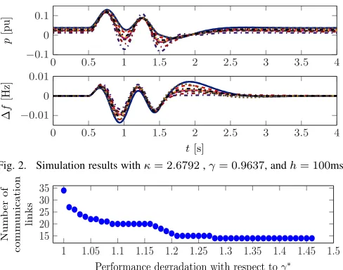
conducted in Matlab by using Yalmip [32]. This yields a nominal feedback gain ofκ= 2.6792 and a nominal bound for the L2-gain of γ∗ = 0.9637. The presented results in
Fig. 2 illustrate the convergence of the system trajectories to a synchronized motion after being subjected to external perturbations. The fast-varying delay is implemented as a piecewise continuous signal with a sampling time of2ms.
By taking these values as a benchmark, we redesign the controller with the aim of minimizing the number of communication links, while preserving delay-robustness. To determineWZ we employ the reweightedℓ1-norm, see
0 0.5 1 1.5 2 2.5 3 3.5 4 −0.1
0 0.1
p
[p
u
]
0 0.5 1 1.5 2 2.5 3 3.5 4
−0.01 0 0.01
t[s]
∆
f
[Hz
]
Fig. 2. Simulation results withκ= 2.6792,γ= 0.9637, andh= 100ms
1 1.05 1.1 1.15 1.2 1.25 1.3 1.35 1.4 1.45 1.5 15
20 25 30 35
Performance degradation with respect toγ∗
Nu
m
b
er
of
com
m
u
n
ic
at
ion
li
n
k
s
Fig. 3. Number of non-zero elements ofZfor different values ofγ. The number of required communication links in the case ofγ∗= 0.9637is 34.
Note that in all cases, robustness with respect to fast-varying delaysτ(t)≤his guaranteed.
Recall that the design approach leading to (IV.6) is based on the descriptor method with fixed tuning parameter ε. The latter could potentially introduce some conservativeness. Thus to improve our estimate of theL2-gain, we solve (IV.6)
and implement the obtained values forκandLin a modified version of the conditions for stability analysis derived in [15] that incorporates theL2-gain performance. The resulting
performance index γ with the analysis conditions in [15] is only9.5%lower than the γ∗ obtained via (IV.6). Hence, in
the present case the descriptor method does not introduce significantly more conservativeness, while providing the ad-vantage thatκandLare free design variables (in the analysis in [15] they are treated as constant parameters).
VI. CONCLUSIONS
Time delays and exogenous disturbances represent sig-nificant challenges in distributed control of MGs. In this paper, we have proposed a synthesis for a consensus-based secondary frequency controller in MGs that guarantees delay-robustness and simultaneously permits to trade off finite
L2-gain performance against the sparsity of the required
communication network. The design criterion is derived based on a LKF together with the descriptor method and cast as a constraint convex optimization problem. To enforce controller sparsity, we employ the usual reweightedℓ1-norm.
The presented case study on the CIGRE benchmark MV dis-tribution network illustrates the design trade-off between the number of communication links and the guaranteeable L2
-gain. In future work, we plan to validate our design criterion experimentally and incorporate voltage and reactive power dynamics and control in the analysis. Moreover, we will explore further applications of time-delay stability analysis and control design in MGs and bulk power systems.
REFERENCES
[1] H. Farhangi, “The path of the smart grid,”IEEE Power Energy Mag., vol. 8, no. 1, pp. 18 –28, january-february 2010.
[2] G. Strbac, N. Hatziargyriou, J. P. Lopes, C. Moreira, A. Dimeas, and D. Papadaskalopoulos, “Microgrids: Enhancing the resilience of the European megagrid,”IEEE Power Energy Mag., vol. 13, no. 3, pp. 35–43, 2015.
[3] J. Schiffer, D. Zonetti, R. Ortega, A. Stankovi´c, T. Sezi, and J. Raisch, “A survey on modeling of microgrids—from fundamental physics to phasors and voltage sources,”Automatica, vol. 74, pp. 135–150, 2016. [4] J. Guerrero, P. Loh, M. Chandorkar, and T. Lee, “Advanced control architectures for intelligent microgrids – part I: Decentralized and hierarchical control,”IEEE Trans. Ind. Electron., vol. 60, no. 4, pp. 1254–1262, 2013.
[5] P. Kundur,Power system stability and control. McGraw-Hill, 1994. [6] J. W. Simpson-Porco, F. D¨orfler, and F. Bullo, “Synchronization and
power sharing for droop-controlled inverters in islanded microgrids,”
Automatica, vol. 49, no. 9, pp. 2603 – 2611, 2013.
[7] A. Bidram, F. Lewis, and A. Davoudi, “Distributed control systems for small-scale power networks: Using multiagent cooperative control theory,”IEEE Control Systems, vol. 34, no. 6, pp. 56–77, 2014. [8] C. De Persis and N. Monshizadeh, “Bregman storage functions for
microgrid control,”IEEE Trans. on Automatic Control, 2017. [9] X. Wu, F. D¨orfler, and M. Jovanovi´c, “Topology identification and
design of distributed integral action in power networks,” inACC, 2016, pp. 5921–5926.
[10] E. Tegling, M. Andreasson, J. W. Simpson-Porco, and H. Sandberg, “Improving performance of droop-controlled microgrids through dis-tributed PI-control,” inACC, 2016, pp. 2321–2327.
[11] S. Lee, C. Lee, M. Park, and O. Kwon, “Delay effects on secondary frequency control of micro-grids based on networked multi-agent,” in
ICCAS, 2016, pp. 655–659.
[12] J. Lai, H. Zhou, X. Lu, X. Yu, and W. Hu, “Droop-based distributed cooperative control for microgrids with time-varying delays,” IEEE Trans. on Smart Grid, vol. 7, no. 4, pp. 1775–1789, 2016.
[13] E. A. A. Coelho, D. Wu, J. M. Guerrero, J. C. Vasquez, T. Dragiˇcevi´c, ˇ
C. Stefanovi´c, and P. Popovski, “Small-signal analysis of the microgrid secondary control considering a communication time delay,” IEEE Trans. Ind. Electron., vol. 63, no. 10, pp. 6257–6269, 2016. [14] C. Kammer and A. Karimi, “Robust distributed averaging frequency
control of inverter-based microgrids,” inCDC, 2016, pp. 4973–4978. [15] J. Schiffer, F. D¨orfler, and E. Fridman, “Robustness of distributed
averaging control in power systems: Time delays & dynamic com-munication topology,”Automatica, vol. 80, pp. 261–271, 2017. [16] X. Wu, F. D¨orfler, and M. Jovanovi´c, “Input-output analysis and
de-centralized optimal control of inter-area oscillations in power systems,”
IEEE Trans. on Pow. Sys., vol. 31, no. 3, pp. 2434–2444, 2016. [17] S. Schuler, U. M¨unz, and F. Allg¨ower, “Decentralized state feedback
control for interconnected systems with application to power systems,”
Journal of Process Control, vol. 24, no. 2, pp. 379–388, 2014. [18] E. Candes, M. Wakin, and S. Boyd, “Enhancing sparsity by reweighted
ℓ1 minimization,” Journal of Fourier Analysis and Applications, vol. 14, no. 5, pp. 877–905, 2008.
[19] E. Fridman,Introduction to time-delay systems: analysis and control. Birkh¨auser, 2014.
[20] K. Rudion, A. Orths, Z. Styczynski, and K. Strunz, “Design of benchmark of medium voltage distribution network for investigation of DG integration,” inIEEE PESGM, 2006.
[21] A. van der Schaft, L2-gain and passivity techniques in nonlinear control. Springer, 2000.
[22] H. K. Khalil,Nonlinear systems. Prentice Hall, 2002, vol. 3. [23] R. Diestel,Graduate texts in mathematics: Graph theory. Springer,
2000.
[24] C. Godsil and G. Royle,Algebraic Graph Theory. Springer, 2001. [25] J. Schiffer, D. Goldin, J. Raisch, and T. Sezi, “Synchronization of
droop-controlled microgrids with distributed rotational and electronic generation,” in52nd CDC, Florence, Italy, 2013, pp. 2334–2339. [26] J. Schiffer, R. Ortega, A. Astolfi, J. Raisch, and T. Sezi, “Conditions for
stability of droop-controlled inverter-based microgrids,”Automatica, vol. 50, no. 10, pp. 2457–2469, 2014.
[27] E. Fridman, “Tutorial on Lyapunov-based methods for time-delay systems,”Europ. Journal of Control, vol. 20, no. 6, pp. 271–283, 2014. [28] J. Hespanha, P. Naghshtabrizi, and Y. Xu, “A survey of recent results in networked control systems,”Proceedings of the IEEE, vol. 95, no. 1, pp. 138–162, 2007.
[29] F. D¨orfler, J. W. Simpson-Porco, and F. Bullo, “Breaking the hierarchy: Distributed control and economic optimality in microgrids,” IEEE Trans. on Control of Network Sys., vol. 3, no. 3, pp. 241–253, 2016. [30] J. Schiffer and F. D¨orfler, “On stability of a distributed averaging
PI frequency and active power controlled differential-algebraic power system model,” inECC, 2016, pp. 1487–1492.
[31] P. Park, J. Ko, and C. Jeong, “Reciprocally convex approach to stability of systems with time-varying delays,”Automatica, vol. 47, no. 1, pp. 235–238, 2011.
[image:7.612.56.300.50.242.2]