Applications of differential difference equations

A P P 1 I CAT ION S 0 F D IFF ERE N T I A 1

D IFF ERE N C E E QUA T ION S

A thesis submitted for the degree of MASTER OF SC IENCE

at the Australian National University, Canberra

by

Noel Gregory CRASKE

duly acknowledged, is original and was done during the course ,of this degree.

1.

PREFACE

This thesis was prepared under the supervision of Professor

A.

Brown. I am deeply indebted to him for his considerable guidance and his many helpfu~ suggestions. I would like to take this opportunity to express my thanks to him for this and the interest he has shown in my progress.

CONTENTS

PREFACE.

SID1MARY.

PART ONE _

DIFFERENTIAL DIFFERENCE EQUATIONS AND POPULATION GROWTH.

1. A MODEL FOR POPULATION GROWTH.

1.

4.

Introduction. 7.

Z'(t) = - 0 ( Z(t°o_ 1) (1 + Z(t))as a Population Growth Model. 11.

Comparison wi~h Population Data. 14.

Bibliography.

20. PART TWO _

A DIFFERENTIAL DIFFERENCE EQUATION FOR EPIDEMICS.

2. HISTORICAL SURVEY AND COMPARISON WITH RECENT WORK.

The Early Work. 23.

A Differential Difference Equation for Epidemics. 29.

Another Approach. 31 .

A Comparison with Recent Work. 33.

Approximations to the Differential Difference Equation.

39

.

3.

THE EPIDEMIC EQUATION. Preliminaries.

A Numerical Approach.

3

.

Calculating the constant c for A

=

O.

The Real Roots of the Characteristic Equation. The Complex Roots of the Characteristic Equation . Interpretation of Solution Types for A ~ O.

Susceptibles Leaving the Population (A

<

0). The Laplace Transform Solution.

4

.

APPENDIX.

Bibliography •

•

59

.

61.

65. 66. 69.

72

.

4.

SUMMARY

This thesis is divided into two parts, each

part examines an area in mathematics where differential

difference equations have arisen.

Part one considers an application to modelling

population growth, in particular the case of an animal

population which suddenly grows in numbers to epidemic

proportions and then falls off just as suddenly. Often

these sudden surges appear to recur periodically and the

modelling uses a differential difference equation whose

solutions show a similar behaviour.

Chapter 1 traces the development of this

differential difference equation, viz.

and describes how the parameter cr may be determined so that this equation can be used to represent a given set of data.

Tpe

research presented here may be considered as

supporting Mazanov's claim that this equation can be used

to model populations whose behaviour is of the type

described in the previous paragraph (Part 1, reference

9).

Part two examines in detail the development of

· 5.

relevant works of the past and inter-relates them. Much of this chapter is quoted from the appropriate references and its purpose is to provide the reader with a

comprehensive background on the subject, as well as to compare the results of earlier research with those obtained in the course of this project.

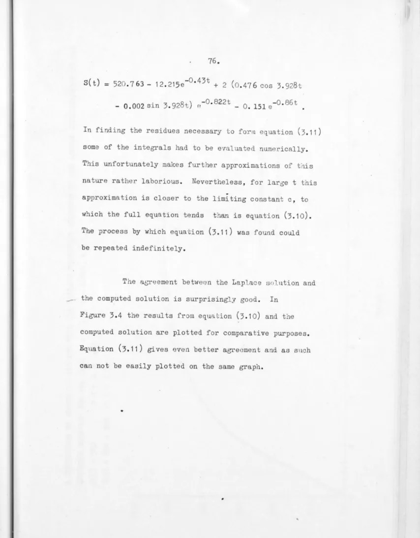
Chapter 3 centres on solving the differential difference equation for epidemics, namely

'A - S' ( t) = r S ( t) ( A G- - S (t - 7:) + S (t - "C' - G") ) , and determining the behaviour of the solutions as the parameters and initial conditions are altered. Particular emphasis is placed on the case when A = 0, as the behaviour ~ of the solution under this condition is not well documented.

For A

=

0, a method of calculating possible equilibrium values for S(t) is described, and the behaviour of S(t) under the influence of perturbations about the equilibrium positions is examined.

PART ONE

DIFFERENTIAL DIFFERENCE

EQUATIONS

AND

1. A HODEL FOR POPULATION GROWTH.

Intr oduc tion

A simple model of population growth is to consider the rate of growth as proportional to the current size, N(t), of the population, giving

oc

>

O.

h. () cx'( t-t ) From t 1.S, N t

=

N e O ,

o

where N is the population size at time t

=

t •

o 0

Equation (1 .1) models a population depicting pure exponential growth and does not have the flexibility to portray the

various growth changes which can occur.

A

more realistic model for the growth rate of a

population would be

(cx ,(3 ) O),

as this allows for the fact that the population may have a limit on its size owing to environmental restrictions (e.g. lack of food or space).

Equation (1.2) may be solved directly to give ( 1 ) •

-ext 1 + ce

N(t)

=

c constant.

The above models restrict themselves by assuming that the rate of increase of the population depends

entirely on its present size. Extending these basic models to differential difference equation form removes

this restriction by allowing the rate of increase in the population to be determined by the population size at times other than the present.

For example, equation (1.1) may be replaced by the following differential difference equation with. delay w

<X

>

O.

In order to solve equation (1 .1) it is necessary to know the population size, No' for some time to. To solve equation

(1.3)

it is necessary to know an integrable function which describes the behaviour of the population over a time

interval of length w.

Suppose N(t) _,

=

pet)

_,

From equation

(1.

3),

N(t)- N(O) =

-w ~ t

"

0

.

<X f :(T- w)dT,

for

and hence N(t)

=

<X

J

t~(u) _w du + N (0), for

o

~ t ~ w • But N(t) is known for this range of integration and hence

N

(

t

}

~

a.

J

t -w

-

-9.

Repeating this process reveals the behaviour of the model for 0 , t ~ nw', where n is the number of time intervals of length w for which a solution is required.

Similarly equation (1.2) may be replaced by

N'(t) = o<N(t-w)

p[

N(

t-w )] 2,

which may be further generalised ~o

where w

o' w1 and w2 are three distinct de,lays.

Let N(t) = ~ (Z(t) + 1).

Then N'(t) =~ Z'(t) and the equation becomes Z'(t) = -ex [Z(t-w

1) + Z(t-w2) + z(t-w1) z(t-w2)- Z(t-wo)}' (1.E

By choosing w

o' w1 and w2 appropriatel~ equation

(1.6) gives rise to two inte~esting equations.

Let w

₌

w₁

=

0 and _w2

=

w, then 0

Z let)

₌

_-

<X Z(t-w) (1 + z(t)), and let \oJ

=

W - wand w

2

=

0, then

0 1

-Z'(t)

=

-

<X Z(t) (1 + Z(t-w)).

Equations (1.] and (1.8) may be simplified by letting t = wt1 and

Z(t)

=

Z(wt₁)

= Z1(t

₁).

(1. 7)

Th _{en dt}

§M.li

~

dt w

Hence equations (1.7) and (1 .8) become

and

respectively, where cr₁ = <X w.

The works of Jones (references 5, 6 and 7) and

Cunningham (reference

3)

show that, depending on <X

1' periodic

solutions of equations (1.9) and (1.10) can occur. By

solving these equations over a number of intervals for

various values of cr

1 and a given initial function, it is

evident that the period and maximum value of the solutions

are functions of <X 1.

then, for w in years,

If the period for theoretical cr

1 is ~,

~w is the period in years when

equations (1.9) and (1.10) are considered as modelling

population behaviour.

In his discussion of equation (1.10) Cunningham

was primarily interested in comparing the solutions of

(1.10), which he obtained on an analogue computer, with

those obtained by approximating equation (1.10) by an

ordinary differential equation. He replaced the delay term

by the first three terms of a Taylor expansion and, using

11.

peak height and period of oscillation when

cr

1 was large. From his numerical work he found that sustained oscillations

did not occur in the examples he considered unless ~1 was greater than 1.8.

Wright, in his paper on equation (1 .9) (reference 11),

proves the existence of undamped oscillatory solutions for

a

1

>

11/

2

as well as the asymptotic stability of the zero solution for 0

<

cr

1( 1.5. Kakutani and r1arkus (reference 8) present theorems separating the monotonic asymptotic behaviour for 0

<

0(1

<

1/e and the oscillatory behaviour which occurs for 0(1 ) 1/e.

The properties of the solutions of equation (1 .9),

__ - as discussed by Wright and Jones,indicate that this equation

may be a satisfactory model for certa~n types of population

growth.

Zt(t) = -0( Z(t - 1) (1 + Z(t)) as a Population Growth Model.

The subscripts of equation (1.9) have been dispensed

with and toe delay taken as one year.

The condition Z

= 0 corresponds to

N = cr/~ and

Z

=

-1 corresponds to N = 0 , as can be seen from equation (1 .5). Thus

Wright has shown that for ex

>

1/e and Z(O) - 1 there is

no solution ,'whi'ch' approaches zero monotonically as t

becomes infinite, and that there exist non-constant

periodic solutions for all ex

>

1i /2, with Z(t) bounde~i.

Mence using (1.9) as a population growth model means that once

the initial population is established, with Z(O) -1, it will

continue in an oscillatory fashion, the amplitude and

period of oscillation most likely being det~rmined by the

environment.

Jones has shown that for ex

>

-rr/2 the solutions,

for various initial functions, tend to become periodic and appear

~to be identical within a translation along the ti~e axis.

Hence for convenience of calculation the initial function

on -1 ~ t " 0 may be chosen to be Z( t) = t.

The oscillatory properties of the solution vary

markedly wi th ex. For ex near 11'/2 the solution is

virtually sinusoidal, which may be thought of as modelling

smooth changes such as seasonal changes in the size of

some population. However, for large ex the solution has

the appearance of periodic high peaks separated by long

troughs of size hardly greater than zero (i.e. Z(t)

slightly greater than -1). Such a solution provides a

13.

vole population sizes and other phenomena where populations

increase rapidly after long periods of quiescence, to

epidemic proportions, and vanish just as suddenly as they

appeared. Further, when ~ is large, the solutions have

another important property in common with the real life

examples - they are not symmetrical about the population mean.

In order to compare numerical solutions with

known data a co~on baseline and common scales on each

axis are necessary. The most natural baseline appears

to be the mean, i.e. that line about which the areas

under the solution and data curves are equally distributed.

To explain this remark:

let a periodic solution! of equation (1 .11) have period T.

Then z( t+T)

=

Z( t) for all t

>

t _o , where t is that 0

period of time which must elapse before the solution

becomes periodic.

From Z'(t) = -CJt

(1

+ Z(t)) z (t -

1),

+

z(t2)

1 + z(-t

1)

side becomes 1.

Hence

= exp ( - ~

=

J

t 2 -1 Z( u)du) • t -1

1

z(t

1) and the left hand

'14.

Thus the integral over one period is zero, i .e. the mean

is Z = O.

Solutions of (1.11) range between -1 and a

maximum value determined by~. A program based on the

method outlined by Jones was used to generate solutions to this equation.

The graph of Z against ~ (Figure 1.1) was

max

obtained by varying ~ and noting the upper limiting

value of the numerical solution after several oscillations. The use of this graph provides a convenient method for determining that ~ for which a solution of equation (1.11)

--

will represent given data.

Comparison with Population Data

Fox fur numbers taken by the Hudson Bay Company and by Moravian Missions in Labrador, as presented by C.S. Elton (reference 4, pages 265 and 313), serve as

good sample data (Figures 1.2 and 1.3 respectively).

Only a segment of the data has been graphed as

this is sufficient to demonstrate the concept. For the

1872-1925 data, the closure of the Zoar post in 1888 has

not affected the periodic nature of the data, and so the

discontinuity has been' ignored. The furs taken from ZOGr

Z

max

4

3

2

1

o

15.

z'(t)

=

-

ocZ(t-1)(1 + Z(t»

PERIODIC SOLUTION MAXIMA

FOR VARIABLE

oc.

oc

1 2

3

16.

may have been sent to Davis Inlet, although Nain was

closer. In comparison with other stations, Zoar's

contribution of furs was generally low, so its closing

would not be very noticeable. The average maximum annual

number of furs, D , and the average minimum, Do , for

max mln

this set of data are 253.9 and 62.6 respectively, while

the mean, D _mean , is 149.3. In terms _tOO of the periodic

solutions to (1.11) the distance between the mean,

Z

=

0, to the minimum value, Z(t)

=

-1, corresponds to an interval of 149.3 - 62.6 i .e. 86.7 in the original data. Similarly the distance from Z = 0 to the peak

height, Z in the solution of (1.11) corresponds to max

253.9

Thus

149.3 i .e. 104.6 in the original data.

Z

max

1 =

D - D 104.6

max mean

= _ 1.21.

D D 0 86.7

mean mln

Similarly, for the 1845-1910 data

Z

=

max

631.0 - 311.9 31 1.9 - 75.9

The Z values for the data sets are sufficiently • max

close that the values of ~, as read from the graph (Figure 1.1),

are virtually identical. The table from which the Davis

Inlet, Zo~ and Hopedale graph was constructed was

inserted by Elton to show that there was no essential

17.

sources in the same region. The virtually identical ~

values support this claim. Taking ~ = 1.87 gives a

reasonable fit for both sets of sample data (Figures 1.2 and 1.3).

For the 1845-1910 data,Elton believma phase

change occurred in the late 1890's. There does appear

to be a shift in the peaks but the numerical solution

does not support the claim of a complete phase change.

Thus the equation Z'(t)

=

-~ Z(t-1)(1 + Z(t))

appears to provide a good model for the growth of

300

\

2001 1'1,

Ul

\ ! \ I

a: ::J LL X 0 LL

100 l- II

_'!..1

?

1870

I \

I'

,

I,

I' _I,

I I'

I I

,

I

,

I

.1 /I , I

I '

I _I

,

I

I

\\I!\ \

A

I

'(\

I

~

)

~~;

~

, ,,~

,

I' I'

zo ....

CLO,J~l)

1880

L 1890

I

\

I I I I I

I

I /

V I 1 \ \

,

\

~

II

1900

YEAR

,

I \ \ \1 V

ColOllred fox fur returns from DavIS Illlct. ZOJr. Hop, ' Ie: 1872 - 1925

1,'1< ;(1 HJ·; 1.?.

1\ .1 I \ I

,

I

,

I

\ 'J

, I

V

1910

L

I I

,

I ,

,

,

_ _ ACTUAL FUR RE ruRNS

____ NUMERICALLY I'REDICrED

FUR RETURNS

Dmax 753.9 I'. Ii

I I I,

I I, 'I

II 1\ , /1 II I Drncan 149.3

~"

')

\

~;

r

, I _{V Din'"}

62.6

1920

1200

I

_ _ ACTUAL FUR RETURNS

1000 I- ~JUMERICALL Y PREDICTED FUR RETURNS

Vl

a: :J u.

'T

::

J\

/:\,

_IJ

I

_I

,I

A

I "I i

I

\

I

I.

I\//~r

700 t'-1

Ii

_V'

_wV

J

_\J

V

II \/, ,

'\

I

¥ ' ,

•

01 I .1 _ _ I

1850 1860 1870 1880

YEAR

Fox fur rel,,,ns from LJorador Missions: 1845 - 1:3 10

FJGURE 1.3

,,1

j -1890

Dmax = G31.0 Dmea" = 311.9

Dmi,,'= 75.7

, \ , \

I ' \ \ I

\ ,

1\

I I

\

,

1900

1..0

20.

BIBLIOGRAPHY

1. BELLMAN, R. and COOKE, K.L.

"Differential-Difference Equations".

Academic Press, New York, 1963.

2. CRASKE, N.G.

"A Population Growth Model".

Search, Vol. 5, No. 6, 261-263, 1974.

3. CUNNINGHAM, W.J.

"A Nonlinear Differential Difference Equation of Gro,.th".

Proc. Nat. Acad. Sc., Vol. 40, 708-713, 1954.

4. ELTON, C.S.

"Mice, Voles and Lemmings".

Clarendon Press, Oxford, 1942.

5. JONES,G.S.

"On the Nonlinear Differential-Difference Equation

f '(x) = - exf(x-1)(1 + f(x))".

Journal of Math. Anal. and Applications, Vol. 4,

440-469, 1962.

6. JONES, G.S.

"Asymptotic Behaviour and Periodic Solutions of a

Nonlinear Differential-Difference Equation".

Proc. Nat. Acad. Sc., Vol. 47, 879-882, 1961.

7. JONES,G.S.

"The Existance of Periodic Solutions of

f '(x)

=

-

ex r(x-1 )(1 + f(x))".

Journal of Math. Anal. and Applications, Vol. 5,

435-450, 1962.

8. KAKUTANI, S. and HARKUS, L.

"On the Nonlinear Difference-Differential Equation y I (t) = (A - By (t -

£.)

)

y (

t)

" .

Contributions to the Theory of Nonlinear Oscillations IV,

Annals of Math. Studies, No. 41 , 1-18, 1958.

9. MAZANOV, A.

"On the Differential-Difference Growth Equation".

21.

1

0

.

SLOBODKIN, L

.

B

.

"Growth and Regulation of Animal Populations".

Holt Reinhardt and Winston, New York, 1961.

11.

WRIGHT,

E.M.

"A Nonlinear Differential-Difference Equation".

PART TWO

A

DIFFERENTIAL

DIFFERENCE

-23.

2. HISTORICAL SURVEY AND COMPARISON WITH RECENT WORK. The Early Work

Soper's approximation to a continuous epidemic

considered a community into which there was a continuous

flow of susceptibles (reference

3)

.

Within the community there was assumed to be

(i) an equal susceptibility '~o the disease prevalent in the community,

(ii) an equal capacity to transmit the disease according to a law when infected,

at the end of the infectious period, after being cured, persons were no longer susceptible.

Further, either the disease is acquired as the

result of over-accumulation of doses of infection above what can be dealt with by the resisting powers of the body or it is acquired instantaneously. After acquisition, the disease has powers of infecting others according to some law of intensity over an interval of time, or there is an incubation period at the end of which all infecting power is

concentrated.

Soper was primarily interested in epidemics of

24.

point or instant infection at the end of an incubation

period.

Let x be the number of susceptibles at time. t

and let m be the "steady state" number of susceptibles, i.e. the number necessary for one old case to produce

exactly one new case. If we assume that the number of

.

susceptibles infected by one case is proportional to the number of susceptibles in the community at that instant, then x/m cases will arise from one case at the

end of the interval.

Soper now considers m

=

sa where a is the number of susceptibles recruited into the population in unit time to give the steady state m. Hence s may be considered as

a measure of the "seclusion of the community", a large value of s indicating that there are few interactions of the sort

which produce infection.

Taking the incubation period as unit time and

z~ as the number of cases in the interval succeeding a

particular instant and Z

_-,2

11. as the number of cases in the preceding unit interval, then

= _m x Z

-,2

11. •

.

.

25

.

Epidemic curves were produced taking a = 1000

and s = 20, 30, 40, 50, so that the steady state numbers of susceptibles were 20,000, 30,000, 40,000 and 50,000.

Soper began his calculations with the initial condition

=

z

-

Yz

which occurs at a peak, and hence x

=

m. The successive values of x were obtained by adding 1,000 susceptibles each time and subtracting the number of cases in the preceding interval.

The curves obtained appear to repeat themselves

precisely with no damping. Later work by Soper indicates that

damping of successive peaks is to be expected only when infecting

pOlo1er lasts for a finite time. Hence when instant infection is

considered there can be no damping.

Taking- the incubation period as 7:

,

then ZY2 'C x

J:<a

=

and since x

₌

m + - Z) dt ,

Z m

-Y21:'

Xl = a - Z •

Time t is taken from an instant when susceptibles are level, namely at a peak. Soper now proceeds to find the period for small epidemics as follows:

26.

index measure of cases. If u is assumed to be small

then Z = a(1 + u) and x I = -au.

Also _{ZYz~ = a(} 1 + u +

Yz

Tu I)

and Z

-

Yz

'l'

= a(1 + u - Yz-cu ') ,

Hence x/m ₌ 1 + 't"u ' - 1 + ~u'

1 + u

or x - m = m 1;" u ' = sa _{(;" u' .}

From equation (2.2) sa't"u" + au =

0,

which has solution

au = F cos(nt + g) with n2 = 1/s1:' and F,g constant.

Hence Z - a = F cos(nt + g) ,

and x - m = (F;fl ) cos (nt + g + 1l'/2).

Z

The initial time is taken when;(is at a maximum

and hence g = O. Therefore Z - a = F cos nt ,

and x - m =-(F/n) sin nt •

~e cases curve, given by equation (2.3a), and the susceptibles curve, given by equation (2.3b), are 11/2

out of phase. The curves take the form of small sinusoidal

oscillations with the cases curve lagging behind the

susceptibles curve. The period of small epidemics is

27.

For more general epidemics Soper noted the

following features of the curves. 1 )

2)

4)

The cases curve follows behind the susceptibles

curve, and cases are at a peak when

susceptibles are decreasing from the steady

state value m, and at a minimum when the

susceptibles are increasing from the steady

state value.

For small oscillations the lag is a quarter

period.

Susceptible numbers are maximum when the cases

are on the increase from the steady state value

and are minimum when the cases are on a decrease

from the steady state value.

The time for susceptibles to rise to a maximum

is much greater than that to decline to a

minimum unless the oscillations are small. If the rise and fall times be taken to the extreme

the susceptibles curve is saw-tooth shaped.

When peaks are immense, that is the epidemic is

explosive, there follows a long intermission when cases remain few, and the susceptibles rise

uniformly at the rate of accession of new

6)

While the susceptibles are rising at a

uniform rate the equation of the cases curve is

m + at

m and the curve is trough shaped.

Initially Soper considered only that the

infecting power was concentrated at the end of the

incubation period. In his appendices he discusses

the more general case where the ability to infect starts

from the moment infection takes place and lasts for the

entire interval " • The resulting curve has the form

of exponentially damped oscillations. Soper found the

period for small epidemics as follows:

If ~ is the length of the infection interval

then the chance that recovery may occur at any instant is dt

~ If y is the number of infected individuals at any

moment then

"recoveries".

y~ is the depletion of y in time dt due to

t"

Then in the steady state, if a is the number of

accessions,a is also the number of new cases. Therefore

y = a ~ and x = as. At any moment the new cases per unit

time are ~

I-

.

Hence the equations for developing the as at"

epidemic form are

x, _{= a}

_-

_a-x _-Y

as at'

29.

If u and v correspond to small depa.rtures in x and y

from their steady state values as and a~, respectively, then

x ..L

putting as

=

1 + u, a~

=

1 + v and neglecting products

of u, v we get

su' = - u - v

1;: v , _{= u}

u" + u' _s +

-

u =

s't:

with the same equation for v.

-t

0

2

1)

~

,

t )

The solution is u = Ce s cos

L

1 -

4s

Ts'i-

J

for C constant.

Thus the period is now and it will be slightly

longer than the period 21'(

&'

found for the "point"

hypothesis. The constant of damping is 1/2s.

A Differential Difference Equation for Epidemics

Soper's approach can be extended to give rigorous

equations for a theory involving the basic concepts of

epidemics through the tran~mission of disease as follows.

Let I (t) and S(t) be the numbers of infec~ious

persons and susceptibles respectively. The rate of loss of

susceptibles, dt dS ' is equal to the rate at which

susceptibles become infected, C(t), less the rate of

30.

The rate C(t) is proportional to the product

of ret) and Set).

The newly infected persons C(t) dt become

infectious after a latent time ?;" and remain infectious

for a time G'-' In effect the two possibilities

considered by Soper initially have been combined. rf ~ is small the equations represent point infection, while

if ~ = Q the infecting power is possessed immediately

infection has taken place and is exercised without loss until the moment of recovery.

Hence -S'

₌

C(t) - A( t) , C(t)

₌

ret) ret) Set)

r-~

ret)

₌

C( t) dt •

t -T-G"'

The factor r and the rate of recruitment A are generally taken as constant, though Soper shows that r (which is related to m) has a seasonal variation.

Taking r and A as constant, the variables C and r may be eliminated to get

A - S' = r S (Ae;- - S (t - T ) + S (t - '1: - a-))

(2

.4)

31.

to m, equation (2.4) yields r G- S = 1, that is r G- m 1,

for A ~ O. Hence r (S' is the inverse of m.

Tn terms of this notation the discrete equations

developed by Soper are

1. _1.+ 1 S_1. . =

1. m

1.

and _{S. 1 1+} = S. _1. I + A i+1

where I. and S. are the infectious cases and the susceptibles 1. 1

in the i th generation respectively. The length of each

generation is taken as the incubation period, that is ~ = 1. In the stationary condition S.

=

m, I. 1

=

I ., S. 1

=

S.

1. 1.+ 1. 1.+ 1. and I. 1 = A.

1.+

Another Approach

Wilson and Burke reference unpublished lectures presented by Dr . W.H. Frost at Harvard Medical School in 1928. The following extract from Wilson and Burke (reference 5) outlines Frost's approach:

"Frost considered that for the diseases to

which his theory would be applicable one could think in

terms of generations of infectious persons Ii who being

in contact with susceptibles S. for a certain period would

1.

infect some of them who would then become the new

32

.

by the 'incubation period'; but he recognised that in

the intermixture of susceptibles and infectious some

of the susceptibles might have multiple contacts with

infectious persons and yet could develop at most only

one infection apiece. If S. were the number of

~

susceptibles, p = 1/S. would be the chance that any

~

particular contact would fall upon any particular susceptible and q

=

1 - 1/S. would'be the chance that

~

he would escape. If then there were k. contacts made ~

between infectious and susceptibles the chance that a k i

susceptible would escape them all would be q and the

chance that he would have at least one contact would be k·

1 -

q~.

The number of infected would therefore be

k·

--·S. (1 - q ~). Frost assumed that the number of contacts

~

k. would be proportional to the numbers of infectious

~

and of susceptibles jointly, or k. = rIo S. . Thus his

~ ~ ~

equations corresponding to Soper's equations

(2.0a)

and (2.5b). are

rIo

Si }

[ 1 1

~

1. 1 = S. - (1

-s.-

)

,

~+ ~

(

2

.

6a)

~

and _{S. 1} = S. _{- 1. 1} +

A

~+ ~ ~+

(2.6b)

33

.

of the curve of an epidemic so sharp that the number

of recruits during the epidemic would not materially

influence the course of the epidemic."

A Comparison with Recent Work.

Wilson and Burke proceed to demonstrate that

the theories of Soper and Frost have a lot in common.

If I. and r are sufficiently small then only the first

1

two terms of the expansion of (1 - 1/S.)rIi Si need be

1

considered. Consequently equation (2.6a) becomes

1. ₁₊ 1 --S i (1 - (1-r1.» 1 = r1. 1 S. 1

and since r = ~ equations (2.5a) and (2.6a) are identical. m

In terms of the differential difference equation (2.4), r

in Frost's theory is equivalent to r ~ This is to be

expected because the rate of new cases in each equation

must be the product of a contact rate r by a time

available for making contact.

In order to make the computation of equation (2.6a)

easier, Frost used the approximation

(1

₌

e -rI

assuming the number of susceptibles did not decline too far.

Hence

and

1. ₁₊ 1 =

-r1.

S. (1 _ e 1)

1

S. 1 = S. - 1. 1 + A

34.

In equation (2.7b) let A = O. _{Then I. 1 = S. - S. l '}

1+ 1 1+

Substitution in (2.7a) gives

-rS. -r S. 1

-rSo S. 1 1+ e 1 = S. 1 e 1- = = S1 e

i.e. S. 1 = _S1 exp r (S. S ) _(2.7c)

1+ 1 0

When the epidemic is ove~S. 1 and S. are equal

1+ 1

and constant, say c.

-rS -rc

S1 e 0

ce c =

-'rS -x

rS 1e

0

where

or xe = x = rc

.

(2.8a)

The corresponding relationship from the differential

difference equation, as will be derived, is

...

-x -ra'm

xe

=

r c;- oc e

-where x = r ~ c , m is the initial number of susceptibles

and oc the number one generation later.

However r~ for the continuous case is equivalent

to Frost's r for the discrete case.

Further, Sand m represent the initial number o

of 6usceptibles while S1 and oc are the number of

susceptibles after one generation. Hence equations (2.8a)

and (2.8b) are identical. In other words, the number of

35.

susceptibles remaining from an epidemic described by the

differential-difference equation is the same as that for

an epidemic described by Frost's equations. However, for the case examined (see Table 2.1) the duration of the epidemic is one generation longer and the curve has

a more negative skewness as described by the differential difference equation.

Table 2.1 shows the course of an epidemic as

predicted by the differential difference equation

(2

.

4)

compared with the results obtained by Wilson and Burke, using equations (2.5), (2.6), (2.7) (reference 5, page 363). The initial number of

-susceptibles was S

=

m

=

2000, and one infectious case

o

was introduced into the population, giving I _o = 1 or <X = 1999. The contact rate r was taken to be .001, Hence Soper's

m was taken as 1000, and G- was taken as 1 for the continuous

case. The generation period for the case of the differential

difference equation was taken as ('t' + 6"'/2), to be consistent

with Wilson and Burke. This generation period was used by Wilson and Worcester on the assumption that G- was small

(reference

6

).

It is also implicit in Soper's use of the notation Z 1, Z1 where he considers the incubation

-"2 "2

period as unit time and Z1 as the number of cases in the

"2

interval succeeding a particular instant. For the case at hand G'"

=

1:'

=

1. Consequently <i cannot be considered as

36.

TABLE 2.1

Course of Hypothetical Epidemic, I _o

=

1, S

=

2000, 0

r

=

0.001, showing numbers infected in each generation.

GENERATION EQUATION(2.5) EQUATION(2.6) EQUATION(2.7) EQUATION(2.4)

1 2 2 2 2

2 4 4 4 4

3 8 8 8 8

4

16

16 16 15

5 32 32 32 30

6 62 61 61 58

7 116 111 111 107

8 204 186 186 181

9 317 267 268 264

10 ₃₉₃ 308 309 308

11 332 265 267 270

12 171 173 173 177

13 59 90 89 93

14 17 41 40 43

15 5 18 17 19

•

16 1 8 7 8

17 3 3 4

18 1 1 2

19 1

Total Infected 1739 1594 1594 1594

Residual

37

.

Wilson and Burke obtain from equation (2.7) a

very neat result for the relationship between S / m, the

o

ratio of initial susceptibles to m = 1/r, and S~m, the

ratio of the residual susceptibles to the same number.

From equations (2.7) with A = 0,

1.

_l+ 1 = S. _l - S. 1 _l+

N N-1

Hence

L

1. =

L

(S. S. 1) = S _{- SN •}

J l l+ 0

j=1 i=o

Also ₌

1.

₁

l+ = S. l - S. 1 l+

Hence S. 1 = S. exp ( - r I . )

l+ l l

In particular = S exp ( -r I )

o 0

If

and

From equation (2.7c)

I. =

l

S. 1 _l+

o

for i

consequently

N

L

I.

i=o l

=

=

~

=

S1 exp ( - r

S exp ( - r o

N + 1, then

L:1.

_{. l} = l=O

i

Z I.)

j=1 J

i

.L

1.)

j=o J

SN = SN+1

S _{- SE ·}

0

Substituting into the previous equation for Si+1 gives

N

SE _SN+1 = S ₀ exp ( -r

L

1.)

,

i=o 1

S exp ( _{- r (So - SE»}

.

0 Hence

or

SE exp ( - _rSE) = So exp ( - rS

o) , rSE exp ( - rS

E) = rSo exp ( - rSo) •

This equation is almost identical with equation (2.8a). F = rS _o and f = rS

E, then

Fe -F fe -f •

This equation clearly has f = F as one solution. The

equation y = xe -x has maximum value y( 1) = 1/e. For x

>

0 and x ~ 1 two solutions for y exist. The consequences of this

are discussed further in Chapter 3. Presumably Wilson and

-F

I

Burke used cases where Fe

<

1 e, so that a solution

---could be found ,with f2

<

F for the second solution, f 2•

A table of corresponding values of f and F was

computed by Wilson and Burke (reference

5

,

page 364). We

have seen that equations (2.7), under the prescribed

conditions, approximate equation (2.4) very closely.

Hence, if r is replaced by r~ in the above analysis it

should also apply to the continuous case.

For the example in Table 2.1., So = 2000, SE = 406

and m

=

1/rtr

=

1000. Hence F = 2, f

=

.406 and f/F = .203.

39

.

Hence, given S , r and CO; from which F = S /r G"" can be found,

o 0

the table of Wilson and Burke provides a quick reference

to the approximate numbers of susceptibles remaining after the epidemic, provided the number of infectious

cases initially introduced into the population is not too

great.

.

Approximations to the Differential Difference Equation.

Two years later Wilson published two more papers,

this time with co-author Jane Worcester (references

6

,7

)

.

The two papers

were conc~rned with obtaining approximations to equation (2.4)

which could be handled by the computing equipment

available at that time. They considered several methods of approximation and it is interesting to compare the results they obtained with the exact solution.. Their first

approximation was to expand the right hand side of (2.4)

by Taylor's Theorem about t = -( ~ + a-/2). This gave

A - S' ( t)

=

r G- S ( t ) (A - S' (t - ~ -

u-

/2)) • This expansion was based on Soper's assumption that the time

of infecti<?usness G-' was so short that deri vati ves higher than the first could be neglected, giving Soper's "point" infection condition. However, it turns out that the exact solution of equation (2.4) which corresponds to the

examples considered by Soper has ~ -

.

1 and hence this

4

0

.

In the steady state S is constant and equal to

1

Introducing x = S/m transforms equation (2.9) to

m =

rc-A/m - x' = x(A/m - x'(t - '"z: - (;""/2» . (2.10)

If 7: + G""/2,which is Soper's "incubation period", be introduced as the unit of time and t, A and x are

transformed by t = T( '1:' + G""-/2), A1 = A( '1::'" + G""'/2) and

x 1(T) = x(t) respectively, then equation (2.10) becomes

In what follows the suffixes have been dropped.

Z

=

A/m - x' and u

=

in Z are now introduced in

place of x. As with Soper's work,u may be considered as an

index measure of cases. Equation (2.11) becomes

Z (T) = x Z (T 1) ,

or u (T) = in x + u (T - 1)

Differentiating equation (2.i2a) gives

u'(T) - u'(T - 1) = x'

x

But Z = A/~ - x', therefore

x'

=

~

(A/m _ Z(T» and by equation (2.12)

x x

x'

- -

=

x

Z (T -1)

Z (T)

However, Z

=

eU and hence

(A/m - Z (T» •

u(T)

e

]

.

(2.11)

41.

Substituting this equation in equation (2.13) and shifting the time

origin by 1 unit gives the result of Wilson and Worcester,

namely

u'(T + 1) - u'(T) = _

[1

_[A/m]e-u(T +

1)

J

_e u(T)

Equation (2.14) corresponds rigorously to Soper's

assumptions. Wilson and Worcester.noted that Soper had

effectively replaced the left hand side by the first term

of the expansion

u'(T+1) - u'(T) = u" + 1

2

1

u'"

+

6

u (iv) + • • •

and on the right hand side, since he is only dealing with

u(T) - u(T+1)

small epidemics, he has replaced e · by 1 as

~though u(T) and u(T+1) did not appreciably differ, giving

u" = _ (e u _ Aim) •

Wilson 'and Worcester then obtained and compared the

solutions of equations (2.14) and (2.15) when A = 0, namely

u" = _ eU _{and u' (T+ 1) - u} ,( _T) = ~ e u(T) •

The solution of the first is

u = 2 ln sach

fZ72

T + ln Z ,

o 0

or Z

=

Z se.ch 2 .; r Z

12

• T,

o 0

where Z is the rate of new cases at the peak, which is

o

taken as the origin of time. With A

=

°

and Z

= -

x', on integrating Z we have

(2.14)

x

=

x

o

/2Z

o

42

.

tanh

J

Z /2 ' T ,

o

with x _o being a constant.

Equation (2.17) provides us with a quick approximation

to the exact solution for specific examples. Consider the

previous example with the initial number of susceptibles

S _o = 2000, U- = ~ = 1 and r = 0.001, which left 406

susceptibles unaffected by the epidemic. Consequently, for

T large and positive

x = .406 and tanhJ Z /2' T = 1 •

o

while for T large and negative

x = 2 and tanh jZfl'T' = -1 •

o

Hence (2.16) gives rise to two simultaneous equations

and

From these, Z = .318 and x = 1.203 •

o 0

From column 4 of Table 2.1, the value of Z for the exact

o

solution is .308, from which it is seen that the above

approximation to the solution is reasonably close. Presumably

Wilson and Worcester did not realise that the constant

could be determined directly from the initial and final

43

.

From equations (2.12) and (2.16)

Mll

h 2 ;-:;::;; T

x( T)

=

Z(T _

1)

=

_s_ec

---:::---====:--sech2

~

(T - 1)

o

They noted that regardless of the value of the constant of

integration in equation (2.17), equation (2.17) and the

above equation for x (T) are not the same and they ascribed

this discrepancy to the hypothesis of Soper that the

epidemics under consideration are so moderate that higher

order terms could be neglected.

A better approximation for the case A

=

0 was

obtained by examining approximations to the solution of

ul _{.(T + 1) - u}l _{(T) = _ eu(T) •}

Assuming that u and a

=

ul(T) are known at any time T, the

o

value of u at T + 1 along the tangent to the curve is u + a. o

---From equation (2.18) the slope of the tangent at T+l is a_euo and 0. l,'''1! o-t t'h.5 slope. u proceeding from T to T + 1 along this line gives u + a _ eO .

" 0

Equation (2.19a) approximates u (T+1) by the mean of these

values. Equation (2.19b) is similarly obtained by considering T - 1.

u (T + 1)

and u (T - 1)

u (T) + ul

u (T) - ul

(T) -

t

eu(T) ,

(T) _ .1 eu(T- n

2

Equation (2.19a) was used for successive positive integral

values of T and equation (2.19b) for successive negative

integral values of T. Any intermediate values can be filled

in by using the parabola

u (T +

$)

= u (T) + u

l _(T)<&

44.

The next method they consider is approximating u by a series whose coefficients are to be determined. The

series expansion for u was taken as

'u=u +aT +

o +

where u

=

u and u'

=

a are known. After substitution in

o

equation (2.18) and solving for the coefficients up to

T~

we get

=

"t

==

S

₌

t:

=

u

e 0 (a2 _ 6a + 12) 2 (12 + eUO)

Z.

3 u ~ 24 u 0 0 .L 20 u u

(ae 0 _3e 0 6)

-

-

~

(2

P

(

't

U_o 12 + e

- 3ar

+ a~ +

3

0'

.1.

_{a 3 )} 6

2

_{_}

_.1.

a3)

+ a 2

(

eS

is given incorrectly with opposite sign in reference

6

,

page

44)

.

Another method considered is that of modifying

u" - eU to be a better representation of equation (2.18). We can

write

As an approximation, let _ eU

=

u" +

.1.

u'"

2

45.

Then _{- u' e}U = u"'

U_Slng · th' _{lS equa lon}t . _,

.1.

_{6 u}

(

i v) _may b _{e replaced in the higher}

order approximation to give

e u =

i

u"' + U" -

-t

u' e u

Ignoring the u"' term and differentiating, we get

II,

_u'eu = u

.1. ( ,)2

_{u e} u _•

3

The u"' term which was previously ignored may be replaced

by using this equation.

Hence

u

~ u'

2 +.

~

18

(u,)2

u

- e

If p = u " wi th the initial condition p =

o

when

u = _{uo '} we can integrate equation (2.21), giving

u

-

1}

u

-

1}

2

+12{1

8

+eu

_O

[

1

8

+

0

36

e

p p

-u

18

+

e 18

+

e

which may 'be Solved for p and integrated to give

.1.

_+.1.

_j

,

-1

)1

T ₌

₆

In (Z/Z ) 1

+

18/Z tanh - Z/Z

0

-

3

0

where Z is the case rate at the peak of the epidemic and T

o

is measured from that time. The + sign is u,sed for T

>

0

and the - sign for T

<

O.

(2.21 )

=

o

,

46.

Wilson and Worcester also noted that equation (2.21) may be

solved by an iterative process as

In(Z/Z) = 2 Is (aT - ~ Is (aT - ~ Is (aT - etc))), (2.23)

where Is stands for In sech and a for 3/

J

1 + 18/Z o.

o

The first four columns of Table 2.2 were computed

.

from the methods of approximation discussed by Wilson and

Worcester for the initial conditions Z

=

.308 and ZO(T)

=

0 o

when T

=

O. These initial conditions make a

=

0 in

equa tion (2.,20), and hence greatly simplify the expressions

for

(3,

r

'

~ and

G •

TABLE 2.2

Values of the case rate for some values of T.

T EQUATION(2.16) EQUATION(2.19) EQUATION(2.20) EQUATION(2.23) EQUATION(2.4)

o

-1 2 -2 3

-3

4 -4 8 -8

.308 .308

.265 .264

.265 .269

.176 .170

.176

.

.187

.098 .088

.098 .11 2

.049 .040

.049 .062

.002 .001

.002 .004

.308 .308 .308

.264 .2fl+ .269

.268 .267 .264

.168 .168 .177

.190 .185 .181

.068 .086 .093

.132 .110 .107

.041 .039 .043

.119 .061 .058

• NOT .001 .001

47.

As can be seen, the approximations correspond very

closely to the exact solution when the initial susceptibles

are 2000 and one infectious case is introduced, as previously

considered. Consequently the approximations appear to be

justified for the case at hand. For ease of comparison,the

above solution curves are graphed in Figure 2.1.

There is very little difference between the

approximations and the solution of equation (2.4) for the particular data tabulated. The skewness as measured

by the ratio of the third moment to the cube of the standard deviation is about - 0.33.

Hence it can be said tha~ these approximations for the examples considered are very good.

In a subsequent paper (reference 7) Wilson and

Worcester pointed out that equation (2.22) can be used to

give x as a function of Z, thus improving the approximation

given by equation (2.17). We can write

x - Xo = -

J

Zdt = -

J

Z

(-1!

)dZ •

From equation (2.22),

~~

=

iz

+

iz

J

~o

:

~

8

o

and hence

J

z

(dT)dZ _dZ

1.

₆ (Z - Z )

_±

t

J

_{(Z 0 + 18) (Z} - z)

0 0

Thus _{x -} x ₌

i

_(Zo-Z)

+

t

J

_{(18 + Zo) (Z - Z)}

A CO

MPARISON OF THE NUMERICAL SOLUTION OF THE EPIDEMIC E

Q

UATION WITH SOLUTIONS OBTAINED

BY

VARIOUS

METHODS

OF APPROXIMATION

FOR THE

INITIAL CONDITIONS

Z

=

.308

AND Z'(T)

=

0

WHEN

T

=

O.

o

EQUATION

(2.4)

CAS

E

RATE

Z

EQUATIONS

(

2

.2

3)

, (2.19)

EQUATION (2.20)

~

--- -. .;;y

--- ----p

/./.:

/.

~

~

,..

/~ ~

1--

4

_-3

-2

• 2

.1

-1

o

FIGU

RE

2

.1

- - x - -

E

QUATION

(2.16)

1 2

₃

T

4

.po

OJ

49

.

where the positive sign applies before the peak of the case

rate and the negative sign after it.

Equation (2.24) may be used to calculate the

total number of cases which occur durjng the epidemic.

Before the epidemic (T large and negative) and after the

epidemic (T large and positive) the case rate Z is zero.

Consequen tly

total cases

Since Zo is a small number compared to 18, total cases ' 2 ~ which is the result from the previous approximation.

To determine the value of x from equation

(

2

.

2

4)

it

is necessary to determine the value of the constant of

integration

X

o

When A = 0, equation (2~11) can be integrated exactly as

In

x(T+1) x(T) - k •

To compare equations (2.24) and (2.25) the constant

k must be f~und. Expanding x(T) in series with the assumption

that the initial conditions are T

=

°

when x

=

1, i .e. taking

and substituting in equation (2.25) enables the coefficients

50.

the case rate occurs whe:l x"(T)

=

0 and 2

=

-

x' (T)

=

Z o

Thus a and the other coefficients may be found in terms of

Z and finally since In x(O) _o

=

In 1

=

0 , k

=

x(-1) • Hence

Z 2

Z

3

In x (T+1) x(T) _ 1 _ 2 + __ 0 _____ 0 __ o 24 180

This equation may be used to compute x(T) stepwise

from any value for x(T) assumed at any time T. If the

time T at which x"(T)

= 0

is substituted in equation

(2

.

25)

we find the value of x at the peak of the epidemic when

x = o

2 2 2 ₅₉₂₃

+~ _0_+ _ _

2 - 24 3840

Wilson and Worcester demonstrate that when

z

_o

=

Z(O)

=

.

3

and Z'(O)

=

0 the approximation (2.24)

and the result of stepwise calculation using (2.26) compare favourably. They also found that for m = 1000 and So

=

2000

equation

(

2

.

25)

was in close agreement with the results from Frost's

equations

(

2

.

7)

but did not agree with the results of Soper, equ;tions

(

2

.

5

).

From Frost's equations

(

2

.

7)

with

A

0

In S. 1 - r S.

51

.

Both sides of this equation must be the same constant,

and hence the relation must be equivalent to equation (2.25).

From this, Wilson and Worcester deduced that the results from the

discrete and continuous cases are in fact equivalent.

In summary, it can be said that the approximations of

Wilson and Worcester to the solutions of the differential difference equation were surprisingly accurate\ especially when one

52

.

3

.

TEE EPIDEMIC EQUATION

Preliminaries

If we let S(t) denote the number of susceptibles

present at time t , A denote the rate of recruitment of new

susceptibles, 1;' denote the time after infection when an

infected person becomes infectious,.~ denote the duration of the disease, and r denote the rate of contact between

infectious and susceptibles, then it has been shown

{reference 7) under the assumption that A, r , ~ and ~

are constant, that

A - S'(t) = r S(t) (Au- - S(t - l : ) + S(t - "C - G'- )).

In what follows r , G""" and 't: \Olill always be take n

as positive.

The behaviour of the solutions of (3.1) vary markedly

depending on whether .le are examining an isolated population

which has no outside contact, A

=

0, or whether susceptibles

are entering or leaving the population, A ~ O.

Each of the cases A

>

0, A = 0 and A

<

0 is examined in turn and the theoretical results checked by

53

.

A Numerical Approach

To obtain a picture of the possible behaviour

of the solutions of (3.1) it is helpful to transform it

into a form suitable for numerical solution.

Let t = (;'_{t 1},

f3

= U-/t' and S( t) = S1

(

t

1 ).

dS1

(t

_{1 )}

~

__ 1 I

dt dt = 7: S1 _(t1),

~d

(3.1) becomes

1

Then

S'1_(t1

)

=

~A

+r

1:S

1(t1)

(S1(t1-1)-S1(t₁-1-r)-A"). (3.2)

Let K( _{t 1)} = .S1 _(t1 - 1) - S1 (t₁ - 1 -

P

).

Then S I 1 ( t

1) :I- r ~ (A u - K( t1)) S1 ( t1) = 1: A.

--~his form of the equation is easier to handle for computir~

purposes.

For a ~ t1 '

d~1

[ S1(_{t 1}) exp (r1:

n

1

"- K(X))dx)J t"

1: A exp (r

r

J

(

1.... -

K(x) )dx).

a

Hence S1 (t₁₎ " (exp ( - r 1:'

I

ll

.... -

K(x) )dX)]

t

-rA

J

:~p

(r -oJT(A U - K(x) )dx) dT + S1 (a)j •

54

.

xn

~

0, and _S(Xn+1) is desired. Let xn+1 - xn

=

h. Then

for sufficiently small h the integrals in the above

equation may be evaluated by the trapezoidal rule:

and

J

X_n+₁

(A

c;-x ·

n

(x _n+1 - X )(Au -*(K(_{n " n +} x 1) + K(x _n ))) •

J

Yn₊₁

exp (r'C (x 1 - 1C ) ( Au - -t(K(x 1) + K(x »))) dx

M n M n M1

Yn

(r't' (y 1 - x )(Ac;- - t(K(y 1) + K(x )))

M n M n

+ exp (r "l:' (y - x )(A cr- - t(K(y ) + K(x ))))

J

n n n n

=

II (exp (rTh(A(i""-' - t(K(x _

1) + K(x )))) + 1 )

2 M n

for y _n = x _n and y 1 _n+ = x _n+ l '

Hence

+ K( x )) - A G"' )) •

n

S1(t1 ) can be evaluated in steps of h provided S1 (t 1) is known over the interval - 1 - ~ ~ t1 ~

o.

55.

and equation (3.3) reduces to

K(x 1)

+

K(x

))) •

n+ n

If S1(t1 ) is given as a specified function ¢1 (t₁) for - 1 -

P

~

t1

~

0, equation (3.5) can be

used to compute S1 (t

1) and hence S(t) for t ) O. In discussing the behaviour of S(t) for different initial

conditions we shall use ¢(t)

= ¢1(t

1) as the initial

function and assume S( t)

=

¢( t) for - 7: - C- ~ t ~ O.

S(t) was evaluated for various initial functions.

-- In particular, the results summarised in Table 3.1 are for the special case where

CX₁ for - G'" - ? : ~ t ~ - (;'

=

for -

t' (

t

<.

0

ex: for t = 0

wi th ex:₁ ' ex:₂ ' ex: cons tan t.

This special case is not as restricting as it first appears. For the cases of interest the behaviour of S(t) for large values of t can and will be shown to depend only

56.

TABLE 3.1

..

Set) for

cx₁ cx

2 OC 1;' G" r A large t

1 2000 1999 1999 1 1 0.001 100 damped oscill

-2 2000 1999 1999 1 1 0.001 10 ations 1000 3 2000 1999 1999 1 1 0.001 1 II

"

"

II

4 0 1000 1000 1 1 0.001 10 00

5 2001 2000 2000 1 1 0.001 -100 00 6 2001 2000 2000 1 1 • 0.001 _-1 00

7 1000 800 800 1 1 0.001 -10 0 8 1000 800 800 1 1 0.001 -1 0

9 500 510 510 1 1 0.001 0 520.6

10 1000 0 1000 1 1 0.001 0 00

11 1000 2000 1000 1 1 0.001 0 fY;)

12 2000 2001 2001 1 1 0.001 0 00

13 1000 1005 10)0 1 1 0.001 0 00

14 1000 1001 1000 1 1 0.001 0 1000.66

15 1000 999 1000 1 1 0.001 0 999.34

16 2000 _{1999 1999 1 1 0 .. 001 0 406.0}

17 2000 1999 1999 1 1.5 0.001 0 119.0

18 2000 1999 1999 1 2 O. ()ij1 _{0 39.6}

19 2000 1999 1999 1 3 0.001 0 5.0

20 2000 ) 1999 1999 1 4 0.001 0 0.7

21 2000 1999 1999 1 5 0.001 0 0.1

22 1000 _{999 999 1 0.5 0.01 0 6.97}

23 1000 • 999 999 1 1 0.01 0 0.05 24 300 795 800 1 1 0.001 0 800

25 800 799 800 1 1 0.001 0 800

26 800 801 800 1 1 0.001 0 800

27 BOO 805 800 1 1 0.001 0 800

THE BEHAVIOUR OF Set) FOR LARGE t WITH THE INITIAL CONDI'nONS

s

(

t) = _{cx1 -} 't' - u- ~ t ~ - "t" ,

s( t)

=

()C2 - 1.'

<

t

<

0 ,

57.

Clearly S(t)

=

1/r~ is the equilibrium value

of S( t) for A

>

0, and it has been shown that the

solution will have roughly the form of Jan exponentially

damped oscillation about 1/ra- for a small perturbation

from the equilibrium position and reasonable values of

A, r, G"- and 1; (reference 4). Some of the results

obtained may be seen from lines 1, 2 and 3 of Table 3.1.

In thes~ three cases the perturbation is not small, however

the initial conditions force S(t) to be monotonic decreasing

for the first few intervals. Con~equently it approaches the

equilibrium value, 1/r~ ,= 1000, and then oscillates about it.

Line 4 of Table 3.1 illustrates how dependent the

solution can be on the initial conditions. The initial jump

in the first interval is so large

that,

even though the

solution ~s at its equilibrium value for some time, the

consequent gradient of increase is so great that S(t)

quickly becomes very large.

It was found that for A = 0 the solution tended

to become constant. Further, this constant, c, appeared to

be independent of cr

2 and in some way related to ~ •

Figur~ 3.1 shows the relationship between c and v- for

r

=

0.001,

7:

= 1 and the indicated values of cr

1 ' tx2 ' with

at

=

at_{2 •} The behaviour of c with increasing a- for the cases

58

.

THE RELATIONSHIP BETWEEN. c AND G-.

r

=

0.001, OC

=

0(2' 1:'= 1.

c

400

300 01:

1

=

2000

0(2

=

1999

200

100

0L-____

~

____

~~~

__

~----~

4

1 2 ₃