This is a repository copy of
Modelling Preferences for Smart Modes and Services: A Case
Study in Lisbon
.
White Rose Research Online URL for this paper:
http://eprints.whiterose.ac.uk/119024/
Version: Accepted Version
Article:
Choudhury, CF orcid.org/0000-0002-8886-8976, Yang, L, De Abreu e Silva, J et al. (1
more author) (2018) Modelling Preferences for Smart Modes and Services: A Case Study
in Lisbon. Transportation Research, Part A: Policy and Practice, 115. pp. 15-31. ISSN
0965-8564
https://doi.org/10.1016/j.tra.2017.07.005
© 2017 Elsevier Ltd. This manuscript version is made available under the CC-BY-NC-ND
4.0 license http://creativecommons.org/licenses/by-nc-nd/4.0/
[email protected] https://eprints.whiterose.ac.uk/
Reuse
This article is distributed under the terms of the Creative Commons Attribution-NonCommercial-NoDerivs (CC BY-NC-ND) licence. This licence only allows you to download this work and share it with others as long as you credit the authors, but you can’t change the article in any way or use it commercially. More
information and the full terms of the licence here: https://creativecommons.org/licenses/
Takedown
If you consider content in White Rose Research Online to be in breach of UK law, please notify us by
1
Modelling Preferences for Smart Modes and Services:
A Case Study in Lisbon
Abstract
In this research, we investigate the acceptability of three new and emerging smart mobility
options and quantify the associated willingness-to-pay values in the context of Lisbon using
a comprehensive stated preferences (SP) survey. The smart mobility options include
shared taxi, one-way car rental, and a novel combination of park-and-ride and school bus
facilities. While previous surveys on smart mobility options had investigated limited
number of alternatives in isolation, the SP survey used in this research presents the smart
mobility options alongside the existing options and their traditional variants like
congestion pricing and improved public transport systems. Further, the choice of mode,
departure time and occupancy are investigated in a multidimensional framework. This
resulted a large choice set (with 9 modes, 5 departure times, and 2 occupancy levels
leading to 135 alternatives in total) and required a novel survey design.
The main survey administered over the internet and computer aided personal interviews
included 2372 valid SP observations from 1248 respondents. Multi-dimensional mixed
logit models were used to capture the complex correlations introduced due to the
non-traditional survey design. Results indicate a significant preference of one-way car rental
and shared taxi for non-commute trips. For commute trips, improved versions of
2
1. Introduction and Motivation
The increases in car ownership and usage have resulted in serious traffic congestion problems in many cities worldwide. The problem is often coupled with high dependency on private vehicles and their low occupancy rates leading to a substantial increase in total vehicle miles travelled (VMT). Traditional demand and supply management initiatives focusing primarily on the improvement of public transport and/or road pricing, have already been applied in many cities, but apart from a few cases, have failed to provide sustainable solutions to congestion (e.g. 1, 2, 3, etc.). Particularly, it has been observed that costly investments to make public transport more appealing has resulted in a relatively small proportion of trips diverted from private cars (4, 5).Pricing measures like
congestion pricing, for instance, have contributed to reducing congestion by primarily inducing peak-spreading and changes in destinations rather than reducing VMT (6,7,8). This has motivated transport researchers, planners, and policymakers to concentrate on smart mobility options which can make the best use of technological advancements to provide novel transport solutions within the resource constraints.
The success of these smart modes and services can be ensured by quantifying the sensitivity to different features of these new options prior to their field implementation and predicting the associated willingness-to-pay (WTP). This requires development of rigorous econometric models that investigate the full range of potential choices of the travellers. However, though there have been many studies in recent years evaluating the potential demand and effectiveness of smart mobility options, not many choice models have been developed to quantify the sensitivity to different features of these options.
Choice models of smart travel options have primarily focused on modelling preferences for advanced travel information systems (ATIS)- both for cars and public transport (e.g. see 11 for a comprehensive review), shared mobility (e.g. 12, 13), demand responsive services (e.g. 14) and more recently smart/autonomous vehicles (e.g. 15). The majority of these choice models have relied on the Stated Preference (SP) surveys, particularly the studies which have been conducted in the pre-deployment stage. The scope of these models has however been limited to choices among similar modes (e.g. choice of traditional car vs. smart car, car-share vs. solo driving, etc.) as opposed to comprehensive choice experiments covering the full range of possible options including multi-modal alternatives. This is primarily due to the complexity associated with the SP survey design in presence of large choice sets Alternate sources of data include variants of SP survey like travel simulator experiments (e.g. 17) and the combination of SP and Revealed Preference (RP) data (e.g. 18). These have concentrated on smaller subsets of alternatives at a time rather than the full range of options.
Further, in many cases, the introduction of the smart mobility options affects not only the mode choice but also the choice of departure time, route, destination, activity patterns, etc. Though these potential impacts have been acknowledged in the literature (e.g. 11) and modelled in limited scale in the context of congestion pricing (e.g. 19), the multi-dimensionality of the choices are yet to be incorporated in the choice models for smart mobility options.
3 1. Presenting the smart mobility options alongside existing transport options and traditional
measures like congestion pricing and improved public transport
2. Explicitly considering the potential multidimensional impacts by joint estimation of the mode, departure time and occupancy choices
A detailed case study in the context of Lisbon is presented in this regard. The proposed smart options include the following:
One-way car rental: this service involves renting light electric vehicles folded and stacked at parking lots throughout the city (10). Travellers can check the availability of cars online and walk to a nearby lot, swipe a card to pick up a vehicle, drive it to the lot nearest to the destination, and drop it off there. It may be noted that main novelty of this service is the flexible drop-off point which, unlike conventional car share, can be different than the pick-up point. The foldable and stackable nature of the CityCar developed by researchers of MIT Media Lab (10), which enables the provider to re-distribute the cars easily at the end of the day, is expected to substantially contribute to competitive pricing of this service. Shared taxi: Passengers using smartphone apps to place their taxi reservations have the
option to share their ride with other travellers who have similar routes (and benefit from lower fares). The fares are automatically calculated depending on the number of passengers and the time penalty endured for the sake of the other passengers.
Novel park and ride with school bus service: This integrates school bus services with the park-and-ride facilities where children younger than 10 can be dropped off under
supervision of qualified tutors. The tutors are reliable people (e.g. school teachers or other parents) and will take care of the children before taking them to their school in school buses.
The expectation is that a combination of these new solutions, combined with the right price signals, could attract a significant proportion of solo drivers to more environmentally friendly and efficient modes. Further details of the smart modes have been presented in Viegas et al. (9) and Mitchel et al. (10).
It may be noted that the smart modes and services explored in this study have new operational models and stronger deployment of real-time information and smartphone technologies but are based on existing infrastructure. This makes them easy to implement in many cities.
In the rest of the paper, the methodology is presented first along with an in-depth discussion on the challenges in the survey design and the approaches adopted to tackle the challenges. The details of the survey and the collected data are presented next. This is followed by the details on the model development where the modelling issues related to the unconventional aspects of the survey are highlighted. The results are presented next and the findings and policy implications are discussed in the concluding section.
2. Methodology
2.1 Overview
4 initiatives (congestion pricing and improved public transport) and the smart modes (one way car rental, shared taxi and novel park and ride with school bus service) in the mode choice set. This is likely to lead to complex correlations both across the alternatives as well as across the choice dimensions.
Since the smart modes were yet to be introduced, stated preference (SP) data was used for the model development. The experimental design for the SP survey had several challenges. First of all, the large number of existing modes that needed to be examined along with the three smart modes and services led to a large choice set. Secondly, the large set of diverse candidate variables
associated with these modes led to a heterogeneous set of alternatives. For instance, the public transport modes involved transfer, access and egress time (while others did not), the car based modes involved a choice of occupancy/sharing (while others did not), etc. Thirdly, the
multidimensional choice scenario needed to accommodate mode, departure time and occupancy (i.e. level of formal or informal vehicle sharing) further increased the total number of alternatives. Addressing these issues without compromising the simplicity of the choice scenarios and/or exceeding the fatigue threshold of the respondents was challenging and an extensive review of the state-of-the-art approaches have been conducted first to draw on experiences from other
researches. The summary of this review is presented in the next subsection.
2.2 State-of-the-art
2.2.1 Large Number of Alternatives
With the increased popularity of SP surveys for evaluating user preferences, there has been significant research on survey design techniques and associated issues. Most of these researches have focused on the efficiency and balance of the designs as well as the consistency of responses under large and complex choice scenarios (e.g. 33, 34, 35, 36). Traditionally, there has been very strongly held beliefs that one cannot or should not design and administer complex tasks and surveys. Empirical investigations, however, reveal that task length and complexity impact response variability but not model parameters (37, 38, 39, 40). For instance, a review of the transport
literature on SP surveys reveals that fatigue effects are insignificant even when 32 choice sets have been presented to respondents (41). The effect of the number of alternatives per choice set,
however, has been a less-explored topic in transport literature and in most of the mode choice experiments, the number of alternatives has been found to be limited to three or four.
5 there has not been any previous experimentation on the best approach to represent large choice sets.
In the development of discrete choice models with revealed preference data involving large choice sets, a common approach has been to use smaller choice sets randomly drawn from the full choice sets (e.g. 44,45,). However, the estimates of randomly drawn choice set approach are statistically less efficient, because they disregard useful information (46, 47). Hence, the option to present randomly drawn choice sets from the full choice set in the SP context has not been pursued here.
2.2.2 Multidimensional Choice Set
There has been a significant amount of literature focusing on the modelling techniques to address the correlation across subsets of alternatives of a multidimensional choice set. Examples include joint Logit models and Nested Logit (NL) models for destination and mode choice (48), Multinomial Probit (MNP) models for brand choice (49), mixed Logit models and ordered Logit models for residential location and car ownership decision (50), error-component Logit models for time-of-day and mode choice (51), structural equations models for land use patterns, location choice and travel behaviour (52), and Multi-Nested Generalized Extreme Value (GEV) models for route choice in multimodal transport networks (53). However, most of the literature dealt with revealed
preference (RP) data or stated preference (SP) data with simplified alternatives. For instance, the mode-destination and the route-destination choices were tested in two separate binary SP
scenarios in the context of mobility pricing (21). To our knowledge, there has not been much research on the practical design of SP survey with a large multidimensional choice set.
2.3 Survey Organization
The survey had four sections of which three were used in this research: a section on
socio-demographic characteristics, a travel diary of the last weekday and the SP task. The fourth section used Likert scales to collect data about beliefs and attitudes which was optional and not well-attended. The first two sections were used for constructing the choice sets and deriving the attribute levels of the SP alternatives.
Based on the review of literature presented in Section 2.2, a novel sequential SP survey design was adopted in this research. In the first step, the respondents were provided with smaller subsets of alternatives from the choice set and asked to state their preferred alternatives from each group. The preferred options in each scenario were then presented in a combined choice scenario. The survey thus reduced the cognitive workload of the respondent without compromising the
comprehensiveness of the choice set. By grouping similar alternatives in each subset, the issue of presenting heterogeneous levels of service in a single survey is also minimized. Given the
unconventional nature of the survey, the pilot data was extensively tested to investigate the effect of the design on the model (20).
The specifics of the SP survey formulated in the context of Lisbon are presented next.
3. Case Study
6 area of 2,962.6 km2 (roughly 25% of the population in Portugal). LMA experiences significant
congestion, especially in the roads connecting the suburbs with Central Lisbon. This promoted initiation of the Massachusetts Institute of Technology-Portugal research project (SCUSSE - Smart Combination of passenger transport modes and services in Urban areas for maximum System Sustainability and Efficiency), which intended to design new smart transport solutions that could promote more efficiency in the urban mobility system and assess how the current mobility status of the LMA could evolve with the deployment of these services.
3.1 SP Survey
Focus group study
The focus group discussion was conducted to get a broad idea about the preferences regarding smart modes and services and identify the key variables of interest. Shared taxis received good comments and the low price, convenience and potential to reduce pollutions were perceived to be important. Express minibus was found popular because of its speed and comfort. People were skeptical about the park and ride with school bus service since they worried about the security of their children. People agreed with the efficiency of congestion pricing in general, but they cared more about the way the collected money should be used. When facing the choice of travel modes, people emphasized on attributes such as travel time, time variability, travel cost and frequency. The reliability of tutors for the park and ride with school bus service was also identified as an important factor. The focus group responses and findings are detailed in Viegas et al. (9).
Development of the survey
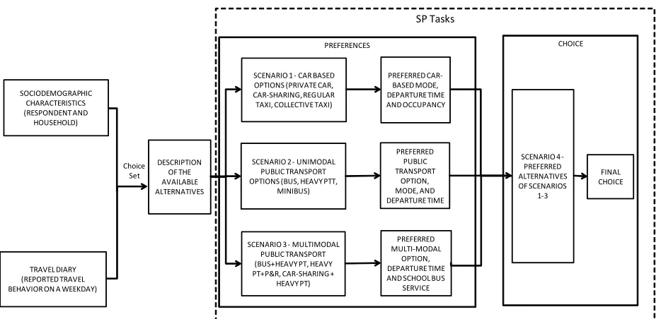
The SP survey organization is schematically shown in Figure 1. In the first section the socio-demographic characteristics of the respondent and his/her household where collected. These included household size and composition, car ownership, identification of the members with driver license and the need to drive children to school.
7
Figure 1: Organization of the survey
The choice set was constructed based on the following:
Socio-demographic characteristics For example car ownership and possession of a driver s license dictated availability of solo driving, possession of a driver s license dictated
availability of one-way car rental, presence of school going children (in a commute trip) dictated the availability of the novel park and ride option, etc.
Origin-destinations: For example, several public transport alternatives were only available in some areas of the LMA, congestion pricing was applicable only to trips involving the central Lisbon, etc.
Trip purpose and departure time: For example, some modal and scheduling alternatives are available only for commuting (e.g. express minibus) and others are not (e.g. if the
respondent had mentioned that there is no flexibility associated with the trip, the departure time choice was not presented).
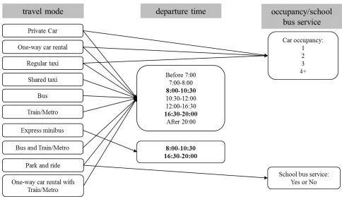
The full multidimensional choice set in the main survey is presented in Figure 21. Except for the
express minibus, none of the alternative modes had time restrictions. Occupancy choice was associated with car based alternatives (with cost implications). The choice of school bus service was associated with train/metro with park and ride. As a result, multidimensional choice set comprised of 135 alternatives in total (Figure 2).
1 This Figure corresponds to the choice set of a person who has availability of all modes and has a school going
children associated with the trip.
PREFERENCES SOCIODEMOGRAPHIC CHARACTERISTICS (RESPONDENT AND HOUSEHOLD) TRAVEL DIARY (REPORTED TRAVEL BEHAVIOR ON A WEEKDAY)
FINAL CHOICE
SCENARIO 3 - MULTIMODAL PUBLIC TRANSPORT (BUS+HEAVY PT, HEAVY PT+P&R, CAR-SHARING +
HEAVY PT) SCENARIO 2 - UNIMODAL
PUBLIC TRANSPORT OPTIONS (BUS, HEAVY PTT,
MINIBUS) SCENARIO 1 - CAR BASED OPTIONS (PRIVATE CAR, CAR-SHARING, REGULAR TAXI, COLLECTIVE TAXI)
PREFERRED CAR-BASED MODE, DEPARTURE TIME AND OCCUPANCY PREFERRED PUBLIC TRANSPORT OPTION, MODE, AND DEPARTURE TIME PREFERRED MULTI-MODAL OPTION, DEPARTURE TIME AND SCHOOL BUS
SERVICE DESCRIPTION
OF THE AVAILABLE ALTERNATIVES
8
Figure 2 Multidimensional choice set
In the SP section, the alternatives were presented sequentially as mentioned in Section 2.3. In the first stage, the respondents were asked to select their preferred alternative in each of the following sub-sets of alternatives (subject to the choice set constraints):
Car group: private car, one-way car rental, regular taxi, shared taxi Public transportation group: bus, light/ metro rail, express minibus
Multimodal group: bus and train/metro, park and ride, one-way car rental with train/metro
The options were introduced using textual descriptions supplemented by images both in the online version and the supplementary computer aided personal interviews. The novelties of the new modes were emphasized in the survey - both in the introductory text for the recruitment and the description of the alternatives.
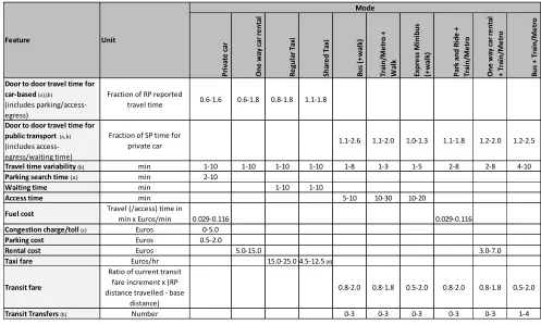
It may be noted that in order to keep the response burden and choice task within a feasible limit, the number of mode specific attributes have been kept to the minimum. The findings of the focus group discussions have been crucial in making this elimination.
9
Table 1: Attribute values and the ranges
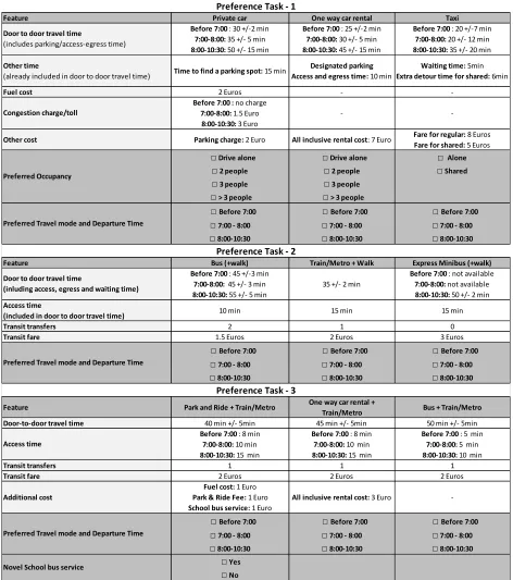
The respondent stated the preferred alternatives in each of the subsets. These preferred subsets were then presented and the respondent was asked to state the final choice (i.e. most preferred alternative out of the three preferred alternatives). For instance, if a respondent with limited flexibility of departure time, owns a car, has a driver's license and has a school going children associated with a commute trip between origin-destinations served by all public transports and involving central Lisbon (and hence congestion charge), he/she can choose from all modes and has three options for departure time choice. An example of the corresponding preference tasks are presented in Figure 3a.
P ri v a te c a r O n e w a y c a r re n ta l R e g u la r T a x i S h a re d T a x i B u s (+ w a lk ) T ra in /M e tr o + W a lk E x p re ss M in ib u s (+ w a lk ) P a rk a n d R id e + T ra in /M e tr o O n e w a y c a r re n ta l + T ra in /M e tr o B u s + T ra in /M e tr o
Door to door travel time for car-based (a),(b)
(includes parking/access-egress)
Fraction of RP reported
travel time 0.6-1.6 0.6-1.8 0.8-1.8 1.1-1.8
Door to door travel time for public transport (a,b)
(includes access-egress/waiting time)
Fraction of SP time for
private car 1.1-2.6 1.1-2.0 1.0-1.3 1.1-1.8 1.2-2.0 1.2-2.5
Travel time variability (b) min 1-10 1-10 1-10 1-10 1-8 1-3 1-5 2-8 2-8 4-10
Parking search time (a ) min 2-10
Waiting time min 1-10 1-10
Access time min 5-10 10-30 10-20
Fuel cost Travel (/access) time in
min x Euros/min 0.029-0.116 0.029-0.116
Congestion charge/toll (c) Euros 0-5.0
Parking cost Euros 0.5-2.0
Rental cost Euros 5.0-15.0 3.0-7.0
Taxi fare Euros/hr 15.0-25.0 4.5-12.5 (d)
Transit fare
Ratio of current transit fare increment x (RP distance travelled - base
distance)
0.8-2.0 0.8-1.8 0.5-2.0 0.8-2.0 0.8-1.8 0.5-2.0
Transit Transfers (b) Number 0-3 0-3 0-3 0-3 0-3 1-4
Mode
Feature Unit
(c) Always 0 for trips not involving Central Lisbon
(d) It may be noted that the travel times for the shared taxi is higher than the travel times of regular taxis (a) The values differed depending on if the destination involved central Lisbon
(b) The values differed depending on RP travel time (i.e. the RP travel times were in bands of <15min, 15-30min, 30-45min
10
Figure 3a: Preference Tasks
Feature Private car One way car rental Taxi Before 7:00 : 30 +/-2 min Before 7:00 : 25 +/-2 min Before 7:00 : 20 +/-7 min
7:00-8:00: 35 +/- 5 min 7:00-8:00: 30 +/- 5 min 7:00-8:00: 20 +/- 12 min
8:00-10:30: 50 +/- 15 min 8:00-10:30: 45 +/- 15 min 8:00-10:30: 35 +/- 20 min
Other time
(already included in door to door travel time) Time to find a parking spot: 15 min
Designated parking Access and egress time: 10 min
Waiting time: 5min
Extra detour time for shared: 6min
Fuel cost 2 Euros -
-Before 7:00 : no charge
7:00-8:00: 1.5 Euro -
-8:00-10:30: 3 Euro
Other cost Parking charge: 2 Euro All inclusive rental cost: 7 Euro Fare for regular: 8 Euros
Fare for shared: 5 Euros
Drive alone Drive alone Alone 2 people 2 people Shared 3 people 3 people
> 3 people > 3 people
Before 7:00 Before 7:00 Before 7:00 7:00 - 8:00 7:00 - 8:00 7:00 - 8:00 8:00-10:30 8:00-10:30 8:00-10:30 Feature Bus (+walk) Train/Metro + Walk Express Minibus (+walk)
Before 7:00 : 45 +/-3 min Before 7:00 : not available
7:00-8:00: 45 +/- 3 min 35 +/- 2 min 7:00-8:00: not available
8:00-10:30: 55 +/- 5 min 8:00-10:30: 50 +/- 2 min
Access time
(included in door to door travel time) 10 min 15 min 15 min
Transit transfers 2 1 0
Transit fare 1.5 Euros 2 Euros 3 Euros
Before 7:00 Before 7:00 Before 7:00 7:00 - 8:00 7:00 - 8:00 7:00 - 8:00 8:00-10:30 8:00-10:30 8:00-10:30
Feature Park and Ride + Train/Metro One way car rental +
Train/Metro Bus + Train/Metro Door-to-door travel time 40 min +/- 5min 45 min +/- 5min 50 min +/- 5min
Before 7:00 : 8 min Before 7:00 : 8 min Before 7:00 : 5 min
7:00-8:00: 10 min 7:00-8:00: 10 min 7:00-8:00: 5 min
8:00-10:30: 15 min 8:00-10:30: 15 min 8:00-10:30: 10 min
Transit transfers 1 1 1
Transit fare 2 Euros 2 Euros 2 Euros
Additional cost
Fuel cost: 1 Euro
Park & Ride Fee: 1 Euro
School bus service: 1 Euro
All inclusive rental cost: 3 Euro
Before 7:00 Before 7:00 Before 7:00 7:00 - 8:00 7:00 - 8:00 7:00 - 8:00 8:00-10:30 8:00-10:30 8:00-10:30
Yes No
Preference Task - 1
Preference Task - 2
Preference Task - 3
Preferred Travel mode and Departure Time
Novel School bus service
Preferred Travel mode and Departure Time Access time
Door to door travel time
(includes parking/access-egress time)
Congestion charge/toll
Preferred Occupancy
Preferred Travel mode and Departure Time
11
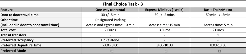
Figure 3b: Final Choice Task
Assuming that the preferred modes in these are One way car rental, Express minibus and Bus with Train/Metro along with his preferred departure times and occupancy, the final choice task is shown in Figure 3b.
In each SP exercise, each respondent was presented with three scenarios (each containing up to three preferences) followed by a choice scenario (with three alternatives). Two SP exercises were provided to each respondent ultimately yielding up to twelve responses per individual.
It may be noted that in the pilot stage, the full effect of departure time on levels of attributes was not presented up front. That is, the respondents were shown alternatives corresponding to their current departure time given the option to revise the departure time. Revision of the departure time led to a new set of attribute values. This was reported to be confusing by the respondents and led to non-intuitive coefficients of cost for the congestion charging scenarios (54). This led to the revised design where the attributes associated with each departure time were presented up front and the respondent could simultaneously select the mode and the departure time. This made the SP scenarios more realistic and robust. In terms of the survey length and the ease of understanding the details of the smart modes, the respondents responded positively.
It may be noted that the availability and levels-of-service of the modes presented in the first choice dimension varied substantially with time-of-day. For instance, travelling by non-shared modes during peak hours involved payment of variable rates of the congestion charge, travel times and frequency of public transport modes differed depending on the time of day, etc. Hence, a large number of rules are set to generate attribute levels. Furthermore, the inter-relationships among different modes are considered, e.g. the cost of transit pass is kept the same across all modes for a specific individual scenario.
3.2. Data
The survey was administered to the residents of the Lisbon Metropolitan Area (LMA) over the internet (1,384 SP observations from 754 respondents) in May-June 2009 and supplemented by computer aided personal interviews (988 SP observations from 494 respondents) during
September 2009. Statistical analysis reveals that the sample has significant heterogeneity of socio-economic characteristics.
The age of the respondents ranges evenly from 18 to 65 or more. There are appropriate portions for respondents in each working status, such as full-time employees, part-time employees, students, worker-students, unemployed people, and retired people. In terms of household characteristics, the income ranged from less than 1000 Euros/month to more than 5000 Euros/month; around 41 % of
Feature One way car rental Express Minibus (+walk) Bus + Train/Metro Door to door travel time 30 +/- 5 min 50 +/- 2 mins 50 min +/- 5min
Other time (included in door to door travel time)
Designated Parking
Access and egress time: 10 min Access time: 15 min Access time: 5 min
Total cost 7 Euros 3 Euros 2 Euros
Transit transfers - - 1
Preferred Occupancy Drive alone -
-Preferred Departure Time 7:00 - 8:00 8:00-10:30 8:00-10:30
Preferred Mode
12 the respondents have one car in the household, and 47% have two cars or more. Overall, although the data is not a fully representative sample; it has a good coverage of the demographics of the population of the LMA.
The data regarding commute trips (commuting to work or school, and commuting with intermediate stops) and non-commute trips are analysed separately because of the potential differences in flexibility levels (particularly for departure time) and time and cost sensitivities among these trips.
Most commute trips (69%) are concentrated during the morning peak period, between 8:00 and 10:30, with an additional 17% of trips departing between 7:00 and 8:00. The average commute duration is around 40 minutes, consistent with the size and land use of the LMA. For 27% of the trips, travel times range between of 15 to 30 minutes, 42% between 30 to 60 minutes, and 18% between 60 to 90 minutes. 38.6 % of the trips enter the central area of Lisbon, aimed to be subjected to a congestion charge from 7:00 to 20:00. About 36% of the respondents own a transit pass. Among car users, significant proportions (62%) currently do not share their car trip with anyone else.The aggregate travel behaviour collected in the survey is presented in Table 2.
Table2: Aggregate travel behavior
Mean
Standard Deviation
Number of trips by individual 2.69 1.17
Number of public transport trips 0.87 1.18
Number of car trips 1.79 1.57
Number of non-motorized trips 0.03 0.19
Modal split
Public transport 32.5%
Car 66.5%
Non-motorized 1.0%
Occupancy
Drive alone 53.8%
2 people 32.2%
3 people 7.8%
>3 people 6.2%
4. Model Development
The estimated multidimensional discrete choice model is based on the Random Utility
13 available options and selects the one with the highest utility. The systematic part of the utility ( ) is influenced by attributes of the modes (which varied with departure time and occupancy) and the characteristics of the decision maker.
The design setting and the choice complexity in this context, however, raised a number of
methodological issues. In particular, the large choice set and the multidimensional choice structure is expected to result in complex correlations among the alternatives. The non-traditional survey design (i.e. sequential choice set presentation) also adds complexity to the model structure.
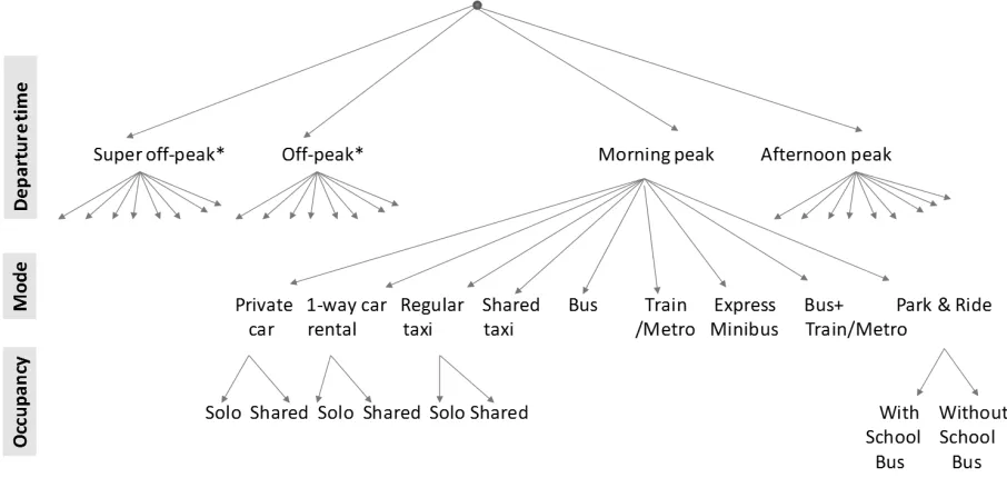
[image:14.612.72.525.283.498.2]Based on expected correlation structures, different Nested Logit (NL) model specifications were tested. These included nesting departure times within modes, nesting modes within the presented departure time windows, nesting modes within aggregated departure times, nesting based on the mode groupings adopted in the survey, etc. Among these, the model presented in Figure 4 is found to be the best one in terms of goodness-of-fit.
Figure 4: Structure of the selected model
(* Express minibus is not presented as an option in these time periods)
Simple NL models, however, ignore the correlations among multiple observations of the same respondent (panel effect). Further, there may be scale differences between the two sets of SP tasks (preferences and the choices). In order to capture the intra-respondent correlation within the nested framework, a Nest specific error component model with panel formulation has been used. These nest specific error components are assumed to vary across the population but remain constant over multiple observations of the same individual. Given the selected nesting structure, four nest specific error components are included in the mixed logit models for the four subsets of
14 scale difference between the two types of stated responses (preferences and choices), separate individual specific error components that vary between the preferences and the final choice have been added.
The final model formulation can be expressed as the following:
Where,
: the utility of alternative (unique combination of mode, departure time and occupancy) of observation of respondent
: observed independent variables of alternative of observation from respondent that do not involve unobserved taste heterogeneity
: fixed coefficients for observed independent variables that do not involve unobserved taste heterogeneity
: observed independent variables of alternative of observation of respondent which involve unobserved taste heterogeneity (such as inertia to RP choice, etc.)
: mean value of the random coefficient corresponding to
: random part of the coefficient for the attribute with unobserved taste heterogeneity forrespondent n for stated preferences data,
: random part of the coefficient for the attribute with unobserved taste heterogeneity for respondent n for stated choice data,
: equals 1 if is a stated preferences observation, 0 otherwise,
: equals 1 if is a stated choices observation, 0 otherwise,
: nest specific error component for respondent n associated with morning peak period (N1 nest),
: nest specific error component for respondent n associated with afternoon peak period (N2 nest),
: nest specific error component for respondent n associated with super off-peak period (start/end of the day, N3 nest),
: nest specific error component for respondent n associated with off-peak period (N4 nest),
: equals 1 if alternative belongs to alternatives associated with morning peak period (N1 nest), 0 otherwise,
: equals 1 if alternative belongs to alternatives associated with afternoon peak period (N2 nest), 0 otherwise,
15 : equals 1 if alternative belongs to alternatives associated with off-peak periods (N4 nest), 0 otherwise,
: random error term which follows identical and independent extreme value distribution.
The choice probabilities of alternatives are obtained by integrating conditional choice probabilities over the specified distributions of nest specific ( and response type specific
error components ( .
Where,
: available alternative for observation and respondent ,
the unconditional choice probability of alternative for observation and respondent ,
: conditional choice probability of alternative for observation and respondent .
Given the high dimensionality of integration, simulated maximum likelihood estimation has been used to estimate the model coefficients. In simulated maximum likelihood estimation, the true probabilities are replaced with the simulated probabilities using random/quasi random draws and used for calculating the simulated log-likelihood (SLL) and the set of parameters that maximizes SLL has been derived. In this case, Halton Sequence has been applied to draw quasi-random realizations from the underlying error process (55) during the estimation. Given the model complexity, the software package FastBiogeme (56) which enables parallel computing has been used. The number of Halton Draws used in this case was 1000.
It may be noted that the panel specification of the error components were satisfied the order and rank conditions (57), normalization was not required.
5. Estimation Results
Separate models were estimated for commute and non-commute trips since the flexibilities in departure time and occupancies are expected to be different in the two scenarios. This was confirmed by the estimation results where the parameter estimates were found to be significantly different between the two cases.
16 correct sign and statistical significance of the model parameters have been used as the basis of the model selection2.
The estimation results of the best models are presented in Table 3.
2 In some cases, statistically non-significant parameters with intuitive signs have been retained for comparison
purposes. Given the commute and non-commute trips were estimated with different datasets, their adjusted
rho-squared values cannot be cross-compared. However, in both cases, the final model had better rho-rho-squared values than
17
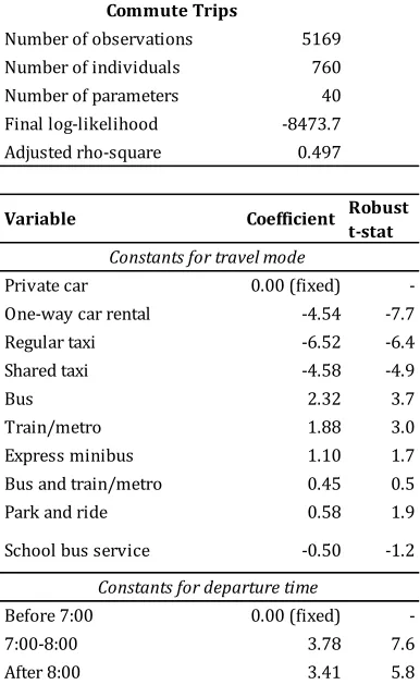
Table 3: Estimation results
Number of observations 5169 Number of observations 3624
Number of individuals 760 Number of individuals 488
Number of parameters 40 Number of parameters 34
Final log-likelihood -8473.7 Final log-likelihood -5222.9
Adjusted rho-square 0.497 Adjusted rho-square 0.587
Variable Coefficient Robust
t-stat Variable Coefficient
Robust t-stat
Private car 0.00 (fixed) - Private car 0.00 (fixed) -
One-way car rental -4.54 -7.7 One-way car rental -0.81 -10.1
Regular taxi -6.52 -6.4 Regular taxi -1.08 -7.3
Shared taxi -4.58 -4.9 Shared taxi -0.50 -5.4
Bus 2.32 3.7 Bus -0.91 -6.4
Train/metro 1.88 3.0 Train/metro -1.04 -4.8
Express minibus 1.10 1.7 Express minibus -2.48 -2.6
Bus and train/metro 0.45 0.5 Bus and train/metro -0.04 -0.3
Park and ride 0.58 1.9 Park and ride -1.27 -4.6
School bus service -0.50 -1.2
Before 7:00 0.00 (fixed) - Before 7:00 0.00 (fixed) -
7:00-8:00 3.78 7.6 7:00-8:00 4.96 6.0
After 8:00 3.41 5.8 8:00-10:30 4.83 5.7
10:30-12:00 4.74 7.1
12:00-16:30 2.74 3.9
16:30-20:00 0.62 2.2
After 20:00 2.78 1.8
1 people 0.00 (fixed) - 1 people 0.00 (fixed) -
2 people -0.26 -2.5 2 people -0.69 -4.0
3 people, 4 people or more -0.95 -9.1 3 people, 4 people or more -1.68 -8.4
Car-based group -0.21 -2.3 Car-based group -0.33 -2.2
Public transport group -0.93 -7.2 -0.39 -2.4
Multimodal group -0.66 -4.6
Car-based group -0.21 -2.5 Car-based group -0.18 -1.9
Public transport group -0.67 -2.4 -0.16 -1.6
Multimodal group -0.30 -2.6
Standard deviation of the random coefficient for the natural logarithm of travel time for preference data
2.12 7.5
Standard deviation of the random coefficient for the natural logarithm of travel time for choice data
0.27 0.7
Public transport and multimodal groups
Public transport and multimodal groups
Natural logarithm of total time (Minute)
Non-commute Trips
Constants for travel mode
Constants for departure time
Constants for occupancy
Natural logarithm of total cost (Euro)
Commute Trips
Natural logarithm of total time (Minute) Natural logarithm of total cost (Euro)
Constants for travel mode
Constants for departure time
18
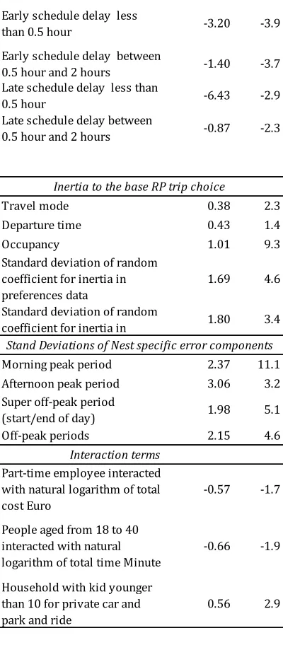
Table 3: Estimation results (contd.)
5.1 Commute Trips
In the cleaned sample, there were 5169 SP observations from 760 respondents with trip purposes of commuting to work, commuting to school, or commuting with intermediate stops. The utility
Variable Coefficient Robust
t-stat Variable Coefficient
Robust t-stat
Number of transfers -0.10 -2.0 Number of transfers -0.19 -1.7
Size of departure time
intervals 1.00 (fixed) Size of departure time intervals 1.00 (fixed)
Early schedule delay less
than 0.5 hour -3.20 -3.9
Early schedule delay less than
0.5 hour -3.12 -5.4
Early schedule delay between
0.5 hour and 2 hours -1.40 -3.7
Early schedule delay between
0.5 hour and 2 hours -1.28 -1.9
Late schedule delay less than
0.5 hour -6.43 -2.9
Late schedule delay less than
2 hours -0.95 -2.0
Late schedule delay between
0.5 hour and 2 hours -0.87 -2.3
Late schedule delay between 2
hours and 5 hours -1.60 -2.4
Late schedule delay between 5
hours and 10 hours -0.09 -1.2
Travel mode 0.38 2.3 Travel mode 1.19 7.9
Departure time 0.43 1.4 Departure time 1.37 1.4
Occupancy 1.01 9.3 Occupancy 2.29 12.3
Standard deviation of random coefficient for inertia in preferences data
1.69 4.6
Standard deviation of random
coefficient for inertia in 1.80 3.4
Morning peak period 2.37 11.1 Morning peak period 5.83 8.8
Afternoon peak period 3.06 3.2 Afternoon peak period 5.63 7.6
Super off-peak period
(start/end of day) 1.98 5.1
Super off-peak period
(start/end of day) 3.87 4.7
Off-peak periods 2.15 4.6 Off-peak periods 5.18 6.6
Part-time employee interacted with natural logarithm of total cost Euro
-0.57 -1.7 People aged between 18 and 40
for smart travel options 1.39 5.0
People aged from 18 to 40 interacted with natural logarithm of total time Minute
-0.66 -1.9
Household with kid younger than 10 for private car and park and ride
0.56 2.9 Inertia to the base RP trip choice
Stand Deviations of Nest specific error components
Interaction terms
Stand Deviations of Nest specific error components Inertia to the base RP trip choice
Commute Trips Non-commute Trips
Other attributes
Piecewise linear function for schedule delay (Hour) Piecewise linear function for schedule delay (Hour)
Other attributes
19 function includes alternative specific constants, attributes of the smart modes and services (and their interaction terms with socio-economic variables), attributes specific for departure time, inertia to RP trip choices, and the error components (nest-specific and response type specific).
Globally, signs and coefficient sizes are consistent with prior beliefs. Alternative specific constants are considered separately for travel mode, departure time, occupancy, and school bus service. All else being equal, traditional public transport modes are found to be popular for commute trips. This is probably due to the good service of the existing public transport in Lisbon and the inconvenience of using the car during traffic congestion periods. All else being equal, one-way car rental and shared taxi are found to be preferred to regular taxi but substantially less preferred than private cars or public transport options.
In terms of departure time, all else being equal, 7:00-8:00 is the preferred slot and before 7:00 is the least preferred.
In terms of occupancy, all else being equal, solo travel is found to be the most preferable and sharing the car with more than 3 people is found to be the least preferable. Consistent with the focus group results, the novel park and ride system with the school bus service is not favoured.
The main attributes of the alternatives are travel time and cost. Here, travel time is the door-to-door time, including access and egress time, in-vehicle time, parking search time, waiting time; travel cost includes fuel cost, rental cost, congestion charge, parking costs and fare (Table 1). It may be noted that the sensitivity to the different components of the time and cost coefficients (e.g. separate coefficients of access time, parking search time, etc. and fuel cost, congestion charge, rental cost, etc.) have been tested but the differences were found to be statistically insignificant (and often non-intuitive). This emphasizes that travellers are more sensitive to the door-to-door travel times as opposed to the components.
In terms of functional forms, the linear specifications did not provide acceptable values and logarithmic values of travel time and costs are used in the utility functions. This indicates that people s sensitivities to the unit change in travel time or cost are likely to decrease when they are facing longer travel time or higher travel cost. As expected, the coefficients for the logarithmic values of these two attributes are negative. Sensitivities to travel time and cost are found to vary with travel modes. People appear to be less sensitive to the travel cost of the car-based group (private car, one-way car rental, regular taxi, and shared taxi) and most sensitive to the travel cost of public transport group. Further, random coefficients of travel times and costs have been tested and estimation results indicate significant inter-respondent heterogeneity in the coefficient of the logarithm of travel time (but insignificant for travel cost). The standard deviation of this random term (which also captures the panel effect) has been found to differ significantly between the stated choice and preference data.
In addition, the systematic effect of the socio-demographic segmentation has been tested according to a priori hypotheses. According to the estimation results, respondents aged from 18 to 40 have greater sensitivity to travel time perhaps because they are more time constrained. Part-time
employees are found to be slightly more sensitive to travel cost As a result people s WTP for saving travel time is found to vary with travel modes and market segments (as detailed in the next
20 sensitivity to travel time variability (for the car-based group) is found to be statistically
insignificant.
In the SP survey, departure time is divided into seven intervals with unequal lengths. Usually, events are more likely to occur during longer time intervals. In order to capture this phenomenon, the natural logarithm of the interval length is included in the utility functions and the
corresponding coefficient is constrained to one (see 58 for details).
Schedule delay is a fundamental concept in modelling departure time choice. It accounts for the disutility caused by traveling at times other than the desired departure time. Departure time of the base surveyed RP trip is assumed to be the desired one and the schedule delay is calculated based on that. Since people are likely to minimize early/late schedule delay when rescheduling, they are more likely to select the departure time interval closest to the departure time of the base RP trip and sensitivities to the unit change of schedule delay are likely to decrease with the increasing value of schedule delay. Therefore, piecewise linear functions of schedule delay have been used to capture the sensitivity to the schedule delay. As expected, the coefficients for piecewise linear functions of early schedule delay and late schedule delay are negative, because increasing schedule delay may increase the disutility of departure time interval. In general, respondents are more sensitive to late schedule delay than early schedule delay for commute trips. The disutility of early/late schedule delay increases when early/late schedule delay is less than 2 hours, and remains a negative constant value when early/late schedule delay is longer than 2 hours. This can be explained by people s strong aversion to making large schedule adjustments (longer than 2 hours) for commute trips. There is no big difference for them when schedule delay is longer than 2 hours.
In the SP survey, respondents are likely to make the decisions in the context of their base RP trips. Therefore, their preferences and choices may be affected by their RP choices. As expected, the inertia coefficients are found to be positive and significant. Respondents have very strong inertia to select the same occupancy as in the base RP trips because trip sharing is mainly with family
members according to the focus group discussion. The inertia to RP departure time is slightly stronger than the inertia to RP travel mode, probably due to the constraints of work and school hours. Estimation results also indicate significant inter-respondent heterogeneity in the inertia coefficient for travel mode (but not for departure time and occupancy). The standard deviation of this random term has been found to differ significantly between the stated choice and preference data.
21 The model specification does not include the ratio of travel cost and income, which is commonly seen in travel mode choice models. This is due to the poor performance and worse goodness-of-fit of models including this ratio which may be due to the fact that more than 20% of the respondents refuse to provide the ranges of their household income in the SP survey and some respondents may have reported their household income incorrectly. The effect of trip length has also been found to be insignificant, potentially due to the high correlation with the travel time and cost.
5.2 Non-commute Trips
In the cleaned sample, there are 3624 SP observations from 488 respondents with non-commute trip purposes, such as shopping, leisure/entertainment, picking up/dropping off/accompanying someone, etc.
The results have both similarities and dissimilarities with the commute trip model results. The utility functions include alternative specific constants, main attributes for levels of service, attributes specific to departure time, inertia to RP trip choices and the nest specific error
components (with panel effect) as in the commute model, but the inter-respondent heterogeneity have been found to be insignificant for all potential variables.
Considering the alternative specific constants, all else being equal, a private car is the most preferred alternative, followed by multimodal alternatives, shared taxi, one-way car rental, bus, regular taxi, train/metro, park and ride and express minibus. It may be noted that compared to the commute trips, shared taxi and one-way car rental are more favoured and express minibus is less preferred for non-commute trips.
Non-commute trips typically have higher flexibility in terms of the departure time. Consequently, the alternative specific constants for the departure time reflect a wider variation compared to the commute trips. Though it was originally hypothesized that non-commute trips will exhibit more flexibility in terms of occupancy, the estimated coefficients reveal a high disutility for sharing the trips with others. This may be because formal carpool is easier to arrange for commute trips given their regularity and frequency.
Respondents are found to be less sensitive to the travel time of non-commute trips compared to commute trips, possibly because there are less time constraints for non-commute trips. The sensitivity to cost, on the other hand, is more varied: the cost sensitivity being higher compared to commute trips for car-based trips but lower for corresponding public transport trips. It may be noted, the inter-respondent heterogeneity in the sensitivities to travel times and costs has been found to be insignificant. Other attributes include a number of transfers for bus and train/metro, whose coefficients are negative as expected.
22 The inertia coefficients, although statistically insignificant for departure time choice, appear to be higher in magnitude for mode and occupancy when compared with the commuting case. This may be due to unobserved constraints associated with these non-commute trips that are captured in the inertia term.
Further, estimation results indicate an additional preference for the smart travel options among respondents aged between 18 and 40. It may be noted the heterogeneity has also been tested using smaller age groups but the differences between the sub groups have not been found to be
statistically different. The effect of being students and working part-time have been tested as a separate covariate by including a student specific dummy but it was not found to be statistically significant.
The random parts of mixed logit model include four nest specific error components for the subsets of alternatives associated with morning peak period, afternoon peak period, start/end of the day, and off-peak periods. These error components vary across the population but are constant for multiple observations from each individual and capture the panel effect. The standard deviations of these nest specific error component are much higher for non-commute trips compared to commute trips indicating higher extent of heterogeneity. Further, the standard deviation is slightly higher in the morning peak than the afternoon peak indicating higher extent of heterogeneity.
6. Willingness-to-pay Analysis and Policy Implications
Introducing the natural logarithms of travel time and cost in the model specifications leads to the
varying values of , which depend on the ratio of two coefficients and the
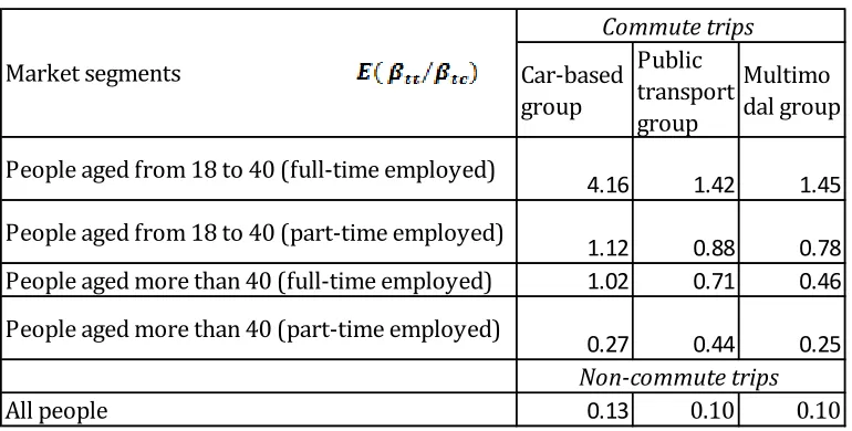
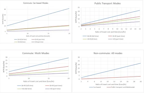
[image:23.612.72.457.504.699.2]actual ratio of travel cost and time . Table 4 presents the expected ratio of two coefficients for different trip purposes, travel modes, and market segments. The approximate WTP values are calculated assuming the range of tc/tt for the car-based group to be 5 to 20 Euros per hour, for the public-transport group to be 2 to 15 Euros per hour, and for the multimodal group to be 5 to 20 Euros. The WTP variations are presented in Figure 5.
Table 4: Ratio of coefficients for travel time (in hour) and cost (in Euros)
Car-based group
Public transport group
Multimo dal group
People aged from 18 to 40 (full-time employed)
4.16 1.42 1.45
People aged from 18 to 40 (part-time employed)
1.12 0.88 0.78
People aged more than 40 (full-time employed) 1.02 0.71 0.46
People aged more than 40 (part-time employed)
0.27 0.44 0.25
All people 0.13 0.10 0.10
Non-commute trips Market segments
23
Figure 5: WTP ranges
As seen in Figure 5, the VOT values for car-based, public transport based and multimodal commute trips range from 2-83 euros/hr, 2-20 euros/hr and 3-30 euros/hr respectively. To the best of our knowledge, there has not been any recent academic study in Portugal that investigates VOT in a similar intra-urban context for direct validation of these values. However, in a previous SP study that investigated VOT in case of inter urban trips VOT of the car and bus users in the context of possible shift to high speed rail have been reported to be euros hour and euros hour respectively 60). The intra-urban VOT derived from the current study, though not directly comparable, are in agreement with the ranges obtained from that inter-urban study.
Another point to note is the strong difference between WTP of full and part time workers. Part time is usually associated with a salary reduction, roughly proportional to the working time reduction. In Portugal, it is also more common in less specialized occupations, which very often are not well paid. However, most importantly, the part-time workers are often the ones with more flexibility in
working hours and hence more likely to change their departure times in response to the proposed changes in levels of service, congestion charge in particular. These factors are expected to have contributed to the substantially lower WTPs of these groups.
The detailed insights and associated policy implications of the findings are listed below.
24 overpay for saving travel time. For commute trips, the expected values of WTP for car-based group are much higher than the expected values of WTP for public transport and multimodal groups. Targeting the commute trips during the planning of the smart modes can thus be financially more profitable. On the other hand, at the system level, if the network is likely to benefit significantly from peak spreading (as is the case of Lisbon), the focus may be well on the non-commute trips where a temporally differential pricing may be particularly effective given the low WTP values.
Secondly, for non-commute trips, market segments do not have significant impacts on the values of WTP, but for the commute trips, respondents in the 18-40 age range who are employed full time have significantly higher WTP for all modes followed by respondents in that age range and
employed part-time. This finding can be used effectively in the planning and marketing of the smart modes to maximize their potential.
Thirdly, the results also reveal that the WTP is more than double for the car-based modes compared to public transport and multimodal alternatives for the 18-40 full-time employed groups. This can be an important factor in cross-evaluation of the car vs. public transport based smart mobility options.
Finally, the WTP values for the public transport and multimodal options have close resemblance in trends in case of the commute trips while for non-commute trips, the WTP values are not
significantly different between these two groups. This is an interesting finding given that while shortlisting the potential smart modes for detailed analysis (9, 10), the multimodal options were expected to be associated with higher WTP compared to public transport (only) options. However, this may have also been a result of the fact that this survey was focused only on mode, departure time and occupancy choice as opposed to an even wider spectrum (e.g. destination choice, activity choice) or mid-term (e.g. car ownership) and long term (e.g. change in residential location) decisions and need to be used with caution.
25 While the WTP measures calculated from the model estimates can be used to better inform
effective pricing strategies for the proposed smart modes and services, these insights can also contribute towards more effective implementation strategies. Examples include focusing on door-to-door travel time reduction as opposed to reduction of a specific component or variability, employing more resources for investigating the barriers for increased formal and informal car sharing and school bus based services and dedicating more resources in overcoming them, etc.
7. Concluding Remarks
In this research, the acceptability and willingness-to-pay for three smart travel options have been tested alongside conventional congestion management and public transport improvement options in the context of the Lisbon Metropolitan Area. The policy implications of the results have been highlighted in the preceding section.
In terms of the methodology, the research extends the state-of-the-art in smart mode choice analysis by proposing and demonstrating a detailed data collection and model development framework for quantifying the preferences for the smart mobility options alongside existing transport options and their variants in a multidimensional choice spectrum. The results demonstrate the level of details that can be obtained from multidimensional surveys and joint modeling of mode-departure time choice occupancy as opposed to focus group surveys or simpler SP surveys. For instance, it shows that inclusion of the departure time and occupancy choice dimensions allows us to get insights about what will be the extent of peak spreading and
formal/informal car sharing and which segments are more flexible and/or price sensitive; while a simpler SP would have ignored the possibilities of departure time and occupancy changes and over stated the share of smart modes and the WTP values. Similarly, the research demonstrates the feasibility of conducting a combined analysis of smart mobility options and variants of existing options. Since investigating the smart modes in isolation has the risk of overestimating the
potential benefits of a particular smart mode or smart modes in general, the research can be useful to replicate in cities which are looking at a combination of different options to influence demand and supply to address the transport problems and interested to conduct a comprehensive
evaluation (as is the case in Lisbon). The research is thus expected to serve as a good example of the robustness of a detailed study - demonstrating the additional insights it can offer compared to a simpler study. It also demonstrates the challenges associated with designing, administering and analyzing complex surveys and addressing the data issues by using appropriate model structures. It may be noted that some aspects of the survey design and model development methodologies have the potential to be transferred beyond the realm of transport research (e.g. marketing, finance, health) where similar challenges arise due to large and/or multidimensional choice sets.
This study has, however, several limitations. Firstly, the findings are based on SP data and though the SP surveys have been designed and pre-tested carefully, the findings can be subjected to
26 SP survey included only mode, departure time and occupancy choice. Extending the choice
spectrum even further to include route, destination, and activity choices is likely to provide more robust results.
Acknowledgement
This research was made possible by the generous support of the Government of Portugal through the Portuguese Science Foundation (FCT_- Fundação para a Ciência e a Tecnologia) and was undertaken as part of the SCUSSE (Smart Combination of passenger transport modes and services in Urban areas for maximum System Sustainability and Efficiency) initiative of the MIT-Portugal Program.
References
1. Dudley, G. (2013). Why do ideas succeed and fail over time? The role of narratives in policy windows and the case of the London congestion charge. Journal of European Public Policy, (ahead-of-print), 1-18.
2. Prud'homme, R., Koning, M., Lenormand, L., & Fehr, A. (2012). Public transport congestion costs: The case of the Paris subway. Transport Policy, 21, 101-109.
3. Carpintero, S., & Gomez-Ibañez, J. A. (2011). Mexico's private toll road program reconsidered. Transport Policy, 18(6), 848-855.
4. May, A. D., and C. A Nash. (1996) Urban Congestion: A European Perspective on Theory and Practice. Annual Review of Energy and the Environment, No. 21, 1996, pp. 239-260.
5. Correia, G. H. D. A., & Viegas, J. M. (2008). Structured Simulation-Based Methodology for Carpooling Viability Assessment. In Transportation Research Board 87th Annual Meeting (No. 08-0199).
6. Litman, T. (2011). London congestion pricing: Implications for other cities. Victoria Transport Policy Institute. 7. Barnes, I. C., Frick, K. T., Deakin, E., & Skabardonis, A. (2012). Impact of Peak and Off-Peak Tolls on Traffic in San
Francisco-Oakland Bay Bridge Corridor in California. Transportation Research Record: Journal of the Transportation Research Board, 2297(1), 73-79.
8. Dudley, G. (2013). Why do ideas succeed and fail over time? The role of narratives in policy windows and the case of the London congestion charge. Journal of European Public Policy, (ahead-of-print), 1-18.
9. Viegas J M de Abreu e Silva J and Arriaga R )nnovation in Travel modes and Services in Urban Areas and their Potential to Fight Congestion Presented at the st Annual Planning Conference on Planning Research Evaluation in Planning, Porto, Portugal, May 30th.
10. Mitchell, J., Chin R. and Sevtsuk A. (2008) The Media Laboratory City Car: A New Approach to Sustainable Urban Mobility, Massachusetts Institute of Technology, Cambridge, MA.
11. Chorus, C.G., Molin, E.J. and Van Wee, B., 2006. Travel information as an instrument to change car drivers travel choices: a literature review. EJTIR, 6 (4), 2006.
12. Buliung, R., Soltys, K., Habel, C. and Lanyon, R., 2009. Driving factors behind successful carpool formation and use. Transportation Research Record: Journal of the Transportation Research Board, (2118), pp.31-38. 13. Correia, G. and Viegas, J.M., 2011. Carpooling and carpool clubs: Clarifying concepts and assessing value
enhancement possibilities through a Stated Preference web survey in Lisbon, Portugal. Transportation Research Part A: Policy and Practice, 45(2), pp.81-90.
14. Atasoy, B., Ikeda, T., Song, X. and Ben-Akiva, M.E., 2015. The concept and impact analysis of a flexible mobility on demand system. Transportation Research Part C: Emerging Technologies, 56, pp.373-392.
15. Shin, J., Bhat, C.R., You, D., Garikapati, V.M. and Pendyala, R.M., 2015. Consumer preferences and willingness to pay for advanced vehicle technology options and fuel types. Transportation Research Part C: Emerging Technologies, 60, pp.511-524.
16. Blau M A Driverless Vehicles Potential )nfluence on Cyclist and Pedestrian Facility Preferences, Doctoral dissertation, The Ohio State University.
27
18. Khattak, A., Polydoropoulou, A. and Ben-Akiva, M., 1996. Modeling revealed and stated pretrip travel response to advanced traveler information systems. Transportation Research Record: Journal of the Transportation
Research Board, (1537), pp.46-54.
19. Vrtic, M., Schüssler, N., Erath, A. and Axhausen, K.W., 2007. Route, mode and departure time choice behaviour in the presence of mobility pricing. ETH, Eidgenössische Technische Hochschule Zürich, IVT, Institut für
Verkehrsplanung und Transportsysteme.
20. Choudhury, C.F., Yang, L., Ben-Akiva, M. and Abreu, J., 2009. Dealing with large number of travel modes in stated preference surveys. In 12th International Conference on Travel Behavior Research, Jaipur, India.
21. Schaefers, T., 2013. Exploring carsharing usage motives: A hierarchical means-end chain analysis. Transportation Research Part A: Policy and Practice, 47, pp.69-77.
22. Sun, Z., Arentze, T. and Timmermans, H., 2012. A heterogeneous latent class model of activity rescheduling, route choice and information acquisition decisions under multiple uncertain events. Transportation research part C: emerging technologies, 25, pp.46-60.
23. Zheng, J., Scott, M., Rodriguez, M., Sierzchula, D., Guo, J. and Adams, T. (2009). Carsharing in a University
Community Assessing Potential Demand and Distinct Market Characteristics, Transportation Research Record: Journal of the Transportation Research Board, 2110, 18-26.
24. Ben-Elia, E. and Shiftan, Y., 2010. Which road do I take? A learning-based model of route-choice behavior with real-time information. Transportation Research Part A: Policy and Practice, 44(4), pp.249-264.
25. Chorus, C.G., Walker, J.L. and Ben-Akiva, M., 2013. A joint model of travel information acquisition and response to received messages. Transportation Research Part C: Emerging Technologies, 26, pp.61-77.
26. Efthymiou, D. and Antoniou, C., 2016. Modeling the propensity to join carsharing using hybrid choice models and mixed survey data. Transport Policy, 51, pp.143-149.
27. Bolduc, D., Boucher, N., Alvarez-Daziano, R. (2008) Hybrid choice modeling of new technologies for car choice in Canada, Transportation Research Record: Journal of the Transportation Research (1981), pp. 63 71.
28. Davidson JD (1973) Forecasting traffic on STOL.Operations Research Quarterly 24: 561 9.
29. Louviere JJ, Meyer R, Stetzer F & Beavers LL (1973) Theory, methodology and findings in mode choice behaviour. Working Paper No. 11, The Institute of Urban and Regional Research, The University of Iowa, Iowa City.
30. Hensher, D. A. (1994). Stated preference analysis of travel choices: the state of practice. Transportation, 21(2), 107-133.
31. Louviere, J. J., Hensher, D. A., & Swait, J. D. (2000). Stated choice methods: analysis and applications. Cambridge University Press.
32. Li, Z., & Hensher, D. A. (2012). Congestion charging and car use: A review of stated preference and opinion studies and market monitoring evidence. Transport Policy, 20, 47-61.
33. Swait, J., & Adamowicz, W. (1996). The effect of choice environment and task demands on consumer behavior: discriminating between contribution and confusion. Department of Rural Economy, Faculty of Agriculture & Forestry, and Home Economics, University of Alberta.
34. Rose J. and Hensher D. (2006) Handling individual specific availability of alternatives in stated choice experiments' in Travel Survey Methods: Quality and Future Directions, ed. P Stopher and C Stecher, Elsevier, Oxford, UK pp. 347-71.
35. Rose, J. M., Bliemer, M. C., Hensher, D. A., & Collins, A. T. (2008). Designing efficient stated choice experiments in the presence of reference alternatives. Transportation Research Part B: Methodological, 42(4), 395-406. 36. Bliemer, M. C., Rose, J. M., & Hensher, D. A. (2009). Efficient stated choice experiments for estimating nested logit
models. Transportation Research Part B: Methodological, 43(1), 19-35.
37. Adamowicz W., Louviere J., Williams M. (1994) Combining stated and revealed reference methods for valuing environmental amenities, Journal of Environmental Economics and Management, 26, 271 292.
38. Brazell, J. D., & Louviere, J. J. (1998). Length effects in conjoint choice experiments and surveys: an explanation based on cumulative cognitive burden. Department of Marketing, The University of Sydney, July.
39. Dellaert B.G.C., Brazell J. D. and Louviere J. (1999) The effect of attribute variation on consumer choice consistency, Marketing Letters, 10 (2), 139 148.