Robust Mixed-Criticality Systems

White Rose Research Online URL for this paper:

http://eprints.whiterose.ac.uk/130366/

Version: Accepted Version

Article:

Burns, Alan orcid.org/0000-0001-5621-8816, Davis, Robert Ian

orcid.org/0000-0002-5772-0928, Baruah, Sanjoy et al. (1 more author) (2018) Robust

Mixed-Criticality Systems. IEEE Transactions on Computers. pp. 1478-1491. ISSN

0018-9340

https://doi.org/10.1109/TC.2018.2831227

eprints@whiterose.ac.uk https://eprints.whiterose.ac.uk/ Reuse

Items deposited in White Rose Research Online are protected by copyright, with all rights reserved unless indicated otherwise. They may be downloaded and/or printed for private study, or other acts as permitted by national copyright laws. The publisher or other rights holders may allow further reproduction and re-use of the full text version. This is indicated by the licence information on the White Rose Research Online record for the item.

Takedown

If you consider content in White Rose Research Online to be in breach of UK law, please notify us by

Robust Mixed-Criticality Systems

Alan Burns

Fellow, IEEE,

Robert I. Davis

Senior Member, IEEE,

Sanjoy Baruah

Fellow, IEEE,

Iain Bate

Member, IEEE

Abstract—Certification authorities require correctness and survivability. In the temporal domain this requires a convincing argument that all deadlines will be met under error free conditions, and that when certain defined errors occur the behaviour of the system is still predictable and safe. This means that occasional execution-time overruns should be tolerated and where more severe errors occur levels of graceful degradation should be supported. With mixed-criticality systems, fault tolerance must be criticality aware, i.e. some tasks should degrade less than others. In this paper a quantitative notion of robustness is defined, and it is shown how fixed priority-based task scheduling can be structured to maximise the likelihood of a system remaining fail operational or fail robust (the latter implying that an occasional job may be skipped if all other deadlines are met). Analysis is developed for fail operational and fail robust behaviour, optimal priority ordering is addressed and an experimental evaluation is described. Overall, the approach presented allows robustness to be balanced against schedulability. A designer would thus be able to explore the design space so defined.

Index Terms—Real-Time Systems, Mixed Criticality, Fault Tolerance

F

1

INTRODUCTION

Many high-integrity systems incorporate a certain level of fault tolerance to deal with functional and temporal failures that may occur during run-time. This remains the case in a mixed-criticality system in which distinct functions of the system have been assigned different levels of criticality to reflect different conse-quences of failure, and which leads to different levels of service that need to be guaranteed.

For systems that contain components that have been given different criticality designations there are two, mainly distinct, issues: survivability and static verification.

Survivability in the form of fault tolerance allows graceful degradation to occur in a manner that is mindful of criticality levels: informally speaking, in the event that all components cannot be serviced satisfactorily the goal is to ensure that lower-criticality components are denied their requested levels of service before higher-criticality components are.

Static verificationof mixed-criticality systems is closely re-lated to the problem ofcertificationof safety-critical systems. The trend towards integrating multiple functionalities on a common platform, for example in Integrated Modular Avionics (IMA) systems and in the Automotive Open System Architecture (Au-tosar), means that even in highly safety-critical systems, typically only a relatively small fraction of the overall system is actually of the highest criticality. In order to certify a system as being correct (or acceptably safe), the design engineers, as guided by the appropriate certification standards, must make certain assumptions about the worst-case behaviour of the system during run-time. Methods that certification agencies have accepted tend to be very conservative, and hence it is often the case that the analysis assumptions result in more pessimism than those the system

• A. Burns, R.I. Davis and I. Bate are with Department of Computer Science,

University of York, UK.

• S. Baruah is with the Department of Computer Science and Engineering,

Washington University in St. Louis, USA. Manuscript received July 14th, 2017

designer would typically use during the system design process if certification was not required.

A full review of what the certification standards say on the subjects of timing and graceful degradation is beyond the scope of this paper. Instead the reader is referred to [22] and [21] respectively. A synopsis of these is that the standards, other than ISO 26262 [30] for automotive systems, actually say very little about timing. The main points from ISO 26262 [30] are that software safety requirements should include any necessary timing constraints (Section 6.4.2 of [30]); the software architecture should describe temporal constraints on the software components, including tasks (Section 7.4.5b of [30]); and software testing must include resource usage tests to confirm that the execution time allocated to each task is sufficient (Sections 9.4.3 and 10.4.3 of [30]).

Common standards for software in safety critical applications focus mainly on preventing or detecting defects. But it is not generally possible to ensure that software-based systems will

never fail. Recognising this, some standards, researchers, and authorities advocate building software so as to achieve surviv-ability [32]. Survivsurviv-ability can be broadly defined as the surviv-ability of a system to provideessentialservices in the face of attacks and failures. The two terms ‘robustness’ and ‘resilience’ are often used interchangeably to imply survivability — in Section 2 of this paper we will draw a distinction between, and give precise definitions of, these two terms. To improve survivability, engineers build systems to reconfigure themselves in response to defined failure and attack conditions [50]. Such reconfiguration is one way to achieve the ‘graceful degradation’ that IEC 61508 ‘recommends’ at low SILs (safety integrity levels) and ‘highly recommends’ at high SILs [15] (see Table 2 in Annex A, Part 6 and Table 12 in Annex E).

a disproportionate response to a small effect. Indeed for minor overruns we would expect full system functionality to continue to be delivered (a requirement that is termedfail operationalorfail passive).

In some previous publications on mixed-criticality scheduling theory, the two related but distinct issues of static verification and survivability (i.e., robustness & resilience) have led to some confusion. Initially (e.g., in Vestal’s influential paper [56]), mixed-criticality scheduling theory dealt primarily with static verifica-tion. In doing static verification, it is acceptable, under certain circumstances, to ‘ignore’ the computational requirements of less-critical tasks when verifying the correctness of more less-critical ones. Naive extensions of the resulting techniques to the analysis of survivability characteristics required that the assumption be made that low-criticality tasks could be simply dropped to ensure schedulability of high-criticality ones. Clearly, this is not always desirable or possible. Here we wish to address this shortcoming of current mixed-criticality scheduling theory by focusing on run-time robustness. To this end, we attempt to provide a systematic approach to managing temporal overruns in mixed-criticality sys-tems that explicitly considers survivability. The contributions of the paper can be summarised as follows.

• _{We present a formalisation of the notion of survivability} by defining the concepts of robustness andresilience in mixed-criticality systems, in a manner that is usable in an engineering context.

• We define a metric for measuring the severity of timing failures, and relate this metric to different levels of fault tolerance.

• _{We instantiate these concepts by applying the developed} framework to the Fixed Priority (FP) scheduling of mixed-criticality real-time systems.

These related yet distinct contributions can be considered to be analogous to the contributions in Vestal’s paper [56], which had (i) formalized the notion of static verifiability for mixed-criticality systems1; and (ii) illustrated the use of the concept by applying them to Fixed Priority scheduling.

The remainder of the paper is organised as follows. Section 2 introduces the key notions and the proposed framework; it gives definitions for robustness and resilience, and discusses the concepts of a robust task and a robust system. It also includes a motivational example. Related work is reviewed in Section 3, followed by the employed system model in Section 4. Analysis for the framework is derived in Section 5 together with an example of its application to a simple task set. Robust priority assignment and required run-time behaviour are covered in Sections 6 and 7. Comprehensive evaluation is provided in Section 8. Extensions to the model are discussed in Section 9. Finally, Section 10 concludes with a summary and discussion of future work.

2

ROBUSTNESS, RESILIENCE, CRITICALITY AND

GRACEFUL

DEGRADATION

In this section we seek to better understand survivability as it applies to mixed-criticality systems. We introduce the related con-cepts of robustness and resilience for such systems, and propose a

1. Although [56] does not explicitly state that it is dealing only with static verification, it is clear from a reading of the paper that the concepts and results there were intended for use ina prioriverification of systems, not for dealing with run-time survivability.

quantitative metric that permits us to specify a 2-parameter model for specifying the robustness of a mixed-criticality system.

Criticality is an assignment to a system function. In the pa-per [56] that launched mixed-criticality scheduling theory, Vestal assigns a criticality level to each task derived from the system function that the task is implementing or contributing to. But this does not mean that it is equally important that every job of a task executes in a timely fashion. Indeed for many tasks, for example control tasks, a job can be dropped without any significant impact on the safety or functionality of the system [44]. State update tasks similarly can skip the occasional job as slightly stale state is acceptable to a robust application. In high-integrity systems that employ replication at the systems level (what are called channels in on-board avionics systems) the switching from one channel to another can induce a minor temporal disturbance that the application is designed to tolerate.

To develop a framework for graceful degradation requires [32]:

• a monotonically increasing measure of the severity of the system’s (temporal) failures, and

• _{a series of proportionate responses to these failures.}

Moreover, the necessary run-time monitoring, to identify the temporal failures, must be straightforward and efficient (i.e. have low overheads).

There are a number of standard responses in the fault tolerance literature for systems that suffer transient faults (equating to one or more concurrent job failures in this work):

1) Fail (Fully) Operational – all tasks/jobs execute correctly (i.e. meet their deadlines).

2) Fail Robust– some tasks are allowed to skip a job, but all non skipped jobs execute correctly and complete by their deadlines; the quality of service at all criticality levels is unaffected by job skipping.

3) Fail Resilient – some lower criticality tasks are given reduced service, such as having their periods/deadlines extended, priorities dropped and/or their execution budgets reduced; if the budget is reduced to zero then this is equivalent to a task being abandoned2_.

4) Fail Safe/Restart – where the level of failure goes beyond what the tactics for Fail Resilient can accommodate more extreme responses are required, including channel rebooting or system shutdown (if the application has a fail-safe state). If a fail-safe state cannot be achieved then the system may need to rely on best-effort tactics that have no guarantees. This is, of course, the last resort to achieving survivability.

Resilience therefore goes beyond robustness. (Informally, the robustness of a system is a measure of the degree of fault it can tolerate without compromising on the quality of service it offers; resilience, by contrast, refers to the degree of fault for which it can provide degraded yet acceptable quality of service.) A resilient system may employ a range of responses and strategies for graceful degradation to ensure that the most critical components of the system continue to meet their deadlines. There is considerable literature on these strategies as they apply to mixed criticality systems: [13], [5], [4], [26], [27], [54], [53], [31], [52], [51], [45], [20], [12], [37], [41], [57], [28], [24], [47], [36]. In this paper, we focus on Fail Operational and Fail Robust; together these define

the system’s robust behaviour. By concentrating on these strategies we aim to, in effect, remove (or at least significantly reduce) the need for more extreme responses.

From these considerations we propose the following defini-tions.

Definition 1.Arobust task is one that can safely drop one non-started job in any extended time interval.

Definition 2.The robustness of a complete system is measured by its Fail Operational (FO) count (how many job overruns can it tolerate without jobs being dropped or deadlines missed) and its Fail Robust (FR) count (how many job overruns can it tolerate when every robust task can drop a single non-started job). In the analysis section of this paper these values are represented by the parameters,FandM.

Note with this two parameter model of robustness, FO count (F)

≤FR count (M).

Definition 3. A resilient system is one that employs forms of graceful degradation that adequately cope with more thanM overruns.

We define a job overrun as afault. More precisely [46] it is an error that is the manifestation of a fault; however within the context of this paper the single term ‘fault’ is adequate and will be used. If a fault/error leads to a deadline being missed then the system has experienced afailure. The consequences of this failure, to the application, to a large measure determines the criticality of the failing task.

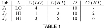
Job L C(LO) C(HI) D C′_(HI)

J1 LO 4 - 10

-J2 HI 1 3 10 2

J3 HI 3 5 10 6

TABLE 1

A Simple Three Job Example

We illustrate the use of this important FO measure via a sim-ple examsim-ple system comprising jobs rather than recurrent tasks. Consider the three jobsJ1, J2, and J3 depicted in Table 1, that

are all released at time-instant zero and have a common deadline at time-instant ten. Suppose that jobJ1is of lower criticality (its

criticality level is “LO” in the terminology of mixed-criticality scheduling theory), while jobsJ2 andJ3are of higher criticality

(i.e., their criticality level is “HI”). Each job is characterized by a LO-criticality execution time estimateC(LO); the HI-criticality jobs have an additional, more conservative HI-criticality execution time estimate C(HI). Under normal (fault-free) execution, all jobs complete within theirC(LO)bounds. The low criticality job is constrained, by run-time monitoring and policing, to execute for no more than itsC(LO)bound. The high criticality jobs can overrun (fail) by executing for more than their respectiveC(LO)

bounds but they are prevented from executing for more than their respectiveC(HI)bounds.

Suppose that the jobs execute in criticality-monotonic or-der – the HI-criticality jobs execute first. Unor-der “traditional” mixed-criticality schedulability analysis (i.e., the analysis inspired by [56]), this system is deemed mixed-criticality schedulable, since

• _{All jobs complete by their deadlines if each job completes} upon executing for no more than their respectiveC(LO)

values, and

• _{The HI-criticality jobs complete by their deadlines} (al-though the LO-criticality job may not) if each job com-pletes upon executing for no more than their respective C(HI)value.

Now consider a second system that differs from the one above in that the C(HI)values are as depicted in the column labeled C′_(HI)

; i.e.,C(HI)is 2 (instead of 3) forJ2and 6 (instead of

5) forJ3. It may be easily verified that this second system is also

mixed-criticality schedulable.

Let us now compute the FO counts for the original and the modified system.

• _{The original system can be seen to have a FO count of 1.} IfJ3 overruns then the execution times could be (for the

three jobs) 4, 1, 5 – so J1, which runs last, completed

by its deadline of 10. Alternatively if J2 overruns the

execution times become 4, 3, 3; so againJ1completed by

its deadline. However, if both high criticality jobs overrun (i.e. FO count would be 2) thenJ1will miss its deadline

as the execution times would be 4, 3, 5.

• For the modified system however, the FO value is 0 since it cannot remain fully operation if jobJ3over-runs, as 4 +

1 + 6>10.

Thus, the original and the modified system are both deemed schedulable in the mixed-criticality sense, but they have different levels of robustness – this difference is not exposed by traditional mixed-criticality scheduling theory. To provide a complete defini-tion of an applicadefini-tion’s survivability, we believe that it is necessary to provide evidence that all deadlines are met during fault free behaviourandprovide a profile of the application’s robustness (as represented by the values of FO count (F) and FR count (M) in this paper).

Run-time response to overload.As stated above, we distinguish between four qualitatively different forms of response that a system may have to a run-time overload, depending upon the severity of the response that is needed: (i) Fully Operational; (ii) Fail Robust; (iii) Fail Resilient; and (iv) Fail Safe/Restart. Different techniques are needed to deal with, and quantitatively analyse, these different forms of survivability.

• Analysis of Fully Operational behaviour requires no changes to the run-time algorithms; instead, careful modi-fication to the scheduling analysis that is performed as part of (pre run-time) verification suffices for determining the FO count.

• _{If an overload becomes severe enough that fully} opera-tional behaviour is not possible, Fail Robust behaviour may be achieved by adopting a disciplined approach to eliminating the overload; this may be achieved by a judicious dropping of jobs of individual robust tasks. • For overloads that are even more severe, Fail Robust

behaviour may not be achievable and strategies must be deployed for further reducing the system load by pro-viding lower-criticality tasks reduced service; the design and analysis of such Fail Resilient response strategies is beyond the scope of this paper, but see the list of references given earlier.

We now discuss our proposed approach towards Fully Operational and Fail Robust behaviours.

Measuring the severity of timing faultsIn this paper we propose the use of a ‘job failure’ (JF) count to represent the (failed) states of the system. If any high criticality job executes for C(LO)

without completion then the count increases (JF := JF + 1).3 Note that we do not distinguish between timing failures from jobs of the same, or from different, high criticality tasks.

To bound the impact of a job failure we assume a maximum execution time of C(HI) for this job. It would be possible to introduce a new parameter,X, which would be an estimate of the maximum overrun of any task (i.e.C(LO)< C(X)< C(HI)), but in this initial study we restrict ourselves to the simpler model (see discussion in Section 9).

With this framework an application is able to define its level of robustness. In the following we use F to represent the FO value and M the FR value. An example of the framework is: Fail Operational when JF ≤ F = 3, and Fail Robust when

3 < JF ≤M = 6. Only resorting to resilience strategies such as period extending or task dropping whenJF > 6. Analysis, see Section 5, can be used to verify that the system can deliver behaviour that satisfies the F andM parameters. This analysis can also be used to determine the maximum time it would take for a system experiencingM concurrent faults to experience an idle tick (which resetsJF to zero). This allows the common form for expressing reliability, “number of faults to be tolerated in a defined time interval”, to be used.

An orthogonal Reliability Model [14] may be used to assign a probability to the likelihood of experiencingJF > 6 in, say, an hour of operation. Hence the level of tolerance of concurrent transient timing faults can be tuned to meet the needs of the application. More severe or permanent faults will need more extreme responses involving significant degradation or recovery at a system level (through, for example, channel replication or transition to a safe state). Here we allow robustness in the face of rare transient timing faults to be delivered by employing a mixed-criticality approach.

This paper does not attempt to provide guidance on what the Fail Operational (F) and Fail Robust (M) values should be. Various application-specific factors will impact on these values, including the consequences of a timing failure, and the level of redundancy provided at the system level. Both FMEA (Failure Modes and Effect Analysis) and FTA (Fault Tree Analysis) [48] can be employed to help determineFandM. Rather, the analysis provided in this paper allows schedulability to be checked once these values are identified, or the level of robustness determined for a specified system. In the remainder of this paper (after the Related Work section) we illustrate how existing analysis for fixed priority mixed-criticality systems can be adapted to provide these checks. However this analysis is not the main focus of the paper; rather it is included to demonstrate that our model of robustness is amenable to analysis. Its incorporation within other scheduling frameworks should be straightforward.

3

RELATED

WORK

Research into soft real-time systems deals with issues of minimis-ing the latency of responses, minimisminimis-ing the number of deadline

3. However, whenever the system experiences an idle tick (or idle instant – anidle instantis a point in time when there are no jobs released strictly before that time which have execution time remaining) the count is set back to zero (J F:= 0).

misses, supporting value added computation such as that provided by imprecise computations [38], [49], best-effort scheduling [39], and overload management [33]. By comparison, a hard real-time system is designed to meet all of its deadlines in a well-defined worst-case set of circumstances. We note that this requirement is not contradicted by the added constraint of providing robust or resilient behaviour when this worst-case set of circumstances is violated and timing overruns occur. A robust hard real-time system is thus not a soft real-time system; however, some of the techniques developed for soft real-time systems may be applicable. There are a number of approaches that bridge between hard and soft real-time behaviours. Koren and Shasha [34] introduced the idea of allowing some jobs of a task to be skipped, according to a skip-factor. Them-kfirm scheme of Ramanathan [25], [44] predefines specific jobs of a task as optional, with the scheduling algorithm running them at a lower priority, thus ensuring schedu-lability (hard real-time behaviour) of only the mandatorym out ofkjobs. The weakly-hard scheme of Bernat et al. [8] generalises requirements for the jobs of a task that must meet their deadlines according to a statically defined profile, such as requiring that at leastnout of anymjobs must meet their deadlines.

More closely related to the research presented in this paper is the concept of Window-Constrained execution time Systems (WCS); also aimed at hard real-time systems. In WCS, tasks are allowed a profile of execution times that can include overruns. For example a task with a worst-case execution time of 12 ticks can have a profile that allows it to execute for 14 ticks in any two out of four jobs. Balbastre et al. [2], [3] provide schedulability analysis for WCS based on EDF scheduling.

The key difference between work on WCS (and others men-tioned above) and that presented in this paper, is that here we consider the impact of overruns for Fail Operational or Fail Robust overallof the (HI-criticality) tasks taken together. In other words we see robustness as a property of the whole system, not of each system task.

Thus the offline analysis derived in this paper for fixed priority mixed-criticality based scheduling combines with a simple online mechanism to support robust and gracefully degrading behaviour at runtime when it is not known which jobs of which tasks will exhibit execution time overruns. Such overruns are expected to occur only rarely, but nevertheless could be clustered due to common causes (e.g. jobs of multiple tasks running error-handling code due to an invalid sensor reading). Here, we are not looking at particular task profiles but rather we address overruns in the set of executing tasks as a whole. So, for example, we may require a system to remain schedulable if at most three jobs overrun, but not more than three, and not any particular three. Hence, in this case, the three overrunning jobs may belong to any one, two, or three tasks in the system. Moreover, we allow jobs of robust tasks to be skipped to provide a controlled form of graceful degradation. WCS does not cater for these behaviours.

Another form of controlled degradation is proposed by Gu and Easwarn [23]. They allow HI-criticality tasks to share a budget, and thereby postpone the time when LO-criticality tasks need to be dropped. Their approach however has a number of run-time complexities and is only applicable to systems scheduled using the EDF scheme. They also do not allow particular levels of robustness to be verified; nor do they allow job skipping.

how far a schedulable system is from becoming unschedulable. Typically a critical scaling factor (cf > 1) is derived such that if all task execution times are multiplied bycf then the system remains schedulable, but if any factor cf′ _{> cf}

is used then the system becomes unschedulable. Sensitivity analysis is used as part of the design process to manage risk (it allows potential problems to be anticipated). In this paper we are using analysis to judge how many errors (job overruns) can be accommodated, and how many jobs need to be skipped to bound the impact of job overruns. Sensitivity analysis is also used by Burns et al. [14] to determine how many functional errors a system can tolerate. Here a functional error will result in extra computation (an exception handler, recovery block, or re-execution from a checkpoint [42]). This is therefore a different fault model to the one addressed in this paper which considers temporal faults.

4

SYSTEM

MODEL

In this paper we illustrate how the defined notion of robustness can be incorporated into Fixed Priority Preemptive Scheduling (FPPS) of a mixed-criticality system comprising a static set of n sporadic tasks which execute on a single processor. We have chosen fixed priority-based scheduling as this is used in safety-critical industries such as avionics [7], [29]. We assume a discrete time model in which all task parameters are given as integers. Each task, τi, is defined by its period (or minimum arrival interval), relative deadline, worst-case execution time, level of criticality, and unique priority: (Ti,Di,Ci,Li,Pi). In addition, a Boolean value indicates whether the task is robust or not, i.e. can have a job skipped. We restrict our attention to constrained-deadline systems in whichDi ≤Tifor all tasks. Further, we assume that the processor is the only resource that is shared by the tasks, and that the overheads due to the operation of the scheduler and context switch costs can be bounded by a constant, and hence included within the worst-case execution times attributed to each task.

We assume that each task τi gives rise to a potentially un-bounded sequence of jobs, with the release of each job separated by at least the minimum inter-arrival time from the release of the previous job of the same task. The worst-case response time of taskτiis denoted byRiand corresponds to the longest time from release to completion for any of its jobs. A task is referred to as schedulable if its worst-case response time does not exceed its deadline.

Note in the remainder of the paper we drop the task index in general discussions where it is not necessary to distinguish between parameters of different tasks.

The system is assumed to be defined over two criticality levels (HI andLO) (extension to more levels is discussed in Section 9). Each LO-criticality task is assumed to have a single estimate of its WCET:C(LO); each HI-criticality task has two estimates: C(HI)andC(LO), withC(HI) ≥C(LO), and by definition the differenceC(DF) =C(HI)−C(LO). It follows that a HI-criticality task also has two estimates of its utilisation:C(HI)/T (its HI-criticality utilisation) and C(LO)/T (its LO-criticality utilisation). The implementation platform is a uniprocessor, al-though the approach developed is applicable to multiprocessor platforms with partitioned tasks.

Most scheduling approaches for mixed-criticality systems identify different modes of behaviour. In the LO-criticality (or normal) mode, all tasks execute within theirC(LO)bounds and

all deadlines are guaranteed to be met. In the HI-criticality mode, however, only the HI-criticality tasks are guaranteed as some of these tasks have executed beyond C(LO) (although no higher thanC(HI)). At all times LO-criticality tasks are constrained by run-time monitoring to execute for no more than their C(LO)

bound. If any HI-criticality task attempted to execute for more thanC(HI)then the fault is of a more severe nature and system-level strategies such as Fail Stop or Fail Restart must be applied. The current scheduling scenario is abandoned.

As the C(LO) bounds are intended to be sufficient for all tasks, any HI-criticality job that executes for more thanC(LO)is deemed to have failed in the temporal domain. The job however continues to execute and will complete successfully, assuming its C(HI)bound is respected.

The response time of a task in LO-criticality mode is denoted byR(LO)and in HI-criticality mode byR(HI).

5

ANALYSIS FOR A

FIXED

PRIORITY

INSTANTIA-TION OF THE

FRAMEWORK

As indicated above, we demonstrate that the proposed framework can be incorporated into a scheduling scheme, with relevant analysis, by focusing on fixed priority based scheduling and by extending AMC analysis [5]. This AMC analysis has become the standard approach to apply to mixed criticality systems imple-mented upon a fixed priority based platform.

5.1 Original AMC Analysis

Before any level of robustness is considered the task set must be passed as schedulable. This analysis has three phases:

1) Verifying the schedulability of the LO-criticality (normal) mode,

2) Verifying the schedulability of the HI-criticality mode, 3) Verifying the schedulability of the mode change itself.

First the verification (for all tasks) of the LO-criticality mode is undertaken:

Ri(LO) = Ci(LO) + X

j∈hp(i)

Ri(LO)

Tj

Cj(LO) (1)

wherehp(i)is the set of all tasks with priority higher than that of taskτi.

This response-time equation (and the others in the paper), is solved in the standard way by forming a recurrence relation (fixed point iteration).

Next the HI-criticality mode:

Ri(HI) = Ci(HI) + X

j∈hpH(i)

Ri(HI)

Tj

Cj(HI) (2)

wherehpH(i)is the set of HI-criticality tasks with priority higher than or equal to that of taskτi– we also usehpL(i)to denote the set of LO-criticality tasks with priority higher than or equal to that of taskτi. NoteRi(HI)is only defined for tasks of HI-criticality.

For the mode change itself:

Ri(HI∗

) = Ci(HI) + X

τj∈hpH(i)

Ri(HI∗

)

Tj

Cj(HI) +

X

τk∈hpL(i)

Ri(LO)

Tk

this ‘caps’ the interference from LO-criticality tasks. Note Ri(HI∗

) ≥ Ri(LO), and Ri(HI∗

) ≥ Ri(HI), hence only equations (1) and (3) need be applied.

We are now able to derive analysis for Fail Operational and Fail Robust. It is assumed that the task set is fully defined, priorities are assigned and the two levels of robustness are fixed:

F Number of HI-criticality job overruns that must be tolerated without any performance degradation. M Number of HI-criticality job overruns that must be

tolerated with at most one job being skipped per robust task.

As noted earlierM ≥F.

5.2 Fail Operational Analysis

For Fail Operational behaviour, up to F HI-criticality jobs are allowed to execute up to theirC(HI)values. This will result in extra load on all tasks in the LO-criticality mode:

Ri(F) = LD(Ri(F), F) + Ci(LO) +

X

j∈hp(i)

_Ri(F)

Tj

Cj(LO) (4)

where LD(Ri(F), F) is the extra load in the response time Ri(F)from up toF HI-criticality jobs of priorityPi or higher executing forC(HI)rather thanC(LO).

We define LD using amultiset (orbag), BG. The multiset contains theCj(DF)(i.e.Cj(HI)−Cj(LO)) values of tasks that have the following properties:

Lj=HI ∧ Pj≥Pi

The multiset contains theCj(DF)value l_R

i(F)

Tj

m

times. LDis then the sum of theF largest values inBG. Note when analysing response times, for some tasks (especially high priority ones)BG may contain fewer elements than the parameterF. In this case LDis simply the sum of all the elements inBG.

OnceR(F)is computed, the mode change can be considered. This requires an update to equation (3), since the move to the HI-criticality mode has been postponed and hence the ‘capping’ of LO-criticality work during the transition to the HI-criticality mode needs to be modified:

Ri(HI∗

) = Ci(HI) + X

τj∈hpH(i)

Ri(HI∗

)

Tj

Cj(HI) +

X

τk∈hpL(i)

Ri(F)

Tk

Ck(LO) (5)

5.3 Fail Robust Analysis

Assuming a system is schedulable with the particularJF value of F, the next requirement for Fail Robustness is forJF to increase toM (M for maximum number of job failures to be tolerated). With this behaviour, all robust tasks can drop a job once JF exceedsF. So if such a task is released at least once afterR(F)

then a job can be skipped. We model this by adding a new term that reduces the load:

Ri(M) = LD(Ri(M), M) + Ci(LO) +

X

j∈hp(i)

_Ri(M)

Tj

−Sj

Cj(LO) (6)

whereSjequals 1 if the task is robustand

_Ri(M)

Tj

>

_Ri(F)

Tj

(7)

otherwise it is 0. The functionLDis as defined for equation (4), but forM HI-criticaility jobs.

Note this straightforward formulation is potentially pessimistic in that a skipped task could still be a member of BG and contributeC(DF)to the load even thoughC(LO)is being with-drawn. To remove this pessimism the number of timesCj(DF)

is placed inBGis reduced to l_R

i(M)

Tj

m

−Sj.

As no skipping can occur beforeR(F)we can conclude that R(M)≥R(F). We must therefore again modify equation (3):

Ri(HI∗

) = Ci(HI) + X

τj∈hpH(i)

Ri(HI∗

)

Tj

Cj(HI) +

X

τk∈hpL(i)

_Ri(M)

Tk

Ck(LO) (8)

The analysis given in equation (8) is likely to be pessimistic, but can be improved upon (as shown in equation (9)) by account-ing for the jobs that are skipped if the system moved to the HI-criticality mode from the robust mode (see also Section 7):

Ri(HI∗

) = Ci(HI) +

X

τj∈hpH(i)

Ri(HI∗

)

Tj

−SH j

Cj(HI) +

X

τk∈hpL(i)

Ri(M)

Tk

−SL k

Ck(LO) (9)

Here, the definition ofSis extended;SL

j is defined using equation (7) whereasSH

j takes the value 1 if the task is robustand:

_Ri(HI∗₎

Tj

>

_Ri(F)

Tj

Note a robust task that has not dropped a job before the move to the HI-criticality mode can still do so. The above analysis benefits from this behaviour.

5.4 ChoosingFandM – a Pareto Front

A system designer must trade off schedulability and robustness; however, robustness can be achieved by fail operational and/or fail robust behaviour. Fail operational is clearly preferred, but the maximum overall robustness is not necessarily achieved by first maximisingF and then maximisingM. For example, a task set may be schedulable withF=1,M=8 or withF=2,M=4. Which is best is clearly a design issue, but the choice is of a common form known as aPareto front.

Consider the analysis derived above, from equation (4),R(F)

is monotonically non-decreasing inF. Further, from equations (6), (7) and (9),R(M)is monotonically non-decreasing inR(F). It follows that forF′ _{> F}

, then the maximum supported valuesM′ andM have the relationship:M ≥ M′

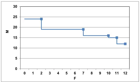
0 5 10 15 20 25 30

0 1 2 3 4 5 6 7 8 9 10 11 12

M

F

Fig. 1. Pareto Optimal Choices

number of optimal pairings that the designer should choose. This can be illustrated by an example.

A randomly generated system with 20 tasks and LO-criticality utilisation of 0.75 was analysed by choosing values of F from 0 to 13 (at which point the task set is unschedulable). For each value ofF the maximum value ofM is computed via a binary search. The task set is itself a typical example of those generated during the evaluation experiments reported in Section 8. Figure 1 shows the Pareto optimal choices. At one extreme ifF is set at 0 then 24 overruns can be accommodated by job skipping. At the other extrene, if F is set to 12 then no further robustness can be achieved, skipping adds nothing. In all there are 5 Pareto optimal combinations ofF andM: (2,24), (7,19), (10,16), (11,15) and (12,12). The designer must choose one, remembering that the choice is influenced by how close together job skipping is allowed. A highM, due to a lowF, will increase the likelihood of a move to the robust mode. This will then increase the possibility of such events being too close together – see discussion in Section 7.

A final point to note is that if F andM are given then the analysis can be used to compute the number of robust tasks that would be required to deliver these values. This might be a useful number to know, but whether a task is robust or not is a property of its semantics and would not be an easy property to add during system integration (when the scheduling analysis is undertaken).

5.5 Example task set

To illustrate the use of the above analysis a simple example is presented below. Consider the three task system defined in the following table. The aim here is to maximiseF and thenM.

τi L P C(LO) C(HI) T =D

τ1 HI 1 1 4 5

τ2 LO 2 4 - 20

τ3 HI 3 1 2 30

For each task response times can be computed: Rwhich ig-nores criticality and assumes each task executes forC(L),R(LO)

which assumes each task executes forC(LO)andR(HI∗

)which is delivered by AMC and equation (3). These values are as follows:

τi R R(LO) R(HI∗₎

τ1 4 1 4

τ2 20 5

-τ3 ∞ 7 30

Note τ3 is unschedulable without the use of mixed-criticality

scheduling. We can now compute the response times for each task when there areF job overruns. Two values need to be computed: R(F)andR(HI∗

)for that value ofF. Equations (4) and (5) are used for this purpose to give the following results. Note thatτ3is

not schedulable withF = 4, sinceR(HI∗₎

exceeds its deadline.

τi R(1) R(HI∗

) R(2) R(HI∗

)

τ1 4 4 4 4

τ2 9 - 13

-τ3 10 30 14 30

τi R(3) R(HI∗

) R(4) R(HI∗

)

τ1 4 4 4 4

τ2 17 - 20

-τ3 18 30 27 34+

For example consider R3(F = 3), starting with an initial

estimate of 14 (asR(3)≥R(2)). Within 14 ticks there have been three releases of τ1 and one release of τ3, hence BG contains {3,3,3,1} giving an LD term of 9 (i.e. the sum of the three largest values withinBG). Equation (4) thus becomes:

R3(3) = 9 + 1 +

₁₄

5

1 +

₁₄

20

4 = 17

one more iteration gives 18, and then:

R3(3) = 9 + 1 +

₁₈

5

1 +

₁₈

20

4 = 18

Equation (5) then becomes:

R3(HI∗) = 2 +

R3(HI∗) 5

4 +

18 20

4

which has the solution 30.

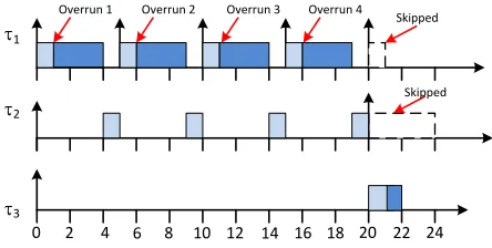
The analysis shows that this task set can survive three job over-runs with no missed deadlines. However, to push the robustness further, a fourth job overrun can only be accommodated by job skipping. This assumes thatτ1 andτ2 are robust, and that they

have not skipped a recent job. Consider the required behaviour whenM=4 forτ3. First we computeR3(4)using equation (6). If

we start the iterative solution withR3(4)=R3(3)=18 then there is

no skipping and we computeR3(4)=21. Now with the value of

21, the relationship contained in equation (7) is true for bothτ1

andτ2and hence both of these tasks have a value ofSthat is 1.

So each of these tasks drops a job and R3(4)remains with the

value 21. The final step is to computeR3(HI∗); from equation

(9) we have:

Ri(HI∗

) = 2 +

_Ri(HI∗₎

5

−1

4 +

₂₁

20

−1

4

which has the solution 22. The fourth job overrun must occur before time 20, and hence the fifth release ofτ1 and the second

1

3

2 4 6 8 10 12 20 22

0 24

2

14 16 18

Skipped Overrun 1 Overrun 2 Overrun 3 Overrun 4

Skipped

Fig. 2. Fail Robust schedule for Example Task Set

6

ROBUST

PRIORITY

ASSIGNMENT

Vestal [56] showed that deadline monotonic priority assignment is not optimal for schemes in which tasks have more than one ‘worst-case execution time’ (i.e.C(LO)andC(HI)).

For the system model and analysis derived in this paper, we now show that Audsley’s priority assignment algorithm [1] is applicable. This algorithm first identifies some task which may be assigned the lowest priority; having done so, this task is effectively removed from the task set and priority assignment is recursively obtained for the remaining tasks. The advantage of applying Audsley’s algorithm is that it delivers an optimal assignment in a maximum ofn(n+ 1)/2task schedulability tests. If the algorithm were not applicable then an exhaustive search over alln!possible priority orderings would potentially be required.

For the analysis derived in Section 5 it is straightforward to confirm that Audsley’s algorithm is still applicable. To do this it is sufficient to demonstrate that the following conditions hold for the applied schedulability test, Z [16]:

1) The schedulability of a task may, according to test Z, be dependent on the set of higher priority tasks, but not on the relative priority ordering of those tasks.

2) The schedulability of a task may, according to test Z, be dependent on the set of lower priority tasks, but not on the relative priority ordering of those tasks.

3) When the priorities of any two tasks of adjacent priority are swapped, the task being assigned the higher priority cannot become unschedulable according to test Z, if it was previously schedulable at the lower priority. (As a corollary, the task being assigned the lower priority cannot become schedulable according to test Z, if it was previously un-schedulable at the higher priority).

For fixed values ofF andM then an inspection of equations (4) & (5) and (6) & (9) and the definitions ofLDandBGshows that indeed these three conditions hold, and hence an optimal static priority ordering can be obtained using Audsley’s algorithm.

Note that if the analysis is being used to estimate the robust-ness of a given system (i.e. for a fully specified task set what values ofF andM can be sustained) then a simple scan over the values of F and a binary search for the maximum M (for a given F) can be used to determine the Pareto Front and each Pareto Optimal pair of values.

We note that for each iteration, the optimal priority ordering must be re-computed as it will depend on the particular values of F andM.

7

RUN-TIME

BEHAVIOUR

It is important that any scheme developed for improving system robustness must itself be straightforward and efficient. It must not add, in any significant way, to the complexity or run-time overheads of the system’s implementation. We have focussed our attention on fixed-priority based scheduling as this has industrial application in the safety-critical field [7], [29]. And in these appli-cation areas run-time monitoring is used, and indeed mandated.

To ensure necessary temporal isolation between different crit-icality levels some form of run-time monitoring is required. At a minimum this will prevent any LO-criticality job from executing for more than its WCET bound, i.e. C(LO). Given that this monitoring is already a requirement, it is a minor addition to also require that HI-criticality jobs are monitored. This monitoring will both check that the C(HI)bound is not infringed and keep a count of the number of HI-criticality jobs which have overrun; i.e. executed beyondC(LO).

The analysis developed in Section 5 allows the two parameters F andM to be determined. If more thanF HI-criticality jobs have overrun then the system’s criticality mode is changed from

normal to robust. In this mode the next job of all robust tasks is skipped. Subsequently if more than M HI-criticality jobs overrun the system’s criticality mode changes to HI-criticality. Now significant degradation must occur, LO-criticality work may need to be dropped. As indicated in Section 2, there are a number of possible strategies published for managing this behaviour and providing increased system resilience. In this paper we do not attempt to evaluated these schemes; the most appropriate will clearly be application dependent.

At any idle instant,t, the count of job overruns is re-set to 0, and the system’s criticality mode is returned to eithernormalor

normal-no-skip. If all robust tasks are ready to skip (again) the system goes back tonormal, otherwise it goes tonormal-no-skip. While innormal-no-skipmode up toF faults can be tolerated, but no job skipping is allowed. IfF+1 faults occur in this mode then the system’s criticality mode changes directly to HI-criticality. When the system returns tonormalornormal-no-skipmodes then a task that is marked as ‘skip next job’ but which has not yet released that job, no longer needs to degrade. Its next job does not need to be skipped.

It is assumed in this work that the C(LO) estimates for both LO- and HI-criticality tasks have been produced with sound engineering techniques. Hence any overrun is effectively a timing fault and will be a rare event in a well-tested system. It follows that F overlapping faults and the move to therobust mode will happen very rarely if at all.

As discussed in Section 2 a Reliability Model can be used to assign a probability to the possibility of more than M concur-rent faults occurring within a defined interval. In the evaluation reported in the next section, we therefore focus on isolated fault sequences.

8

EVALUATION

look at all possible permutations of 3 faults from up to 30 jobs to ensure that the worst case has been covered (30, as 3 faults could come from 3 executions of 1 task, or 2 from 1 and 1 from another, or 3 from any of the 10 tasks). This lack of applicability of other schemes means that an evaluation based on an exploration of different algorithms and methods would not be valid or useful. The criteria for comparison (improved robustness as defined in this paper) cannot be defined for other schemes that have been derived with other criteria in mind. Moreover, our use of fixed priority based scheduling, as apposed to EDF, which a number of other approaches adopt, makes a direct comparison impossible. In terms of industrial usage a fixed priority based approach is more appropriate than EDF (which has currently little/no application in the high criticality arena; although this may change in the future). The evaluations reported in this section therefore address the trade-off between schedulability and robustness. The experiments consider, over a wide range of system and task parameters, the decrease in schedulability that results from various levels of robustness as defined by the two parametersF andM.

8.1 Taskset parameter generation

The task set parameters used in our experiments were randomly generated as follows:

• Task utilisations (Ui =Ci/Ti) were generated using the UUnifast algorithm [9], giving an unbiased distribution of utilisation values.

• Task periods were generated according to a log-uniform distribution with a factor of 100 difference between the minimum and maximum possible task period. This repre-sents a spread of task periods from 10ms to 1 second, as found in many hard real-time applications.

• _{Task deadlines were set equal to their periods.}

• _{The LO-criticality execution time of each task was set} based on the utilisation and period selected:Ci(LO) =

Ui/Ti.

• _{The HI-criticality execution time of each task was a fixed} multiplier of the LO-criticality execution time,Ci(HI) =

CF·Ci(LO)(e.g.,CF = 2.0).

• _{The probability that a generated task was a HI-criticality} task was given by the parameterCP (e.g.CP = 0.5). • The probability that a generated task was skippable was

given by the parameterSP (e.g.SP = 0.5).

The values over which these parameters range are informed by industrial practice [35].

8.2 Schedulability tests investigated

We investigated the performance of the following techniques and associated schedulability tests. In all cases, Audsley’s algorithm was used to provide optimal priority assignment [1].

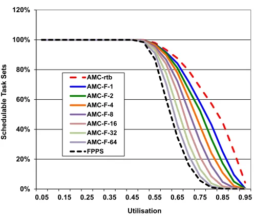
• AMC-rtb: This is the standard schedulability test for AMC [5] given by (1) and (3) in Section 5.

• _{AMC-F-xx: This is the test for Fail Operational behaviour,} given by (4) and (5), with a value ofF equal toxx. • _{AMC-M-yy: This is the test for Fail Robust behaviour,}

given by (6) and (9), with a value ofM equal toyy. (Note this analysis first checks that the system is Fail Operational withF = 0i.e. schedulable according to AMC-rtb).

0% 20% 40% 60% 80% 100% 120%

0.05 0.15 0.25 0.35 0.45 0.55 0.65 0.75 0.85 0.95

S

c

h

e

d

u

la

b

le

T

a

s

k

S

e

ts

Utilisation AMC-rtb

AMC-F-1 AMC-F-2 AMC-F-4 AMC-F-8 AMC-F-16 AMC-F-32 AMC-F-64 FPPS

Fig. 3. Schedulability for Fail Operational

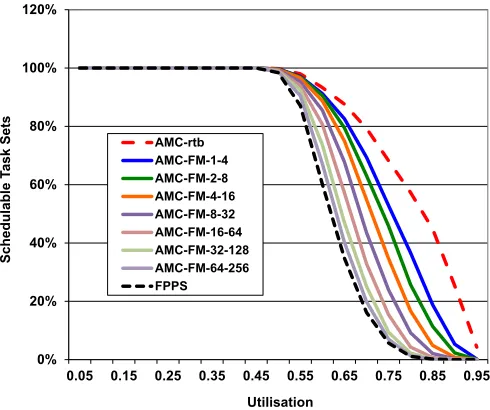
• _{AMC-FM-xx-yy: This is the test for both Fail Operational} and Fail Robust behaviour, with values ofF = xx, and M =yy.

• FPPS: This is an exact test for FPPS (standard Fixed Priority Preemptive Scheduling). It checks if the system is schedulable when all LO-criticality tasks execute for C(LO) and all HI-criticality tasks execute for C(HI)

(i.e. it ignores, and therefore does not exploit, the fact that the task set is mixed criticality).

8.3 Baseline Experiments

In our baseline experiments, the task set utilisation was varied from 0.05 to 0.954_{. For each utilisation value, 1000 task sets were}

generated and the schedulability of those task sets determined using the algorithms / schedulability tests listed above. The graphs are best viewed online in colour.

Figure 3 plots the percentage of task sets generated that were deemed schedulable for a system of 20 tasks, with on average 50% of those tasks having HI-criticality (CP = 0.5) and each task having a HI-criticality execution time that is 2.0 times its LO-criticality execution time (CF = 2.0). The various solid lines in Figure 3 show Fail Operational schedulability for increasing values of F. Note that these lines have a strict dominance relationship between them. They are dominated by AMC-rtb (which is effectivelyF = 0) and they dominate FPPS (which is effectivelyF =∞). We observe that there is a degradation in schedulability as support is added for an increasing number of overruns; for example at utilisation of 0.8 schedulability forF = 0is approximately 60%, whereas for F = 2, it has dropped to (again approximately) 38%. However, if the advantages obtained from a mixed criticality approach are ignored the level of schedulability is close to zero.

Figure 4 uses the same task set configurations as Figure 3; however, it shows Fail Robust schedulability for increasing values of M, assuming that F = 0. Note the probability that each generated task was marked as ‘skippable’ was set toSP = 0.5. Again, supporting an increasing number of overruns leads to a degradation in schedulability; however, due to the processor time

0% 20% 40% 60% 80% 100% 120%

0.05 0.15 0.25 0.35 0.45 0.55 0.65 0.75 0.85 0.95

S

c

h

e

d

u

la

b

le

T

a

s

k

S

e

ts

Utilisation AMC-rtb

AMC-M-1 AMC-M-2 AMC-M-4 AMC-M-8 AMC-M-16 AMC-M-32 AMC-M-64 FPPS

Fig. 4. Schedulability for Fail Robust

0% 20% 40% 60% 80% 100% 120%

0.05 0.15 0.25 0.35 0.45 0.55 0.65 0.75 0.85 0.95

S

c

h

e

d

u

la

b

le

T

a

s

k

S

e

ts

Utilisation AMC-rtb

AMC-FM-1-4 AMC-FM-2-8 AMC-FM-4-16 AMC-FM-8-32 AMC-FM-16-64 AMC-FM-32-128 AMC-FM-64-256 FPPS

Fig. 5. Schedulability for Fail Robust combined with Fail Operational

freed up by skipping jobs, this degradation is substantially less than in Figure 3.

Figure 5 combines analysis of both Fail Operational and Fail Robust behaviour, showing how schedulability degrades for increasing values of F andM, with M set to4F. Comparing Figure 3 and Figure 5, we observe that due to the skipping of jobs (noteSP = 0.5), adding Fail Robust comes at a relatively small cost in terms of schedulability.

8.4 Weighted Schedulability Experiments

In the following figures we show the weighted schedulability measure Wz(p) [6] for schedulability test z as a function of parameterp. For each value ofp, this measure combines results for all of the task setsτgenerated for all of a set of equally spaced utilization levels (0.05to0.95in steps of0.05).

LetSz(τ, p)be the binary result (1 or 0) of schedulability test zfor a task setτ with parameter valuep:

0.00 0.10 0.20 0.30 0.40 0.50 0.60 0.70 0.80 0.90 1.00

0.5 1 1.5 2 2.5 3 3.5 4

W

e

ig

h

te

d

S

c

h

e

d

u

la

b

il

it

y

Range of task periods 10r

AMC-rtb AMC-FM-1-4 AMC-FM-2-8 AMC-FM-4-16 AMC-FM-8-32 AMC-FM-16-64 AMC-FM-32-128 AMC-FM-64-256 FPPS

Fig. 6. Weighted Schedulability: Range of task periods

Wz(p) = (X

∀τ

u(τ)·Sz(τ, p))/X ∀τ

u(τ) (10)

whereu(τ)is the utilization of task setτ.

The weighted schedulability measure reduces what would otherwise be a 3-dimensional plot to 2 dimensions [6]. Weighting the individual schedulability results by task set utilization reflects the higher value placed on being able to schedule higher utilization task sets.

We show how the results are changed by varying each of the key parameters (one at a time). Figure 6 varies the range of task periods, Figure 7 varies the Skip Proportion (SP), Figure 8 varies the Criticality Proportion (CP), Figure 9 varies the Criticality Factor (CF), and finally Figure 10 varies the number of tasks. In each of the experiments, we explored schedulability for combined Fail Operational and Fail Robust behaviour.

Figure 6 illustrates how the weighted schedulability measure varies with the range of tasks periods. For a small range of periods of 100.5 _{≈ 3.16 then values of F ≥ 16 are enough}

that almost all overruns that could possible take place in a busy period are accounted for, and thus schedulability is effectively the same for AMC-FM-16-64, AMC-FM-32-128, and AMC-FM-64-256 as it is for FPPS. As the range of task periods increases then differences appear, since there may be many jobs in the longest busy period. At the extreme with a range of task periods of 4 orders of magnitude, then 64 overruns is a relatively small number in comparison to the total number of jobs in the busy period for low priority tasks and thus AMC-FM-64-256 has significantly better performance than FPPS.

0.00 0.10 0.20 0.30 0.40 0.50 0.60 0.70 0.80 0.90 1.00

0.05 0.15 0.25 0.35 0.45 0.55 0.65 0.75 0.85 0.95

W e ig h te d S c h e d u la b il it y

Skip Proportion (SP)

AMC-rtb AMC-M-1 AMC-M-2 AMC-M-4 AMC-M-8 AMC-M-16 AMC-M-32 AMC-M-64 FPPS

Fig. 7. Weighted Schedulability: Skip Proportion (SP)

0.00 0.10 0.20 0.30 0.40 0.50 0.60 0.70 0.80 0.90 1.00

0.05 0.15 0.25 0.35 0.45 0.55 0.65 0.75 0.85 0.95

W e ig h te d S c h e d u la b il it y

Criticality Proportion (CP) of HI-Criticality AMC-rtb AMC-FM-1-4 AMC-FM-2-8 AMC-FM-4-16 AMC-FM-8-32 AMC-FM-16-64 AMC-FM-32-128 AMC-FM-64-256 FPPS

Fig. 8. Weighted Schedulability: Criticality Proportion (CP)

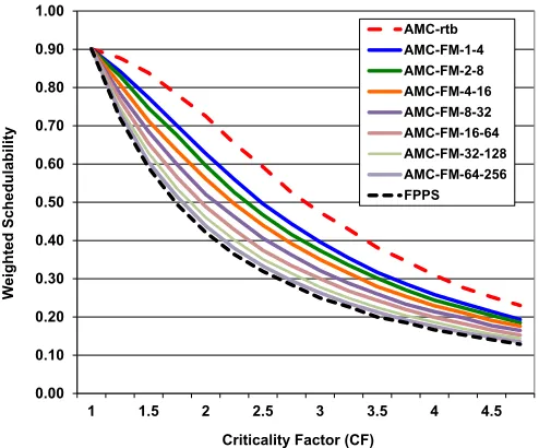
Figures 8, 9, and 10 illustrate respectively how the weighted schedulability measure varies with the probability that a gener-ated task is HI-criticality (CP), the Criticality Factor (CF =

C(HI)/C(LO)), and the number of tasks. In all cases the performance of the combined Fail Operational and Fail Robust analysis provides an intermediate level of schedulability, degraded from that of AMC-rtb, while improving upon FPPS. We observe that in Figure 10 that when there are very few tasks, the lines for larger values ofF approach the line for FPPS. This is because the number of overruns which need to be supported Fail Operational exceed the maximum number of job releases in a busy period, hence the analysis reduces to the same as FPPS.

0.00 0.10 0.20 0.30 0.40 0.50 0.60 0.70 0.80 0.90 1.00

1 1.5 2 2.5 3 3.5 4 4.5

W e ig h te d S c h e d u la b il it y

Criticality Factor (CF)

AMC-rtb AMC-FM-1-4 AMC-FM-2-8 AMC-FM-4-16 AMC-FM-8-32 AMC-FM-16-64 AMC-FM-32-128 AMC-FM-64-256 FPPS

Fig. 9. Weighted Schedulability: Criticality Factor (CF)

0.00 0.10 0.20 0.30 0.40 0.50 0.60 0.70 0.80 0.90 1.00

8 16 24 32 40 48 56 64 72 80

W e ig h te d S c h e d u la b il it y

Number of Tasks AMC-rtb AMC-FM-1-4 AMC-FM-2-8 AMC-FM-4-16 AMC-FM-8-32 AMC-FM-16-64 AMC-FM-32-128 AMC-FM-64-256 FPPS

Fig. 10. Weighted Schedulability: Number of tasks

9

EXTENSIONS TO THE

BASIC

MODEL

In this section we look at extensions to the basic model derived above. We consider more than two criticality levels and a finer grained monitoring of job overruns.

9.1 More than two criticality levels

Two distinct criticality levels, and one non-critical level, is a common use case.

In Vestal’s original paper [56] all tasks had execution-time estimates for all criticality levels, implying for five levels, five estimates for each task. Later studies [4] restricted this to require estimates only for the criticality level of the task and all levels below. A further restriction [11], [40] is to require only two estimates, one for the task’s criticality level and one for the lowest criticality level in the system.

The number of job timing failures allowed (the F and M parameters used earlier in the paper) could be defined in terms of any job executing beyond criticality level bounds. For example, using Vestal’s model and five criticality levels: L1 (lowest) to

L5 (highest): a value for F of 4 would include either four

jobs executing for more than C(L1) but less than C(L2), or

one job executing for more than C(L1) but less than C(L5)

(or any intermediate combination leading to the overrun of four boundary values). A simple run-time count of overruns is all that is required. The analysis for two criticality levels extends in a straightforward way to any number of levels (just as the standard AMC analysis does [18]). With the dual-criticality model whenM is exceeded then this indicates a serious overrun and LO-criticality tasks are abandoned in order to protect HI-criticality work. With five criticality levels then a series of increasingM values can be derived (M1,M2,M3,M4). Now ifM1is exceededL1tasks

are abandoned, ifM2is subsequently exceeded thenL2tasks are

abandoned, etc. In the extreme (highly unlikely) case, ifM4is exceeded then only the highest criticality tasks (L5) are retained.

9.2 Finer grained job monitoring

The model derived in detail in this paper assumes that if a job of a HI-criticality task overruns its C(LO)estimate then it will execute for C(HI). This is however a pessimistic assumption. An overrun is much more likely to be marginal with the job completing well before itsC(HI)estimate. A number of alter-native formulations are easily derived following the framework developed in this paper. For example, an overrun quantum,C(O)

could be defined; with the F and M parameters counting the number of such exceedances. So a HI-criticality task that does not complete by C(LO)is initially assumed (for a single overrun) to execute forC(LO) +C(O). If it still has not competed after executing for C(LO) +C(O), then a second overrun is noted and an execution time of C(LO) + 2C(O) is assumed, and so on. The analysis developed in Section 5 can easily be modi-fied to accommodate this finer grained monitoring (by replacing C(DF) =C(HI)−C(LO)withC(O)).

10

CONCLUSION

This paper has focused on improving the robustness of mixed-criticality systems. Although software components and their tasks can be assigned criticality levels, this does not mean that every job of a task has that level of importance. Many tasks are naturally robust to the occasionally missing or late job (or can be designed to be so).

Worst-case execution time analysis and the appropriate schedulability analysis allows the timing properties of a system to be verified. For most high integrity applications this is a necessary but not sufficient condition for deployment. A system must also be able to demonstrate that it is tolerant of failures, both permanent and transient. Most timing faults are transient. They manifest

themselves as job execution time overruns that may or may not lead to deadline misses.

In this paper we have used the simple metric of job-overrun count to measure the degree of timing failure. The key to graceful degradation is that the response to such failures must be commen-surate with the magnitude of the failure. We have shown how a system can be scheduled so that it can fully tolerate a number of job overruns (fail operational) and can further tolerate a number of additional overruns by dropping a single job from each of those tasks that permit skipping a single job (fail robust). Our evaluation shows the effectiveness of the developed framework, as well as illustrating the trade-off between schedulability in the event of no overruns and support for fail operational and fail robust behaviour. Further improvements are possible with finer grained overrun monitoring.

Future work will focus on formalising the concepts of uncer-tainty and robustness.

Acknowledgements

The authors would like to thank the participants at the March 2017 Dagstuhl seminar on Mixed-Criticality Systems (http://www.dagstuhl.de/17131) and the recent (December 2017) RTSS Workshop on Mixed Criticality for useful discussions on the topic of this paper. The research that went into writing this paper is funded in part by the ESPRC grant MCCps (EP/P003664/1). EPSRC Research Data Management: No new primary data was created during this study.

REFERENCES

[1] N. Audsley. On priority assignment in fixed priority scheduling. Infor-mation Processing Letters, 79(1):39–44, 2001.

[2] P. Balbastre, I. Ripoll, and A. Crespo. Schedulability analysis of window-constrained execution time tasks for real-time control. InProc. Euromicro Conference on Real-Time Systems, pages 11–18. IEEE, 2002. [3] P. Balbastre, I. Ripoll, and A. Crespo. Analysis of window-constrained

execution time systems.Real-Time Systems, 35(2):109–134, 2007. [4] S. Baruah and A. Burns. Implementing mixed criticality systems in Ada.

In A. Romanovsky, editor, Proc. of Reliable Software Technologies -Ada-Europe 2011, pages 174–188. Springer, 2011.

[5] S. Baruah, A. Burns, and R. I. Davis. Response-time analysis for mixed criticality systems. InProc. IEEE Real-Time Systems Symposium (RTSS), pages 34–43, 2011.

[6] A. Bastoni, B. Brandenburg, and J. Anderson. Cache-related preemption and migration delays: Empirical approximation and impact on schedu-lability. InProc. of Sixth International Workshop on Operating Systems Platforms for Embedded Real-Time Applications, pages 33–44, 2010. [7] I. Bate and A. Burns. An integrated approach to scheduling in

safety-critical embedded control systems.Real-Time Systems Journal, 25(1):5– 37, 2003.

[8] G. Bernat, A. Burns, and A. Llamos. Weakly hard real-time systems. IEEE Transactions on Computers, 50:308–321, 1999.

[9] E. Bini and G. Buttazzo. Measuring the performance of schedulability tests.Journal of Real-Time Systems, 30(1-2):129–154, 2005.

[10] E. Bini, M. D. Natale, and G. Buttazzo. Sensitivity analysis for fixed-priority real-time systems. InProc. ECRTS, pages 13–22, 2006. [11] A. Burns. An augmented model for mixed criticality. In D. Baruah,

Cucu-Grosjean and Maiza, editors,Mixed Criticality on Multicore/Manycore Platforms (Dagstuhl Seminar 15121), volume 5(3), pages 92–93. Schloss Dagstuhl–Leibniz-Zentrum fuer Informatik, Dagstuhl, Germany, 2015. [12] A. Burns and S. Baruah. Towards a more practical model for mixed

criticality systems. InProc. 1st Workshop on Mixed Criticality Systems (WMC), RTSS, pages 1–6, 2013.

[13] A. Burns and R. Davis. A survey of research into mixed criticality systems.ACM Computer Surveys, 50(6):1–37, 2017.