Periodic controllers for linear time-invariant systems

P e r io d ic C o n tr o lle r s

for

L in ea r T im e -in v a r ia n t S y s t e m s

M e n g Joo Er

B. Eng. (Hons.) N .U .S .

M. Eng. N .U .S .

March 1992

A thesis submitted for the degree of Doctor of Philosophy of the Australian National University

Department of Systems Engineering

D e c l a r a t i o n

I hereby declare that the contents of this thesis are the results of original research and have not been submitted for a degree at any other university or educational institution.

A number of papers resulting from this work have been published or have been submitted to refereed journals for publication. These papers are:

• M.J. Er and B.D.O. Anderson, “Practical Issues in Multirate Output Con­ trollers’* International Journal of Control, vol. 53, No. 5, pp. 1005-1020, 1991.

• M.J. Er and B.D.O. Anderson, '‘Performance Study of Multirate Output Controllers Under Noise Disturbances”, to appear in International Journal of Control.

• M.J. Er and B.D.O. Anderson, “Design of Reduced-order Multirate Out­ put Observers for Linear State Feedback Laws”, submitted for publication.

• M.J. Er and B.D.O. Anderson, “Design of Reduced-order Multirate In­ put Compensators for Output Injection Feedback Laws”, submitted for publication.

• M.J. Er and B.D.O. Anderson, “Discrete-time Loop Transfer Recovery via Generalised Sampled-data Hold Functions Based Compensator”, submit­ ted for publication.

During my doctoral studies, I also had the opportunity of working with Professor Darrell Williamson in the area of digital control of skew ratio sensi­ tivity. This work is not reported in this thesis, but is contained in the following papers.

• M.J. Er and D. Williamson, “On the Effects of Skew Ratio on the Zeros of Sampled-data Systems", to be submitted for publication.

• M.J. Er and D. Williamson, “On Digital Control of Skew Ratio Sensitiv­ ity", to be submitted for publication.

My doctoral studies were conducted under the guidance of

Professor Brian D.O. Anderson as my supervisor, and Professor John B. Moore and Dr. Robert R. Bit mead as my advisors. However, majority of the work, approximately 80 % is my own.

Meng Joo Er

Department of Systems Engineering,

Research School of Physical Sciences and Engineering, The Australian National University,

A c k n o w le d g e m e n t s

It is an unforgettable and deeply cherished experience in my life to have pur­ sued a Ph.D. degree for three years at the D epartm ent of Systems Engineering, Australian National University. I wish to take this opportunity to express my sincere gratitude to the following individuals and organizations. W ithout their support, this thesis would be impossible.

• My supervisor Professor Brian D.O. Anderson for his guidance, encour­ agement and kindness.

• The Australian National University for the Ph.D Scholarship.

• The Department of Systems Engineering for the stimulating academic environment and the advanced working facilities.

• My parents, brothers and sister for everything they have provided for me in terms of education, financial support and encouragement.

• My wife Soil Hwa for her love, understanding and support during the course of my studies.

A b s t r a c t

The central theme of this research is periodic control of finite dimensional linear time-invariant (FDLTI) systems, in which several both theoretically interesting and practically significant issues are addressed and completely or essentially solved.

In this thesis, in-depth studies are conducted into six different topics. The first two topics seek to identify certain disadvantages of multirate output con­ trollers. In one of these, we show via theory and simulations two situations giving rise to potential problems associated with the Multirate Output Con­ trollers (MROC’s). Specifically, we point out two situations where the gain matrix of the controller will acquire extremely large entries. As a consequence, although the ideal plant input will remain well-behaved, the actual plant input will not, since any inaccuracies in the output, due , for example, to noise or nonlinearity, will be amplified by the gain. To circumvent the problem, we pro­ vide some rules of thumb that will ensure that excessive gain values are avoided for both cases when using the MROC’s.

of the state (so that the present control depends on measurements prior to and at the present time). The basis of comparison is to apply the two types of LQG law to a LTI continuous-time plant with white, gaussian measurement and process noise and compute the optimal linear quadratic performance index for the discretized plant. Next, the existing MROC law, seeking to implement the same state feedback law as the two LQG laws, is applied to the same plant. The equivalent noise matrices and performance index for the discretized plant with MROC law are then calculated. Simulation results show th a t the two types of LQG law perform b etter than the MROC law for a typical plant.

The next topic seeks to identify certain advantages, rather than disadvan­ tages, of m ultirate output sampling. In this topic, some new ideas of designing reduced-order compensators using m ultirate sampling of the plant ou tp u t are reported. Here, we show th at in the case of estimating a single (but prespeci­ fied) linear functional of a system's state, a m ultirate o utput linear functional observers (employing m ultirate sampling of the plant ou tp u t) of dimension much smaller than th at of the single-rate o utput linear functional observer (employ­ ing single-rate sampling of the plant output) can be designed. Necessary and sufficient conditions for the existence of the single-rate o u tput linear functional observer and m ultirate output linear functional observer are found. Design pro­ cedures for constructing these observers are also outlined. Furthermore, both types of observers are strictly causal and open-loop stable for sufficiently small sampling time. These observers then allow the implementation of observer- based compensators.

sam-pling, in designing reducecl-order compensators. The concept of a dual-observer based compensator, whose implementation positions the closed-loop poles at the eigenvalues of the observer and those assignable by output injection feed­ back. is explored. We consider discrete-time systems and derive the equivalent dual-observer based compensator, herein called a single-rate input compensator. Further, we exploit the concept of multirate input sampling and show that a multirate input compensator (employing multirate sampling of the plant input) of dimension much smaller than that of the single-rate input compensator (em­ ploying single-rate sampling of the plant input) can be designed. Necessary and sufficient conditions for the existence of the single-rate input compensator and multirate input compensator are found. Design procedures for constructing these compensators are also outlined.

discretized to a minimum-phase one. As a consequence, discrete-time perfect loop recovery can always be asymptotically achieved irrespective of whether the underlying continuous-time plant is minimum-phase or not.

The last topic concerns gain margin improvement using a GSHF based dy­ namic compensator with multirate sampling of the plant output. A kind of digital controller with all its components time-invariant except a periodic gain and multirate sampling of the plant output is presented. It is shown to pos­ sess the capability of improving the closed-loop gain margin over a conventional periodic controller for single-input single-output (SISO), strictly proper, non­ minimum phase, continuous-time, FDLTI system. An explicit formula for the maximum achievable gain margin and a design procedure for its construction are derived. Above all, the proposed controller is strictly causal, as opposed to just causal. As a consequence, it could be implemented in practice and is guaranteed to be robust against singular perturbations.

C o n te n ts

N o t a t i o n xiii

List o f A b b r e v ia tio n s x iv

1 I n tr o d u c tio n 1

1.1 Motivation of T h e s i s ... 1

1.2 Structure of T h e s is ... 5

1.3 Point Summary of Contributions ... 8

2 O v e r v ie w o f P e r io d ic C o n tro llers 10 2.1 Introduction... 10

2.2 Multirate Input Controllers ... 10

2.3 Multirate Output Controllers ... 12

2.4 Conventional Periodic C ontrollers... 14

2.5 Generalised Sampled-data. Hold Function Based Dynamic Com­ pensators ... 15

2.6 GSHF Based Nondynamic C o m p e n s a to r... 17

2.7 Summary and R em arks... 18

3 P r a c tic a l Issues in M u ltir a te O u t p u t C o n tro llers 20 3.1 Introduction... 20

3.2 Review of Operation of MROC’s ... 21

3.3 Potential Problems of MROC’s ... 28

3.3.1 CASE I: iVf = n°... 31

3.3.2 CASE II: N ? > n ? ... 33

3.4 Examples ... 34

3.5 Approaches To Avoid P ro b le m s ... 39

3.5.1 CASE I: N ° = n °... 39

3.5.2 CASE II: N? > < ... 43

3.6 S u m m a r y ... 44

4 P er fo r m a n c e S tu d y o f M u ltir a te O u tp u t C o n tr o lle r s U n d e r N o ise D istu r b a n c e s 45 4.1 Introduction... 45

4.2 The LQG and MROC P r o b le m ... 46

4.2.1 Continuous-time Plant M o d e l... 47

4.2.2 Equivalent Discrete-time Model of Augmented System . 49 4.2.3 Equivalent MROC Model of Augmented S y s te m ... 49

4.2.4 Comparison of Feedback Law Im p lem en tatio n ... 53

4.3 Performance C om parison... 55

4.4 An E x am p le... 57

4.5 Summary and R em arks... 61

5 R e d u c e d -o r d e r M u ltir a te O u tp u t O b serv ers for L inear S ta te F eedback Laws 63 5.1 Introduction... 63

5.2 Problem Formulation and Preliminary R e s u lts ... 66

5.3 Single-input Single-ouptut C a s e ... 73

5.3.1 Single-rate Output Linear Functional Observer... 73

5.3.2 Multirate Output Linear Functional O b s e rv e r... 77

5.4 Single-input Multiple-output C a s e ... 80

5.4.1 Single-rate Linear Functional O b s e rv e r... 80

5.4.2 Multirate Output Linear Functional O b s e rv e r... 80

5.5 An E x am p le... 82

5.6 S u m m a r y ... 86

6 R e d u c e d -o r d e r M u ltir a te In p u t C o m p e n sa to r s for O u tp u t In ­ j e c tio n F eed b ack Laws 87 6.1 In tro d u ctio n ... 87

6.2 Review of Concept of Dual-Observer Based Compensator . . . . 90

6.3 Single-input Single-output C a s e ... 96

6.3.1 Single-rate Input Compensator ... 96

6.3.2 Multirate Input C o m p en sato r... 99

6.4 Multiple-input Single-output C a s e ... 104

6.4.1 Single-rate Input Compensator ... 104

6.4.2 Multirate Input C o m p en sato r... 105

6.5 Illustrative E x a m p le ... 106

6.6 S u m m a r y ... 110

7 D is c r e te - tim e L oop T ransfer R e c o v e r y v ia G S H F B a se d C o m ­ p e n s a to r H I 7.1 In troduction... I l l 7.2 Review of Discrete-time LQG/LTR P ro c e d u re ...116

7.3 Perfect Loop Transfer Recovery via GSHF Based Compensator . 120 7.4 Illustrative E x a m p le ... 125

7.5 S u m m a r y ...134

8 G ain M a rg in Im p r o v e m e n t U sin g G S H F B a se d M u ltir a te O u t­

p u t C o m p e n s a to r 139

8.1 In tro d u ctio n ... 139

8.2 Review of GSHF Based Dynamic Compensator ... 141

8.3 GSHF Based Multirate Output Com pensator... 145

8.4 An E x am p le... 152

8.5 S u m m a r y ... 156

9 C o n c lu sio n s and D ir e c tio n s for F u ture R esea rch 157 9.1 C o n clu sio n s... 157

9.2 Future Directions of R e s e a rc h ... 159

A p p e n d ic e s 163

A P r o o f o f L em m a 4 .3 .1 in C h a p ter 4 163

B P r o o f o f E x is te n c e o f C ausal O b serv er in C h a p ter 5 166

C P r o o f o f I n d e p e n d e n c e o f C lo se d -lo o p S ta b ility on r in C h a p te r

5 169

D P r o c e d u r e for C h o o sin g Gd in C h a p ter 7 171 E P r o c e d u r e for C o n s tr u c tin g a S e n s itiv ity F u n ctio n in C h a p te r

8 176

R e fe r e n c e s 179

N o t a t io n

c fie ld o f c o m p l e x n u m b e r s

H o p e n r i g h t h a l f p l a n e = {s £ C : R e s > 0 }

H c l o s e d r i g h t h a l f p l a n e i n c l u d i n g t h e p o i n t a t i n f i n i t y

= { s 6 € : R e s > 0}

D o p e n u n i t d i s k = { ^ 6 C : | ^ | < 1 }

D c l o s e d u n i t d i s k = { ^ G C : | z | < l }

D c c o m p l e m e n t o f o p e n u n i t d i s k = { z £ C : \z\ > 1} IR fie ld o f r e a l n u m b e r s

IRnXm n x m m a t r i c e s o v e r t h e fie ld o f r e a l n u m b e r s

X 1 t r a n s p o s e o f X

X c o m p l e x c o n j u g a t e o f x 2Z s e t o f n o n n e g a t i v e i n t e g e r s

a

e q u a l t o , b y d e f i n i t i o n

x d ( k ) x ( k T 0 ) w h e r e k (E 7L a n d T 0 is t h e s a m p l i n g t i m e

\ , ( A ) e i g e n v a l u e s o f A

N ° o u t p u t - r a t e m u l t i p l i c i t y N l i n p u t - r a t e m u l t i p l i c i t y n ° o b s e r v a b i l i t y i n d e x

» f c o n t r o l l a b i l i t y i n d e x

rrO

1 i m u l t i r a t e o u t p u t s a m p l i n g t i m e

T f m u l t i r a t e i n p u t s a m p l i n g t i m e

To f r a m e p e r i o d fo r m u l t i r a t e s a m p l i n g

= s a m p l i n g t i m e f o r s i n g l e - r a t e s a m p l i n g

List o f A b b rev ia tio n s

A A F A n t i - a l i a s i n g F i l t e r

F D L T I F i n i t e - d i m e n s i o n a l L i n e a r T i m e - i n v a r i a n t

G S H F G e n e r a l i s e d S a m p l e d - d a t a H o l d F u n c t i o n

L Q L i n e a r Q u a d r a t i c

L Q G L i n e a r Q u a d r a t i c G a u s s i a n

L T R L o o p T r a n s f e r R e c o v e r y

M I M O M u l t i p l e - i n p u t a n d M u l t i p l e - o u t p u t

M I S O M u l t i p l e - i n p u t a n d S i n g l e - o u t p u t

M R O C M u l t i r a t e O u t p u t C o n t r o l l e r

M R I C M u l t i r a t e I n p u t C o n t r o l l e r

O I V O b s e r v a b i l i t y I n d e x V e c t o r

S I M O S i n g l e - i n p u t a n d S i n g l e - o u t p u t

S I S O S i n g l e - i n p u t a n d S i n g l e - o u t p u t

Z O H Z e r o t h - o r d e r H o l d

C h a p te r 1

I n tr o d u c tio n

1.1

M o tiv a tio n o f T h e sis

In the last decade and particularly the last several years, a number of results on periodic controllers have been reported [4], [6]-[7], [14]-[16], [25],[31], [33], [38], [44], [49], [58] and [79]. Periodic controllers used in conjunction with finite-dimensional linear time-invariant (FDLT1) plants offer a new dimension of flexibility in the design process. In particular, they have been used to achieve equivalent state feedback without observers, pole assignment, zero assignment, gain margin improvement, strong and simultaneous stabilization and the re­ moval of decentralised fixed modes in decentralised control. Evidently, periodic controllers can offer substantially more design freedom than conventional LTI controllers; also a periodic digital controller can be implemented in practice without any significant difficulty since it does not violate the constraint of finite memory in a computer. An overview of some existing periodic controllers which are relevant to this work will be given in the next chapter.

Multirate output controllers (MROC’s), a special class of periodic con­ trollers, are a new type of controller which detects the ith plant output at N ° uniformly spaced times and changes the plant input once during one frame pe­ riod T0. The MROC’s have the interesting features of allowing implementation of arbitrary linear state feedback and strong stabilization of unstable plant.

2 Chapter 1. Introduction

thermore, the computational efforts required in the design procedure are almost the same as those required for ordinary time-invariant controllers and they do not change the plant inputs as rapidly as the multirate-input controllers and other types of controllers which use frequent changes of gains for regulation.

However, to our knowledge, the operational aspects of MROC’s such as performance under process and/or measurement noise disturbances are not yet reported in the literature. Despite the now well-known capability of allowing implementation of arbitrary linear state feedback and strong stabilisation, the suitability of MROC’s for industrial applications is relatively unknown. It is thus both theoretically interesting and practically significant to attem pt to identify the possible drawbacks, if any. of the MROC’s so that they can be accepted by the control engineers and managers. This motivates the first two topics of our research.

The main motivation behind the next two topics is the issue of order reduc­ tion. It is well-known that simple (lower-order) linear controllers are normally to be preferred to complex (higher-order) linear controllers for FDLTI plants. Reasons for this include the higher reliability associated with lower complexity in the hardware, the lesser complexity of the software, and the higher compu­ tational efficiency associated with the reduced computational burden. Simple controllers are likely to be easier to understand at a conceptual level so that they are more likely to be accepted by design engineers and managers. Accordingly, there is a desire to have methods available to design a lower order controller for a higher order plant.

sys-1.1. Motivation of Thesis 3

tern’s observability index. Roughly speaking, multirate output sampling pro­ duces extra independent values of the plant output during each frame period T0. Intuitively, this is like maintaining the original To but increasing the output dimension and the row rank of the output matrix, thereby reducing the observ- abiltiy index of the discretized plant. It follows that further reduction in the order of the observer should be possible with multirate output sampling. This inspires us to look into the feasibility of applying multirate output sampling to achieve reduced-order observers.

Other than linear state feedback as a well-known mechanism for pole-posi­ tioning, a less well-knwon mechanism is output injection feedback. Output in­ jection feedback is a special kind of pole-positioning mechanism whereby linear

combinations of the output measurements are fed directly into the plant’s state. Using this mechanism, arbitrary closed-loop pole assignment can be achieved so long as the plant is completely observable. In the event that output injec­ tion feedback is not possible, a dual-observer based compensator can be used to realise the pole-positioning effect of output injection. The dual-observer based compensator is essentially obtained by first constructing a single linear func­ tional observer for the dual of the original plant and then taking the dual of the constructed linear functional observer (plus feedback law). As will be shown in a later chapter, the dual of a discretized plant obtained via multirate sam­ pling of the plant’s input is like one obtained via applying multirate sampling to the plant’s output. Given the possibility of order reduction by using multirate output sampling, it is reasonable to conjecture that one could achieve order reduction by exploring the design procedure for a dual-observer based compen­ sator and the concept of mutlirate input sampling. This motivates the research in the fourth topic of the thesis.

4 Chapter 1. Introduction

or hard to accomplish. It is of practical significance to know in what other aspects and to what extent periodic controllers are superior to LTI controllers. In particular, does periodic control offer more advantages than conventional control with respect to robustness?

One important robustness improvement issue is the recovery of robustness impaired by observers in LQG designs. LTR techniques are known to enhance the input or output robustness properties of LQG designs. Unfortunately, one restriction of the existing discrete-time LQG/LTR methods is that they can obtain arbitrarily good recovery only for minimum-phase plants. A number of researchers have attempted to devise new techniques to cope with nonminimum- phase plants and have achieved some degrees of success [36], [55], [65] and [81]. Nevertheless, their methods only work for a restricted class of nonminimum- phase systems. Given the superiority of periodic control over LTI control, it is natural to ask whether periodic control could offer any advantage in terms of achieving loop transfer recovery for nonminimum-phase plants. This motivates the research in discrete-time loop transfer recovery via generalised sampled-data hold functions (GSHF) based compensator.

1.2. Structure of Thesis 1

multivariable continuous-time case. In another direction, Kabamba [38] exhib­ ited advantages of periodic output feedback based on the use of GSHF over LTI compensation for such purposes as simultaneous pole assignment and decou­ pling.

In [79], a periodic GSHF dynamic compensator is presented and shown to be able to achieve an arbitrarily prescribed gain margin for a multivariable continuous-time plant. Nevertheless, for a SISO, strictly proper, nonminimum phase, continuous-time, FDLTI plant, although the closed-loop gain margin ob­ tained via the proposed compensator is significantly improved over that achieved by a conventional periodic controller, the compensator so designed is not nec­ essarily strictly causal. A nonstrictly causal compensator has two major disad­ vantages: first, it is practically difficult and sometimes impossible to be imple­ mented in practice; second, as has been shown in [77], stabilisation by a non­ strictly proper controller is never robust against singular perturbations whereas stabilisation by a strictly proper controller is always robust against singular perturbations. Naturally, there is a desire to have a strictly causal compensator while attaining at least the same maximum level of gain margin improvement as that achieved in [79]. This is the motivation for the last topic of the research.

1.2

S tr u c tu r e o f T h e sis

This thesis is organized as follows. The next chapter gives an overview of the five existing periodic controllers which are relevant to this work, namely mul­ tirate input controllers (MRIC’s), multirate output controllers (MROC’s), con­ ventional periodic controllers, generalised sampled-data hold functions (GSHF) based dynamic compensator, and GSHF based nondynamic compensator.

6 Chapter L Introduction

consequence, although the ideal plant input will remain well-behaved, the actual plant input will not since any inaccuracies in the output, due, for example, to noise or nonlinearity, will be amplified by the gain matrix. Further, we provide some rules of thum b th a t will ensure th at excessive gain values are avoided when using the M R O C s.

In Chapter 4, we present a comparative study of the performance of a MROC with a LQG controller in the presence of noise disturbances and anti-aliasing filters. The basis of comparison is to apply LQG law with one-step ahead prediction-type Kalman filter (thereafter called LQG law I) and LQG law with current estim ation-type Kalman filter (thereafter called LQG law II) to a LTI continuous-time plant model with white, gaussian process and m easurement noise and compute a linear quadratic performance index for the discretized plant. Equivalent noise matrices for using the MROC law are derived and the same quadratic performance index computed. In order to have a fair compari­ son, the cutoff frequency of the anti-aliasing filter used to remove high frequency noise components prior to sampling is also kept the same when applying both laws. Applications of both laws in typical situations show th a t the performance of the MROC law is worse than LQG law I and LQG law II.

1.2. Structure of Thesis 1

In Chapter 6, the design of reduced-order multirate input compensators for output injection feedback laws is attempted. Here, we consider discrete­ time systems and derive the equivalent dual-observer based compensator, herein termed single-rate input compensator. Further, we explore the concept of mul­ tirate input sampling and show that a multirate input compensator (employing multirate sampling of the plant input) of dimension much smaller than that of the single-rate input compensator (employing single-rate input sampling of the plant input) can be designed. Necessary and sufficient conditions for the existence of both types of compensators are found. Design procedures for con­ structing these compensators are also outlined.

The capability of periodic controllers with respect to robustness improve­ ment is demonstrated in Chapter 7. Here, we look at the issue of discrete-time loop transfer recovery. We explore the zero placement capability of GSHF de­ veloped in [38] arid show that using this power of GSHF, the discretized plant can always be made minimum-phase. As a consequence, we are able to achieve discrete-time perfect recovery using a GSHF based compensator irrespective of whether the underlying continuous-time plant is minimum-phase or not.

In Chapter 8, the advantage of periodic controllers with respect to robustness improvement is further demonstrated. In this chaper, we address the issue of gain margin improvement using periodic controllers. We propose a new type of GSHF based compensator which employs multirate sampling of the plant output with output-rate multiplicity, No = 2. Using the proposed compensator, not only the same level of gain margin as in [79] can be achieved , but also, more importantly, the compensator is strictly causal. As a consequence, the compensator could be implemented in practice and is guaranteed to be robust against singular perturbations.

8 Chapter 1. Introduction

1.3

P o in t S u m m a r y o f C o n tr ib u tio n s

• Identification of two situations giving rise to large entries in th e gain m arix of the M R O C ’s.

• Derivation of rules of thum b for selection of the fram e period to avoid large entries in the gain of a MROC.

• E xam ination of the perfom ance of a MROC in com parison to a LQG controller under noise disturbances.

• Derivation of MROC control law in th e presence of process and m easure­ m ent noise disturbances and anti-aliasing filters.

• Use of the m u ltirate o u tp u t sam pling concept in designing reduced-order m u ltirate o u tp u t linear functional observers for linear state feedback laws.

• Derivation of design procedure for reduced-order m u ltirate o u tp u t linear functional observers.

• Use of th e m u ltirate input sam pling concept in designing reduced-order m u ltirate input com pensators for o u tp u t injection feedback laws.

• Derivation of design procedure for reduced-order m u ltirate input com pen­ sators.

• Use of periodic control for achieving discrete-tim e perfect loop transfer recovery for nonm inim um -phase continuous-tim e plants with zeros at in­ finity of order one.

1.3. Point Summary of Contributions 9

• Use of the multirate output sampling concept and the GSHF idea in de­ signing a practically realisable robust controller that improves the gain margin over conventional periodic controller.

• Derivation of design procedure for the construction of the proposed GSHF based multirate output compensator.

C h a p te r 2

O v e r v ie w o f P e r io d ic

C o n tr o lle r s

2.1

I n tr o d u c tio n

As foreshadowed in the introduction, there are m any types of periodic con­ trollers. To facilitate the developm ent of the subsequent chapters, an overview of the five which are more relevant to this work, nam ely m u ltirate input con­ trollers (M R IC ’s), m u ltirate o u tp u t controllers (M R O C ’s), conventional peri­ odic controllers, generalised sam pled-data hold function (GSHF) based dynam ic com pensators and GSHF based nondynam ic com pensators are presented in this chapter. T he m ain features together with their capabilities in solving certain control problem s are sum m arised here. Further, their possible drawbacks are highlighted.

2.2

M u ltir a te In p u t C o n tro lle rs

M R IC ’s, developed by [7], are a special class of periodic controller which de­ tects th e plant o u tp u ts once and changes the ith entry of the plant input N j

tim es over th e tim e interval [A-Tq, k + 17o), k = 0 ,1 ,2 ,-* * , where the integer

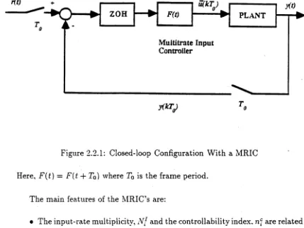
N- (i = 1,2, • • • , m) is term ed the in p u t-rate m ultiplicity. A block diagram showing th e closed-loop configuration with a MRIC is shown in Figure 2.2.1.

2.2. Multirate Input Controllers II

ZOH _PLANT

Multitrate Input Controller

Figure 2.2.1: Closed-loop Configuration With a MRIC

Here. F{t) = F(t -4- T o ) where T0 is the frame period. The main features of the MRIC’s are:

• The input-rate multiplicity. N- and the controllability index, nc{ are related by .V/ > n?.

• They can achieve arbitrary symmetric pole assignment.

• For .V/ > /?.•', they use only gain feedback and are always stable.

• The computational effort in pole assignment is the same as for conven­ tional LTI controllers

12 Chapter 2. Overview of Periodic Controllers

Multirate Sampling

ZOH PLANT

Figure 2.3.1: Closed-loop Configuration with a MROC

Note that the controllers of [16] are a special case of the MRIC’s with N{ = Nj = ■ • • = = N 1 i.e. the controllers of [16] corresponds to a MRIC with uniform input-rate multiplicity. N 1.

2.3

M u ltira te O u tp u t C ontrollers

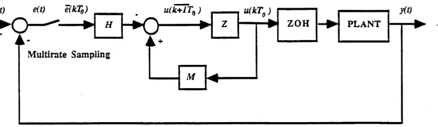
MROC’s are another special class of periodic controllers which employs multi­ rate sampling. Contrary to MRIC's. the sampling mechanism involves detecting the ith plant output at Art° uniformly spaced times and changes the plant input once during one frame period. T0, see [33] for details. A block diagram of the closed-loop configuration with a MROC is shown in Figure 2.3.1.

The main features of the MROC’s are:

• The output-rate multiplicities, N ° and the observability index. n° are related by N ° > n°r

2.3. M ultirate O u tp u t Controllers 13

do not change rapidly.

• For x'VP > n°, the control law uses only output measurements and is equivalent to a state feedback law. As a consequence, observers are not needed in the absence of state measurements.

• For N ° > n°, they can always achieve strong stabilization of an unstable plant i.e. stabilization using an asymptotically stable controller.

• The computational efforts in pole assignment are the same as LTI con­ trollers.

The control law of the MROC’s takes the general form

u{k + 1T0) = Mu(kTo) + He(kT0) (2.3.1)

where M € R mxm, H € R mx* °, N ° = N?, e(t) = r(<) - y(t) and

r ei (fcTo) I

e(kT0) =

e,(fcT0 + N ° - 1 T° )

ep(kT0)

(2.3.2)

[ep(kT0 + N°

which is a collection of the sampled values of the plant output obtained over

[fcTo, (k + l)To) fc = 0,1,2,***.

---th

The above equation means that the control inputs for the fc + 1 frame period are determined based on the values of the control inputs for the kth frame period, u(kT0) and the sampled values of the errors, y{kT0) obtained during the kth frame period. The time available for the computation of u(k + ITq) is evidently rnini<i<pTf>

14 Chapter 2. Overview of Periodic Controllers

CONVENTIONAL PERIODIC CONTROLLER

PLANT

Figure 2.4.1: Conventional Periodic Controller

2 .4

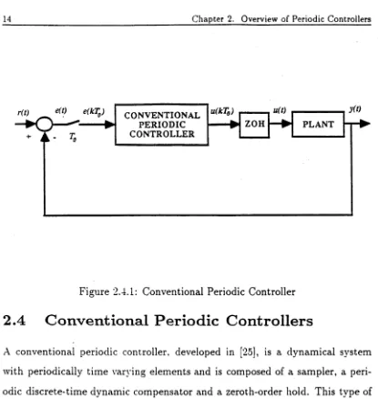
C o n v e n t i o n a l P e r io d ic C o n t r o lle r s

A conventional periodic controller, developed in [25], is a dynamical system with periodically time varying elements and is composed of a sampler, a peri­ odic discrete-time dynamic compensator and a zeroth-order hold. This type of controller is depicted in Figure 2.4.1. Notice the hybrid aspect in this configu­ ration.

A state-space model of this type of controller is given by

£d{k + 1) = + Bd(k)e(kTo) (2.4.1)

u(kT0) = Cd(k)£d{k) + Dd{k)e(kT0) (2.4.2)

where e(t) = r(t) — y(t) and A d(k), Bd( k), Cd(k) and Dd(k) are m-periodic i.e.

Ad{k) = .4,i{k -f m) Bd{k) = Bd(k + m)

2.5. Generalised Sampled-data Hold Function Based Dynamic Compensators 15

The main features of the conventional periodic controllers are:

• Closed-loop zeros can be arbitrarily placed by the controllers.

• Gain margin obtained by the controllers can be significantly improved over that achieved by LTI controllers.

The design procedure consists of

• discretizing the plant.

• designing a LTI dynamic forward-compensator with decimation of the plant output (which is equivalent to the use of a particular form of linear periodic dynamic compensator) to position the zeros of the discretized plant.

• designing a LTI feedback compensator which positions the poles of the discretized plant.

From this procedure, it is not difficult to see that the order of such a con­ troller may be very high due to the introduction of pre-compensation. Another disadvantage, as mentioned in [25], is that the sampling time may have to be very small to permit an increase in the gain margin.

2.5

G e n e r a lise d S a m p le d -d a ta H o ld F u n c tio n

B a s e d D y n a m ic C o m p e n s a to r s

16 Chapter 2. Overview of Periodic Controllers

LTI

CONTROLLER GSHF PLANT

Figure 2.5.1: GSHF Based Dynamic Compensator

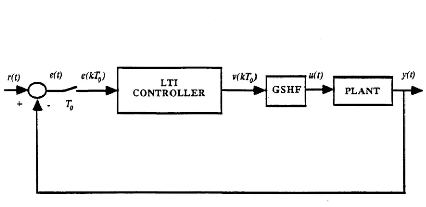
Like a conventional periodic controller, the special feature of a generalised sampled-data hold functions (GSHF) based compensator is the hybrid aspect. The main difference between this configuration and the previous configuration lies in the periodicity; the periodicity of a conventional periodic controller occurs in the dynamic component while the periodicity of a GSHF compensator occurs only in the GSHF gain with the dynamic components time-invariant. The implication of this is that in practice, a GSHF dynamic compensator could be more easily implemented than a conventional periodic digital controller.

A state-space model of a GSHF dynamic compensator is given by

~ d { k + 1) = A cZd(k) + B ce ( k T 0) (2 .5 .1 )

r{k-T0 ) = C c z , i ( k ) + D ce ( kTo) (2 .5 .2 )

u{ t ) = F { t ) v ( k T 0) (2 .5 .3 )

F ( t ) = F ( t + T0 ) (2 .5 .4 )

2.6. GSHF Based Nondynamic Compensator 17

A: = 0 ,1 ,2 ,--*

where e(t) = r(t) — y(t) and T0 > 0 is th e fram e period, / t c, Bc, Cc and Dc are constant m atrices of appropriate dimensions and F ( t ) is a periodic integrable and bounded function m atrix of an appropriate dimension.

T he capability of the GSHF based dynam ic com pensator is sum m arised below:

• For a S1SO, strictly proper, continuous-tim e, FDLTI plant, the closed-loop gain m argin obtained via the com pensator can be significantly improved over th a t achieved via a conventional periodic controller.

• For SISO bicausal and MIMO continuous-tim e FDLTI plants, infinite gain m argin is achieved.

The only drawback of the above controller is th a t for a SISO strictly proper

co n itn u o u s-tim e FDLTI plant, the com pensator so designed is not strictly

causal. T he disadvantages of a nonstrictly causal com pensator are two fold: first, it is well-known th a t it is practically difficult and som etim es impossible to im plem ent a nonstrictly causal com pensator; second, as has been pointed out by [77], stabilisation by a nonstrictly proper com pensator is never robust against singular perturbations.

2.6

G S H F B a s e d N o n d y n a m ic C o m p e n s a to r

The GSHF based nondynam ic com pensator corresponds to the special case of the GSHF based dynam ic com pensator i.e. A c = Bc = Cc — 0, Dc = I in (2.5.1)-(2.5.2), see [38] for details.

18 Chapter 2. Overview of Periodic Controllers

• Simultaneous Pole Assignment: A sufficient condition for simultaneous pole assignability of a finite number of systems by GSHF control is derived.

• Optimal Noise Rejection: A GSHF can be chosen to minimize the sensi­ tivity of the state vector to noise at the sampling times.

• Simultaneuous Optimal Noise Rejection: Optimal noise rejection problem can be solved in a finite number of systems simultaneously by a single GSHF controller.

• Model Matching: A class of closed-loop transfer functions achievable by GSHF control was characterised.

• Decoupling: When decoupling by GSHF is possible and what diagonal closed-loop transfer functions can be achieved were characterised.

• Stability Robustness Analysis: For stable GSHF control loops, pertur­ bations of the open-loop which do not destabilise the closed-loop were characterised.

Note that if the GSHF gain F(t) is implemented on a digital computer by its piecewise constant equivalent, we effectively obtain MRIC’s. (See [79] for details on obtaining a piecewise constant equivalent of F(t)). Therefore, results achievable by MRIC’s as well as the associated drawbacks are applicable to this type of controller.

2 .7

S u m m a r y a n d R e m a r k s

2.7. Summary and Remarks 19

controller in that the GSHF gain is implemented on a digital computer in a piecewise constant manner. In turn, a GSHF based nondynamic compensator is really a special case of its dynamic counterpart.

As we have seen, several interesting results have been accomplished by these five controllers. Given the advantages and disadvantages associated with these controllers, it is natural to ask the following questions:

1. Can one find ways to circumvent their drawbacks ?

2. Can one identify any potential problem associated with the MROC’s al­ though they are the only controllers which do not appear to have any drawback ?

3. Can one possibly employ these controllers or their mechanisms in solving other control problems ?

4. Can one devise other periodic controllers, possibly a mixture of the above, to achieve even more interesting and fruitful control objectives ?

C h a p te r 3

P r a c tic a l Issu e s in M u ltir a te

O u tp u t C o n tr o lle r s

3.1

I n tr o d u c tio n

In this chapter, we seek to identify certain disadvantages of M R O C ’s. We show th a t frame periods and ouput sampling periods must fulfill certain inequality constraints to avoid the gains in the controller becoming very large. Large gains will have the effect of amplifying noise substantially, but not of introducing large controls (in the absence of noise or other non-ideal behaviour). For ease of explanation, the term "frame period” T0 is used to refer to the “cycle” of the controllers and the term "sampling period” is used to indicate the interval in which the plant outputs are detected or inputs are applied; often such sampling periods are multiples or submultiples of 7o.

Section 3.2 reviews the operation of M R O C ’s. Section 3.3 highlights the potential problems via theory and examples and Section 3.4 introduces how these can be avoided through appropriate choice of frame and sampling periods. Section 3.5 contains concluding remarks.

3.2. Review of Operation of MROC’s 21

3 .2

R e v ie w o f O p e r a t io n o f M R O C ’s

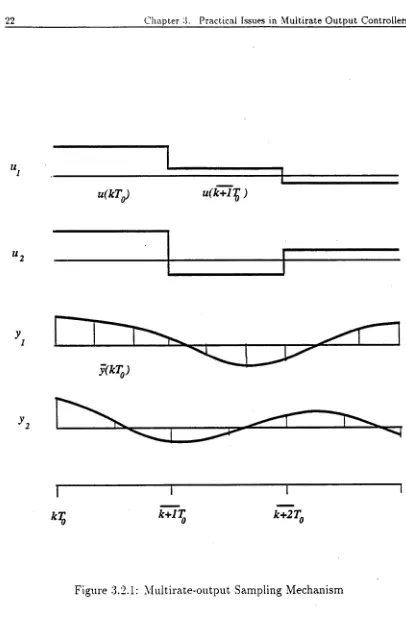
As foreshadowed in the introduction, MROC’s are a special class of periodic controllers which detects the ith plant output at N ° uniformly spaced times and changes the plant input once during one frame period. In order to under­ stand the operation of a MROC, let us first review the concept of multirate output sampling developed in [33]. The MROC’s sampling mechanism involves detecting the 7 t h plant output y, at every T ° seconds where T ° is a submulti­

ple of the so-called frame period 7o as shown in Figure 3.2.1. At time &To, all outputs are sampled and all inputs are changed simultaneously. The sampled values of the plant output obtained over [kTo, (k -j- l)To) are stored in a vector y(kTo) as shown below:

yi{kT0)

y{kTo)

yi(kTo + N ? - 1 T ° )

yP(kT0)

(3.2.1)

L

J

In Figure 3.2.1, N ° = 3 and N ° = 2. The input dimension m as well as the output dimension p is 2.

The vector y(kTo) is used in the control law, which changes the value of u(.) every To seconds. The nature of this control law will now be explained.

Suppose the continuous-time FDLTI plant is described by

x(t) = Ax(t) + Bu(t) (3.2.2)

y(t) = Cx(t) (3.2.3)

where the state x G IRn, the plant input a E IRm and the plant output y E IRP and

22 Chapter Practical Issues in Multirate Out put Controllers

*?

3.2. Review of Operation of M ROC’s 23

We can express the basic formula of the MROC sampling mechanism in a vector- matrix form given by

C x ( k + \ T 0) = y(kTo) - Gu(kTo)

Here, C € IR^ xn and G E xm are respectively given by ' Cle x p ( - A N ° T ° ) '

ci exp( — A T ° )

C = :

cpexP ( ~ A N ? T p°)

. cp exP(—AT°) ,

(3.2.5)

(3.2.6)

G

c\ fo V‘ T{ exp(At)B clt

ci Jo Tl exp( At )Bdt

cp Jo "Vp Tp exp(At)Bdt

cp /o Tp exp(,4£)£? dt

(3.2.7)

where c, is the ith row of C . Equation (3.2.5) gives the relation of the vector y(kTo) for the inputs at the beginning of each frame period and the final state of the frame period.

The integer ;V° is given by

N ° = Y , N ° (3.2.9)

i = i

(The reader is referred to [33] for detailed derivation.)

24 Chapter 3. Practical Issues in Multirate Output Controllers

Definition 3.2.1 Consider an observable pair (A,C) where A E IRnxn and

C E IRpxn. Expressing C as

T l T

then a set of p integers is said to be an observability index vector (abbreviated as OIV) of the pair (A,C) if

p

E » . = (3.2.10)

and

rank[ c'i ■ .4 Vj. ■ • •. • • ,c' A'c’■ ■ ] = n (3.2.11)

Consider the matrix C of the basic formula (3.2.5). In [33], it is proven that the matrix C given b}' (3.2.6) has full column rank (= n) for almost every frame period To if the output-rate multiplicities ( N ° , • • •, N ° ) satisfy

N ° > n°(i = 1,•••,?.) (3.2.14)

where (/?i , • • •, np) is an OIV of the pair (A,C).

A related result, also proved in [33], is the following. Suppose that (A,C) is an observable pair and that

rank ( £ J ) = „ + m (3.2.15)

(which means that p > m, the plant is nondegenerate and the plant has no zero at the origin). Then the matrix [C G] given by (3.2.6) and (3.2.7) has full column rank(= n + in) for almost every frame period Tq if the output-rate multiplicities [Nlf, • • •. ) satisfy

N ° > m, (i = 1, — , p) (3.2.18)

3.2. Review of Operation of MROC's 25

Multirate Sampling PLANT

Figure 3.2.2: Closed-loop Configuration with a MROC

A B

C 0 [C 01

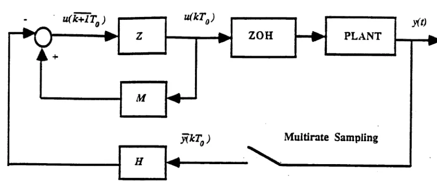
The closecl-loop configuration with a MROC is shown in Figure 3.2.2. The control "law of the MROC takes the general form

u{k + i r 0) = Mu(kTo) - Hy{kT0) (3.2.19) where M 6 IRmx’n and H € IRmx;f0

The above equation means that the control inputs for the k + 1^ frame period are determined based on the values of the control inputs for the kth frame period, u(kT0) and the sampled values of the outputs, y{kT0) obtained during the kth frame period. The time available for the computation of u(k + 1T0) is evidently miri\<i<pT° .

Now. suppose that (.4. C) is an observable pair and the output-rate multi­ plicities ( N ° . • • •, N ° ) satisfy (3.2.14) where (r?i, • • • , n p) is an OIV of the pair (.4.C). Then, if the matrix H can be chosen to satisfy

26 C h a p te r 3. Practical Issues in M ultirate O u t p u t Controllers

and if we set

M = HG (3.2.22)

we can make the control law equivalent to any state feedback control law

u(kT0) = — Fx{kT0) (k > 1) (3.2.23)

This can be argued from (3.2.5) and (3.2.19). Two separate cases can now be considered.

CASE I: Suppose that the output-rate multiplicities (N ° , • • •, N ° ) are set to the minimum values i.e.

N ° = n° {* = (3.2.26)

Then the matrix C becomes a square matrix and H is uniquely determined by

H = FC~ l (3.2.27)

In this case, M is completely determined and this means that the stability of the open-loop controller (which is governed by the eigenvalues of M) depends solely (and indirectly) on the choice of the state feedback matrix F .

CASE II: Suppose that the output-rate multiplicities ( N° , • • •, N ° ) are chosen larger than the minimum values as

i\'P > n" (3.2.28)

3.2. Review of Operation of MROC’s 27

As an approach to achieving this, the authors of [33] proceed as follows. Suppose that (A ,C ) is an observable pair and that

rank ^ ^ ^ ^ = n + m (3.2.30)

Further suppose that the output-rate multiplicities { N ° , • • •, Np ) satisfy

N ° > m t = (3.2.31)

where (m j, • • •, mp) is an 0 1 V of the augmented system.

Then for almost every frame period T0, there exists a matrix H £ IRmx^ such that (3.2.21) and (3.2.22) are both satisfied and where F £ lRmxn is the desired state feedback and M £ IRmxm is an arbitrary specified m?Trix corre­ sponding to the desired state transition matrix of the controller itself. This is because [C G\ has full column rank under the stated assumption, and accord­ ingly, H can be found to satisfy

H[C 6} = [F M] (3.2.32)

(We simply choose H = [F M]E where E is a left inverse of [C G])

The above implies that we can equivalently realize any state feedback F by a MROC possessing any prescribed degree of stability since we can choose the matrix M arbitrarily. The choice M = 0 is of course permissible.

The procedure for strong stabilization of the original plant boils down to choosing a stable feedback matrix F which makes (As — BSF) stable where

As = exp(ATo) (3.2.33)

Bs = [ exp [At) Belt (3.2.34)

Jo

and then choosing a stable matrix M . Finally, it involves determining H by

H = [F M][C G)~L (3.2.35)

28 C h a p te r 3. Practical Issues in M u ltirate O u t p u t Controllers

3 .3

P o t e n t ia l P r o b le m s o f M R O C ’s

In this section, we identify two situations giving rise to potential problems associated with the M RO C ’s. Specifically, we point out two situations for case

I ( A = n°) and for case II ( N ° > n°) where the m atrix C or [C G] can approach a rank deficient matrix. The consequence of this is th a t for almost all desired feedback gains F , the gain m atrix H of the controller will acquire extremely large entries. Although the ideal plant input u ( k T0) will remain well- behaved, taking the value —Fx(kTo), the actual plant input will not, since any inaccuracies in the output, due . for example, to noise or nonlinearity, will be amplified by H.

To fix ideas, assume th at .4 has distinct eigenvalues; then we can always find an invertible m atrix T such th at

A d = T - ' A T (.3.3.1)

to II i Do (3.3.2)

Ci = C T (3.3.3)

with Ad in Jordan form.

For convenience, let us also assume th a t A has real eigenvalues; this keeps the algebra simpler. Further, we arrange Ad such th a t it is given as follows:

Ad A i_{0 a}0 (3.3.4)

where Ad £ IR7lXn, ,4i = clia g (A,). (/' = ! , • • • , (n — 1)) and | a | > | A , | , a £ IR\{0}

B x B

and the A,’s are distinct. Let us also define

3.3. Potential Problems of MROCs 29

w h e r e Bd G H T xm, ß , 6 R |n- ' )x" \ B2 G R lxm a n d

Cd

Cl

C2

. C P .

C \1 C \ 2

C2 i C22

. C pi C p 2 _

w h e re Cd G R px\ ck € R l x n , cM € R lx(n-1) a n d G IR1. T h u s we hav e

C =

ci exp( — T j ° )

ci e x p ( - T dr i° )

cp e x p ( - A dN ° T ° )

(3.3.6)

_ cp — A j T ° ) m

C\i e x p l - Z l i A ^ r P ) c 12 exp(—a N ° T ° )

c n e x p f - A i T j 0 ) c12e x p ( - a T 1° )

cpl exp( - A! A p° T p° ) cp2 exp( - a N °Tp° )

Cp! e x p ( - A i T p° ) cp2 e x p ( - a T p° )

Cu e x p ( - A i T o ) c ]2 e x p ( —a T 0)

cn e x p ( - ^ ) ci2e x p ( - ^ )

Cpi e x p ( - A i T o ) cP2 e x p ( —a T 0)

Cpi ex p( — cp2 e x p ( —^ )

30 C h a p te r 3. Practical Issues in M ultirate O u t p u t Controllers

(Recall that Tf* = -fy)

c\ fo Vl Tl exp{Adt)Bd(lt

c\ fo'Tl exp(Ajt)Bj dt G =

cpfo Np Tp exp{Adt)Bd dt

_ rp O

Cp fo p exp(Adt)Bddt

- ClA ? [ e x p ( - A d N ? T ° ) - I ] B d m

cl A^l [exp{-AdTf) ) - I]Bd

cpA ^ [ e x p ( - A dN?T?) - I]Bd

. cpA j l [ exp{-AdT°) - I]Bd .

Cll Cl 2

. V o '

0 1

Or J

e x p { - A i T 0 ) - I 0

0 e x p ( —qT0 ) — 1

[ Cn Ci2 ' A p 0

0 1

L cv

' e x p ( - ^ ) - 7 0

0 e x p ( - ^ ) - l

Cpl Cp2

a ? o '

0 1

u Or J

e x p ( —A\T0) - I 0

0 e x p ( - a T o ) — 1

’

Ap

a . _.

e x p ( - 4 $ > ) - /

e x p ( - ^ ) - l

3.3. Potential Problems of MROC’s 31

' cnAl ' i expi - AxTo) - I ) B X + ^ ( e x p ( - a T 0) - l ) B2 '

c11A71( e x p ( - ^ S 1) - I)Bi + ^ ( e x p ( - ^ ) - 1 )B2

cplA x l{exp{- Ai T0) - I)B\ + ^ ( e x p( - a T 0) - \ ) B 2

Cp\Ax 1(ex p (-4 j§ i ) — I)B\ + ^ ( e x p ( —^ § ) — 1 )B2

(3.3.8)

3.3 .1 C A S E I:

N ° = n°

In the previous section, we mentioned that when N ° = n°, the state transition matrix M of the controller cannot be freely chosen. In this case, C is square and the design procedure is as follows:

1. Choose the closed-loop poles to be assigned and calculate the state feed­ back matrix F which realizes those poles;

2. Determine H uniquely by

H = FC~ l ; (3.3.9)

3. Determine the state transition matrix M of the controller by

M = HG

= FC~ lG. (3.3.10)

Now, we shall exhibit conditions under which C approaches a singular ma­ trix. Observe first that when To —* 0,

C

C 1 1 C \ 2

C \ \ C \ 2

C p \ C p 2

32 Chapter 3. Practical Issues in Multirate Output Controllers

Evidently, C E and we have Ya=\(N° — 1) rows identical. Now N ° > 1 for at least one i , else we do not have different input and output sampling rates; hence the limiting matrix is again singular.

Next, suppose that a > 0 i.e. the plant is open-loop unstable. (Note that the conclusion above made no assumption concerning stability or instability). As T0 —> oo, the last column of C in (3.3.7) tends to zero and the limiting matrix is again singular.

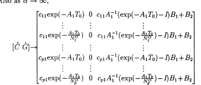
We can also observe that as o —> oc, then

C

cn exp(-AiTo) 0

cu e x p { - 4 ^ ) 0

Cpi exp( Ai Tq) 0

cple x p ( - 4 ^ ) 0 and once again, we see that the limiting matrix is singular.

Let us indicate a subtle point regarding this result. Consider a SISO system, such that

c(s I — A) 16 = n(5) d\(s)(s + tv)

with all coefficients of n($), d\(s) fixed and o variable. Then an easy calculation shows that ||cn|| depends inversely on a and ||c12|| is independent of cr, if 6n, b\ 2 are chosen independently of a. The whole transfer function goes to zero as a —> oo.

If, on the other hand.

c(sl — A) l b = [ni(s) + o n 2(s)] di{s)(s + o)

3.3. Potential Problems of MROC's 33

either case when a —* oo, viz 77.2(3) = 0 or n2(s) nonzero, the conclusion that C

approaches a singular matrix as a —> 00 remains valid, despite the dependence

of Cu, C12 on a. The conclusion obviously also applies to the multivariable case.

3.3.2

C A SE II:

N

?

> n°

For N ° > n°, the state transition matrix M can be freely chosen. The de­ sign procedure is different from the previous case when iV:° = n°. Here, the procedure is as follows:

1. Choose the state transition matrix of the controller M so that it is stable;

2. Choose the closed-loop poles to be assigned and calculate the state feed­ back matrix F which realizes these poles;

3. Determine H bv the following matrix equation

H = [F M][C (3.3.11)

Now, we will study situations where \C G] approaches a matrix with defi- cient column rank. First, when T0 —► 0,

[C G\

C \ \ C \2 0

C u C1 2 0

Cp1 Cp2 0

Cp\ Cp2 b

Obviously, the limiting matrix fails to have full column rank.

34 Chapter 3. Practical Issues in Multirate Output Controllers

[C G'] may tend to infinity or zero or remains finite and nonzero. Thus one can anticipate that a left inverse of the matrix could become unbounded as To —*• oo and this is borne out by a later example.

Also as a —> oo,

c n e x p (-.4 1r 0) 0 C\\AX 1 (exp( — A\Tq) — I)B\ + B2

[C G]

cu e x p { - A ^ ) 0 cu A x +

cpiexp( — A XT0) 0 CpiAj 1( e x p ( - A 1T0) - / ) ß i + ß 2

cpi e x p ( - 4 ^ ) 0 cplA'[l { e x p { - ^ - ) - l ) B l -\-B2 The loss of column rank for the limiting matrix is evident.

(3.3.12)

3 .4

E x a m p le s

To illustrate the above observations, we provide results for some stable and unstable plants in which T0 tends to zero and infinity and a tends to infinity for each of the two cases.

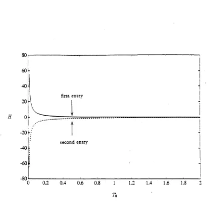
Figure 3.4.1 is for the stable plant

A = - 1 0

0 - 4 4.5

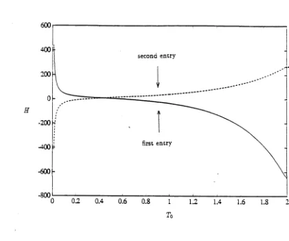
with transfer function given by Since the plant has an observability index of 2, let the output-rate multiplicity be = 2. The graph shows that when T0 tends to zero, entries of the gain vector H blow up. The entries remain finite when T0 becomes large.

Figure 3.4.2 is for the unstable plant

A = 1 0

0 4 3.5

3.4. Examples 35

graph shows that when T0 is too small or too big, entries of the gain vector H blow up.

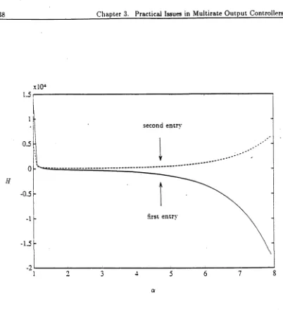
The previous two graphs show the effect of To on stable and unstable plants with fixed a. Figure 3.4.3 shows the effect of varying a with fixed T0 for

A = 1 0 0 a

-0 .5

1 q — 0.5

with transfer function given by • Again, since the plant has an ob­ servability index of 2, we choose the output-rate multiplicity as N ° = 2 for case I. When q is too large, entries of H blow up. The graph also shows that when

a is close to 1, entries of H blow up. This is due to the fact that the plant loses controllability when o = 1 and so pole shifting becomes impossible.

For case II, Figures 3.4.4, 3.4.5 and 3.4.6 illustrate the effect of varying To and q for stable and unstable plants.

Figure 3.4.4 is for

with transfer function given by Since the plant has an observability index of 2, let the output-rate multiplicity be A^0 = 3. The graph shows that when Tq tends to zero, entries of the gain vector H blow up.

Figure 3.4.5 is for

1.5

1 C = 1 4.5

1 0

0 4 3.5

with transfer function given by . Since the plant has an observability index of 2. we take the output-rate multiplicity as A^0 = 3. The graph shows that when T0 tends to zero or a very large value, entries of the gain vector H again blow up.

Figure 3.4.6 is for

.4 = 1 0

0 a B =

-0.5

36 C h a p te r 3. P ra c tic a l Issues in M u ltir a t e O u tp u t C o n tro lle rs

80,

60

H-!

40 K

20 R

Ob

I

-20 i-/

I >'

I; -io H

:

:

-60

K-first entry

second entry

-80

0.6 0.8 1 1.4 1.6

F ig u re 3.4.1: E n trie s o f G ain V e c to r H vs Fram e P erio d T0 fo r

A = - 1 0

3.4. Examples 37

600 r

second entry

first entry

Figure 3.4.2: Entries of Gain Vector H vs Frame Period T0 for

.4

0 4 B =

-0 .5

38 Chapter 3. Practical Issues in Multirate Output Controllers

x l O4

second entry

first entry

Figure 3.4.3: Entries of Gain Vector H vs Largest Mode o for

A = 1 0

0 Q B =

-0 .5 '

3.5. Approaches To Avoid Problems 39

with transfer function given by ■ Take = 3 with observability index of 2. The graph shows that when a tends to a very large value, entries of the gain vector H blow up.

3 .5

A p p r o a c h e s T o A v o id P r o b l e m s

In this section, we indicate some rules of thumb that will ensure that excessive gain values are avoided for case I and case II.

3.5.1

C A SE I:

N ° = n°

E ffect o f To —* 0

Suppose (without loss of generality) that a > |A,|, i = 1,2, • • • , (n — 1). When

exp( — )• // = 1, • • •, (Ar,° — 1) appearing in C in (3.3.7) will also be ap­ proximately 1 i.e. C will be close to singular. Therefore, for proper operation of MROC’s

Note that this gives an upper-bound on the sampling frequency while the sampling theorem gives a lower-bound in that lj0 must be at least two times the closed-loop bandwidth (In practice, a larger multiple value must be assumed).

(3.5.1)

=> cjo < 407TO (rad/s) (3.5.2)

E ffect o f Tq —> oo for a > 0

40 Chapter 3. Practical Issues in Multirate Output Controllers

5000 4000 b 3000 b

2000 b

H 1000 b \

second entry

Ob /

1000b /

-2000 b|

-3000'

third entry

first entry

1.5 15

To

F igure 3.4.4: E n tries of G ain V ector H vs F ram e P eriod T0 for

A = - 1 0

0

- 4 B =

- 1 .5

3.5. Approaches To Avoid Problems 41

x l O4

third entry first entry

second entry

Figure 3.4.5: Entries of Gain Vector H vs Frame Period 7o for

A = 1 0

0 4 B =

-0.5