State-variable and cyclic-averaging analysis of bidirectional CLLC resonant converters

(1)

This is a repository copy of

State-variable and cyclic-averaging analysis of bidirectional

CLLC resonant converters

.

White Rose Research Online URL for this paper:

http://eprints.whiterose.ac.uk/151485/

Version: Published Version

Proceedings Paper:

Lais, M., Stone, D. orcid.org/0000-0002-5770-3917 and Foster, M.P.

orcid.org/0000-0002-8565-0541 (2019) State-variable and cyclic-averaging analysis of

bidirectional CLLC resonant converters. In: IET PEMD 2018. IET PEMD 2018, Liverpool.

IET , Liverpool , pp. 4364-4368.

https://doi.org/10.1049/joe.2018.8072

[email protected]

https://eprints.whiterose.ac.uk/

Reuse

This article is distributed under the terms of the Creative Commons Attribution (CC BY) licence. This licence

allows you to distribute, remix, tweak, and build upon the work, even commercially, as long as you credit the

authors for the original work. More information and the full terms of the licence here:

https://creativecommons.org/licenses/

Takedown

If you consider content in White Rose Research Online to be in breach of UK law, please notify us by

(2)

The Journal of Engineering

The 9th International Conference on Power Electronics, Machines and

Drives (PEMD 2018)

State-variable and cyclic-averaging analysis

of bidirectional CLLC resonant converters

eISSN 2051-3305

Received on 22nd June 2018 Accepted on 31st July 2018 E-First on 30th April 2019 doi: 10.1049/joe.2018.8072 www.ietdl.org

Lais Farias Martins

1

, David A. Stone

1

_{, Martin P. Foster}

1

1_{The University of Sheffield, Department of Electronic & Electrical Engineering, Sheffield S1 4DE, UK}

E-mail: [email protected]

Abstract: The study proposes the application of state variable and cyclic-averaging modelling techniques for analysis of bidirectional, dual active bridge, CLLC resonant converters. The techniques are applied for converters operating under single phase-shift modulation in forward and reverse modes and the equation description is obtained for both models. The design of the converter is presented and the simulation results obtained are compared to a Spice-based simulation to verify the accuracy of the proposed models. Results show the models are suitable to represent the behaviour of CLLC converters under single phase-shift modulation. In addition, when using the cyclic-averaging technique integration is not required to solve the model, which results in a considerably rapid analysis when compared to the execution times of state variable and Spice-based models.

1 Introduction

The interest in electric vehicles (EVs) has been increasing especially due to their reduced CO2 emission levels, government

incentives and increased affordability. Most battery chargers for EVs are unidirectional, allowing power flow only from the grid to the vehicle; however, vehicle-to-grid (V2G) technology requires bidirectional power flow between grid and battery. Consequently, the battery may be available for grid support and to maintain stability at peak times. Typical bidirectional chargers for V2G consist of an AC–DC converter for power factor control and a DC– DC converter for output voltage and current regulation [1].

The dual active bridge (DAB) is a widely used topology of bidirectional DC–DC converter for V2G applications [2–4]. Due to the DAB limitations such as large reactive current, limited operating range and reduced efficiency, resonant variants were proposed to increase efficiency and improve operation for wide input/output voltage ranges [5].

Among various resonant topologies based on the DAB converter, the CLLC converter is a fourth-order resonant topology that provides reduced switching losses, high efficiency and operation under wide voltage range. A considerable advantage of this configuration is the easily achieved soft switching operation for forward and reverse modes when using frequency modulation [6].

To date, most literature focuses on frequency modulated CLLC converters [1, 6, 7]. However, for applications requiring fixed-frequency operation the fixed-frequency modulated control strategy cannot be applied. As an alternative, phase shift modulation can be implemented [8, 9], in this case the phase shift between the bridges or between each leg of the bridges is used to control power flow and direction.

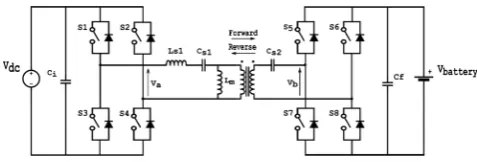
This paper investigates a CLLC bidirectional converter operating under single phase-shift (SPS) modulation, Fig. 1, when only the phase shift between the output voltages of the two active bridges is used to control the output power.

Modelling techniques are employed for converters analysis to facilitate the design process and predict performance. A linear state-variable model using dq transformation for CLLC converters is proposed in [9].

This study proposes two modelling techniques for time-domain analysis of the converter: state variable and cyclic averaging. Here, a simpler non-linear state-variable model is proposed and will serve as base for the implementation of the cyclic-averaging method.

The cyclic-averaging technique was proposed in [10] as an accurate method of time-domain analysis for periodically switched systems. The steady-state values of the state variables are obtained from analytical equations instead of integration. Therefore, steady-state prediction is obtained rapidly when compared with integration-based methods. Previously, cyclic averaging has been used to analyse LLC [11] and inductor-capacitor-capacitor (LCC) converter [12], here then, this is extended to apply cyclic averaging analysis to fourth-order CLLC converters, specifically regarding phase-shift modulated variants.

The paper is structured as follows. In Section 2, the state-variable model is presented. The cyclic-averaging model is described in Section 3. Section 4 contains the converter design and analysis of results.

2 State-variable analysis

Since the converter analysed in this paper is bidirectional, two modes of operation will be studied. In forward mode, the power flows from the DC link, represented in Fig. 1 as the voltage source,

Vdc, to the battery, represented by the source Vbattery. In reverse

mode, the battery serves as a supply to the grid and the power flows from the battery to the DC bus.

2.1 State-variable analysis for forward operation

For the state-variable analysis, the converter from Fig. 1 is divided into two sub-systems [12]. The resonant network is considered the fast system and the output filter constitutes the slow sub-system, with these two sets of state-variable equations being connected by a coupling equation that represents the non-linear behaviour of the output bridge.

The equivalent circuit for state-variable analysis in forward mode is presented in Fig. 2.

[image:2.595.50.289.680.761.2]

(3)

transformer's turns ratio. The resistances of switches and voltage sources are considered to have negligible effect on the voltage generation at the output of each bridge, therefore:

va= ±Vdc (1)

nvb= ±nVbat (2)

Using basic circuit analysis, the state-variable description can be obtained.

The fast sub-system can be described by the following state equations:

diLs1 dt =

va− (r1+r2′)iLs1−vCs1+r2′iLm−vcs2−nvb

Ls1 (3)

dvCs1 dt =

iLs1

Cs1 (4)

diLm dt =

r₂′iLs1− (rLm+r2′)iLm+vCs2′+nvb

Lm (5)

dvCs2′

dt =

i_Ls1−i_Lm

Cs2′ (6)

The slow sub-system is described as

dvCf dt =

Vbat+rbibridge−vCf

Cf(rb+rCf) (7)

The coupling equation is obtained considering the operation of the active bridge on the output side:

i_bridge= n(iLs1−iLm) whenvb> 0 −n(iLs1−iLm) whenvb< 0

(8)

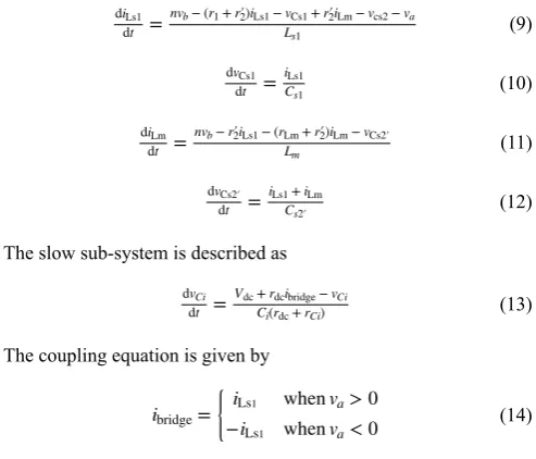
2.2 State-variable analysis for reverse operation

Now considering the opposite power flow direction, the equivalent circuit for reverse mode analysis is shown in Fig. 3 and since the output is now on the primary side both fast and slow sub-systems are referred to the primary.

The fast sub-system can be described by the following equations:

diLs1 dt =

nvb− (r1+r2′)iLs1−vCs1+r2′iLm−vcs2−va

Ls1 (9)

dvCs1 dt =

iLs1

Cs1 (10)

diLm dt =

nvb−r₂′iLs1− (rLm+r₂′)iLm−vCs2′

Lm (11)

dvCs2′

dt =

iLs1+iLm

Cs2′ (12)

The slow sub-system is described as

dvCi dt =

Vdc+rdcibridge−vCi

Ci(rdc+rCi) (13)

The coupling equation is given by

i_bridge= iLs1 whenva> 0 −iLs1 whenva< 0

(14)

3 Cyclic-averaging analysis

Cyclic averaging is a technique used to model periodically switching systems. Due to the switching characteristic of these systems, the state vector does not converge to a fixed value in steady state. Therefore, the steady-state behaviour is obtained by analysing a cycle, and averaging the values of the state variables using the proposed method [10].

The CLLC system presented in this paper is considered cyclic because the state vector at the beginning and at the end of the switching period is equal, therefore:

x(t) =x(t+nT) (15)

where T is the period of the input voltage and n is the number of cycles.

Based on the state of the input voltages va and nvb, each cycle can be divided into operating modes and a state-variable description is obtained for each mode resulting in a set of piecewise linear equations. Each i mode has the following state-variable representation:

x˙₍t) =Aix(t) +Bi (16)

where x˙₍t) is the state vector, A_i is the dynamic matrix and B_i is the

excitation term.

Here, the circuit operates in each mode for a fixed period. The time interval for each mode is given by a duty cycle di. If T is the period of a cycle, the circuit operates in mode i, during di T seconds. For each operation mode, the state vector x˙₍ti) may be

calculated analytically using the following equation:

x˙₍t) = eAi(t−ti− 1)_x₍_t i− 1) +

∫

ti− 1 t

eAi(t−τ)

Bidτ

x˙₍ti) = eAidiTx(ti− 1) +

∫

ti− 1

ti

eAi(ti−τ)

Bidτ

x(ti) =ϕix(ti− 1) + Γi

(17)

where:

ϕ_i=ϕ(ti,ti− 1) = eAidiT, Γi= ∫ti− 1 ti _eAi(ti−τ)_B

idτ= (eAidiT−I)Ai−1Bi if Ai

is invertible.

The calculation of these terms is possible but complex, especially the integral term for cases where Ai is singular. The augment state vector is used to obtain a simplified and rapid solution without the integration. Therefore, the dynamic and input matrices are combined resulting in the following:

d dt

x(t) 1 =

Ai Bi

0 0

x(t)

1 (18)

or

d dtx

^₍_t_{) =}_A^

ix^(t) (19)

The solution for the ith mode is given by Fig. 2 Equivalent circuit for forward mode

Fig. 3 Equivalent circuit for reverse mode

[image:3.595.50.284.180.326.2] [image:3.595.41.288.488.699.2]

(4)

x^(ti) = eA ^_idiT

x^(ti− 1) =ϕ ^

ix^(ti− 1) (20)

Considering a system with m modes, the state vector for mode m, after the whole period is given by

x^(tm) =ϕ ^

mϕ ^

m− 1⋯ϕ ^

1x^(t0) =ϕ ^

totx^(t0) (21)

where x^₍_t

0) is the initial condition.

The matrix ϕ^i can also be obtained from the combination of

matrices ϕi and Γi.

ϕ^_i= ϕi Γi

0 1 (22)

The periodic solution can be found assuming that after a whole cycle the state vector is equal to the initial state, as in (23)

x^_per(t0+T) =ϕ ^

totx^per(t0) =x^per(t0) (23)

where

x^_per(t0) =

xper(t0)

1 (24)

Solving (23) gives

xper(t0) = (In−ϕtot)−1Γtot (25)

where

ϕ_tot=ϕmϕm− 1⋯ϕ1and Γtot= (ϕmϕm− 1⋯ϕ2)Γ1+ (ϕmϕm− 1⋯ϕ3)Γ2

+ ⋯ +ϕ_mΓm− 1+ Γm

Therefore, using (17), (20) and (25) the steady-state value for all state variables can be calculated for any t.

From the cyclic description obtained the average steady-state values of the state variables for a whole cycle can also be calculated. The average value definition is given by

xavg= _T1

∫

t₀

t0 +T

xper(t)dt (26)

Considering the system

x˙₍t) =Aix(t) +Bi

y˙₍t) =x˙_avg₌ 1

Tx(t)

(27)

The augmented state vector method is used again to obtain a simplified solution without integration resulting in

d dt

x(t) 1

xavg(t)

=

Ai Bi 0

0 0 0

I/T 0 0

x(t) 1

xavg(t)

(28)

or

z˙₍t) =A~iz(t) (29)

The averaged state vector can then be obtained calculating z(t0+T)

based on the initial state z(t0). Given the initial state

z(t0) =

x_per(t0)

1 0

(30)

The averaged state vector is then calculated

z(t0+T) =ϕ

~

mϕ

~

m− 1⋯ϕ

~

1z(t0) =

x_per(t0)

1

xav

(31)

where ϕ~i= eA ~

idiT

3.1 Cyclic-averaging analysis for forward operation

Here the cyclic analysis will be shown for forward operation, the same methodology is also applied to the reverse operation.

The state-space description for forward mode previously obtained from (3) to (7) is used as a base for application of the cyclic method. The set of equations can be represented in the matrix form as

d dt

iLs1

vCs1

i_Lm v_Cs2′

vCf

=A

iLs1

vCs1

i_Lm v_Cs2′

vCf

+B (32)

where (see (33)) , and

B=

(va−nvb)

Ls1

0

nvb

Lm

0

V_bat+rbibridge

Cf(rb+rCf

(34)

The state-variable system depends on the state of voltages va and

vb. For a converter operating under SPS modulation there are two possible states for each voltage, leading to four operating modes. The periodic behaviour of the bridge voltages va and vb for forward operation is shown in Fig. 4 and the four modes can be identified for a cycle. When operating in forward mode the right bridge (vb) leads and the power flows from the DC bus to the battery.

At the beginning of the cycle, when the right-bridge voltage vb becomes positive, the four modes are:

A=

−(r1+r2′)

Ls1 −

1

Ls1

rC′2

Ls1 −

1

Ls1 0

1

Cs1 0 0 0 0

rC′2

Lm 0 −

(r_Lm+rC′ )2

Lm

1

Lm 0

1

Cs′2 0 −

1

Cs′2 0 0

0 0 0 0 − 1

Cf(rb+rCf)

(5)

Mode 1: va=−Vdc, vb= Vbat and ibridge= n(iLs1−iLm);

Mode 2: va= Vdc, vb= Vbat and ibridge= n(iLs1−iLm);

Mode 3: va= Vdc, vb=−Vbat and ibridge=−n(iLs1−iLm);

Mode 4: va=−Vdc, vb=−Vbat and ibridge=−n(iLs1−iLm);

Based on each mode description, the substitution of the values on (32) will determine the dynamic matrices Ai and input matrices Bi, where i= 1, 2, 3, 4.

In SPS modulation, the frequency is fixed and the phase shift between the output voltage of the two bridges is a known angle between 0° and 90°. Therefore, the duration of each mode is fixed and can be calculated based on the period value and phase-shift angle. The duty cycle for the first mode is then determined as follows:

d1=₃₆₀PS (35)

The remaining duty cycles are calculated based on the waveforms symmetry: d2= 0.5 −d1, d3=d1 and d4=d2.

Once the state-space description and mode durations are obtained, the cyclic technique is used to model the converter.

From (25), (30) and (31), the steady-state average values of the state variables are calculated and to verify the model over a cycle

(20) and (25) are used to calculate the values of the state variables at the beginning of each mode (at times x0, x1, x2, and x3 in Fig. 4).

4 Results

To verify the models proposed, a converter was designed based on a methodology proposed in [13]. The state variable and cyclic models described in Sections 2 and 3 were simulated in Simulink and MATLAB, validation of the results being done against a component-based Spice simulation.

4.1 Converter design

A 110 W, 48–12 V, CLLC converter is designed to operate at 100 kHz. Considering the DC voltage conversion ratio definition from (36), a conversion ratio close to 1 results in higher efficiency and smaller bridge currents [13]. Therefore, the chosen turns ratio is 4

DCratio=n

V_sec V_pri=n

V_bat

V_dc (36)

where n is the transformer turns ratio.

The resonant network is tuned to the switching frequency as in (37) [13]

ωr2=₍_L 1 s1+Lm)Cs1=

n2 LmCs2= 2

π f_s2 (37)

As a result, a base reactance value Xn can be defined

X_n=X_Cs1−XLs1=XLm=n2XCs2 (38)

The output power can be calculated based on the modulation angle as shown in (39), considering the most significant part of the power is transferred at fundamental frequency.

P_out=8nVdcVbat

n2Xn

sin(ϕ) (39)

where is the modulation angle and max= 90° for SPS

modulation.

The parameters obtained from this design procedure are listed on Table 1.

4.2 Simulation results and model validation

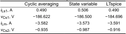
The converter was simulated based on the design developed in the previous section considering forward and reverse operations for three cases of phase-shift angle: 90°, 45° and 22.5°.

The resistance associated to the filter capacitor is neglected and consequently the output voltage is given by the output filter capacitor voltage, vCf for forward mode and vCi for reverse mode. The average value of the output voltage was measured for both models and compared to results from a LTspice simulation. Results for forward operation are shown in Fig. 5 and reverse operation in Fig. 6.

From Figs. 5 and 6, it can be noticed that both state-variable and cyclic-averaging models are accurate compared to Spice. For some points the LTspice result is slightly different, mainly due to the difference in precision used for the average voltage calculation in MATLAB/Simulink simulations (four decimal places) and LTspice simulations (three decimal places).

To verify the accuracy of the models during a whole cycle, the state-variables values on steady state were checked at the beginning of each mode, points x0, x1, x2, and x3 from Figs. 4 and

6. In Tables 2 and 3, the results obtained at point x0 are shown

considering forward and reverse operation.

The results obtained for the two proposed models are similar to the Spice results. Part of the error is a result of the difficulty to measure the current and voltage values for the LTspice and state-variable models at the exact point in time when Mode 1 starts. Fig. 4 Voltages at the output of right (vb) and left bridge (va) for forward

[image:5.595.51.291.49.171.2]

operation

Table 1 Parameter values for CLLC converter

Parameter Value

Vdc 48 V

Vbat 12 V

Cf/Ci 300 F

Ls1 54.04 H

Cs1 31.24 nF

Lm 27.02 H

Cs2 1.5 F

Fig. 5 Average output voltage vs. phase-shift angle – forward mode

[image:5.595.49.285.228.500.2]

(6)

In Table 4, the execution time for the three models is compared. The results obtained by cyclic-averaging method are directly steady state while state variable and Spice models need to be simulated until steady state is reached, around 7 ms for the state-variable simulation and 4 ms for Ltspice. Therefore, for comparison both state variable and spice models have a simulation time of 8 ms with 10 ns step size. The execution time when using cyclic-averaging technique is reduced compared to state variable and Spice models.

5 Conclusions

In this paper, state-variable and cyclic-averaging models were proposed to describe the operation of a bidirectional resonant CLLC converter. The models were developed and simulation results were verified against a Spice simulation. It was shown that both models can be used to accurately predict the behaviour of the CLLC converter and voltage and current stresses on circuit components under phase-shift modulation. Furthermore, it was confirmed that the use of cyclic averaging techniques results in a rapid analysis, with the lowest execution time between the models tested.

6 Acknowledgments

This work has been supported by CNPq – Brazilian National Council of Technological and Scientific Development.

7 References

[1] Sen, B., Liu, C., Wang, J., et al.: ‘A CLLC resonant converter based bidirectional EV charger with maximum efficiency tracking’. 8th IET Int. Conf. on Power Electronics, Machines and Drives (PEMD 2016), Glasgow, UK, 2016, pp. 1–6

[2] Krismer, F., Kolar, J. W.: ‘Efficiency-optimized high-current dual active bridge converter for automotive applications’, IEEE Trans. Ind. Electron., 2012, 59, (7), pp. 2745–2760

[3] Ferreira, R. J., Miranda, L. M., Araújo, R. E., et al.: ‘A new bi-directional charger for vehicle-to-grid integration’. 2nd IEEE PES Int. Conf. and Exhibition on Innovative Smart Grid Technologies, Manchester, UK, 2011, pp. 1–5

[4] Xue, L., Diaz, D., Shen, Z., et al.: ‘Dual active bridge based battery charger for plug-in hybrid electric vehicle with charging current containing low frequency ripple’, IEEE Trans. Power Electron., 2015, 30, (12), pp. 7299– 7307

[5] Gould, C., Colombage, K., Wang, J., et al.: ‘A comparative study of on-board bidirectional chargers for electric vehicles to support vehicle-to-grid power transfer’. IEEE 10th Int. Conf. on Power Electronics and Drive Systems (PEDS), Kitakyushu, Japan, 2013, pp. 639–644

[6] Chen, W., Rong, P., Lu, Z.: ‘Snubberless bidirectional DC–DC converter with new CLLC resonant tank featuring minimized switching loss’, IEEE Trans. Ind. Electron., 2010, 57, (9), pp. 3075–3086

[7] Zahid, Z. U., Dalala, Z. M., Chen, R., et al.: ‘Design of bidirectional DC–DC resonant converter for vehicle-to-grid (V2G) applications’, IEEE Trans. Transp. Electrification, 2015, 1, (3), pp. 232–244

[8] Malan, W. L., Vilathgamuwa, D. M., Walker, G. R., et al.: ‘Novel modulation strategy for a CLC resonant dual active bridge’. 9th Int. Conf. on Power Electronics and ECCE Asia (ICPE-ECCE Asia), Seoul, South Korea, 2015, pp. 759–764

[9] Malan, W. L., Vilathgamuwa, D. M., Walker, G. R.: ‘Modeling and control of a resonant dual active bridge with a tuned CLLC network’, IEEE Trans. Power Electron., 2016, 31, (10), pp. 7297–7310

[10] Visser, H. R., van den Bosch, P. P. J.: ‘Modelling of periodically switching networks’. PESC ‘91 Record 22nd Annual IEEE Power Electronics Specialists Conf., Cambridge, USA, 1991, no. 1, pp. 67–73

[11] Gould, C., Bingham, C. M., Stone, D. A., et al.: ‘CLL resonant converters with output short-circuit protection’. IEE Proc., Electr. Power Appl., 2005,

152, (5), pp. 1296–1306

[12] Foster, M. P., Sewell, H. I., Bingham, C. M., et al.: ‘Cyclic-averaging for high-speed analysis of resonant converters’, IEEE Trans. Power Electron., 2003, 18, (4), pp. 985–993

[13] Twiname, R. P., Thrimawithana, D. J., Madawala, U. K., et al.: ‘A dual-active bridge topology with a tuned CLC network’, IEEE Trans. Power Electron., 2015, 30, (12), pp. 6543–6550

[image:6.595.54.283.49.207.2]

Fig. 6 Average output voltage vs. phase-shift angle – reverse mode

Table 2 Variables at: X for 90° phase shift – forward mode Cyclic averaging State variable LTspice

iLs1, A −3.094 −3.097 −3.136

vCs1, V −3.782 −3.967 −3.880

iLm, A −4.566 −4.567 −4.597

[image:6.595.311.552.224.578.2]

vCs2, V −15.543 −15.510 −15.536

Table 3 Variables at: X for 90° phase shift – reverse mode Cyclic averaging State variable LTspice

iLs1, A 0.490 0.506 0.490

vCs1, V −186.622 −186.500 −184.696

iLm, A −3.582 −3.573 −3.591