City, University of London Institutional Repository
Citation:
Kao, C., Trapani, L. and Urga, G. (2012). Asymptotics for Panel Models with
Common Shocks. Econometric Reviews, 31(4), pp. 390-439. doi:
10.1080/07474938.2011.607991
This is the accepted version of the paper.
This version of the publication may differ from the final published
version.
Permanent repository link:
http://openaccess.city.ac.uk/6113/
Link to published version:
http://dx.doi.org/10.1080/07474938.2011.607991
Copyright and reuse: City Research Online aims to make research
outputs of City, University of London available to a wider audience.
Copyright and Moral Rights remain with the author(s) and/or copyright
holders. URLs from City Research Online may be freely distributed and
linked to.
Asymptotics for Panel Models with Common
Shocks
Chihwa Kao
Syracuse University
[email protected]
Lorenzo Trapani
Cass Business School
[email protected]
Giovanni Urga
Cass Business School and Universita’di Bergamo
[email protected]
July 30, 2010
Abstract
This paper develops a novel asymptotic theory for panel models with common shocks. We assume that contemporaneous correlation can be generated by both the presence of common regressors among units and weak spatial dependence among the error terms. Several characteristics of the panel are considered: cross-sectional and time-series dimensions can either be …xed or large; factors can either be observable or unobserv-able; the factor model can describe either a cointegration relationship or a spurious regression, and we also consider the stationary case. We derive the rate of convergence and the limit distributions for the ordinary least squares (OLS) estimates of the model parameters under all the aforemen-tioned cases.
JEL Classi…cation: C13, C23.
Keywords: Panel data, common shocks, cross-sectional dependence,
asymptotics, joint limit, martingale di¤erence sequence.
1
Introduction
There is a growing body of literature dealing with limit theory for nonstationary panels. While the …rst generation of these contributions assumed independence across units (see for instance Phillips and Moon, 1999; Kao, 1999), in the second generation this assumption is relaxed, and hypothesis testing and estimation methods are evaluated assuming various degrees of cross-sectional dependence, e.g., see Bai (2003, 2004), Bai and Ng (2002, 2004), Stock and Watson (2002). We can distinguish the case where regressors are cross-sectionally dependent (see Donald and Lang, 2004; Moulton, 1990) from the case where it is the error terms across unit to be dependent (see for instance Bai and Kao, 2006; Moon and Perron, 2004) or both (see for instance Ahn, Lee, and Schmidt, 2001; Pesaran 2006).
The main aim of this paper is to propose a novel asymptotic theory for panel models where common shocks are present among the regressors, thereby introducing strong cross-sectional dependence. We generalize the asymptotics developed by Phillips and Moon (1999) and Andrews (2005) by employing and extending the theory for factor models in Bai (2003, 2004) and Bai and Ng (2004).
asymptotic normality, as Andrews (2005) has demonstrated in a cross-sectional context. Andrews (2005, Theorem 4, p. 1567) proves that the presence of com-mon factors acom-mong the cross-sectional units makes the limiting distribution of the OLS estimator of the regression slope mixed normal and not normal as in the classical regression analysis. Note that in this case mixed normality of the OLS estimator of the regression slope holds even if regressors are stationary, i.e.,I(0);and independent of errors. This …nding is also obtained in our paper when studying the distribution limit for the OLS estimator of the regression slope for the …xedT case (see equation 20 in Theorem 2 below), while when we consider theT ! 1case, not explored by Andrews (2005), we show that in the stationary case asT ! 1the OLS estimator of the regression slope is normally distributed.
1.1
Basic Model and Extensions
In this paper we consider the following panel regression model with common shocks
yit= i+ 0Ft+uit (1)
i= 1; :::; n; t= 1; :::; T, where is a k 1 vector of slope parameters and the regressorFt= (F1t; :::; Fkt)0 is ak 1vector of common shocks,
Ft=Ft 1+"t:
Equation (1) could be either a spurious regression or a cointegration model de-pending on whetheruitisI(1)orI(0), respectively. It is important to emphasize
that, as far as the presence ofFt is concerned, equation (1) represents a panel
regression model with a set of regressors,Ft, which is common across units and
with common slope coe¢ cient . Model (1) di¤ers from a factor-loading speci…-cation as in Bai (2004) and Bai and Ng (2004), for example. Thus, in our setup
Ft is a genuine (observable or unobservable) regressor rather than a “common
factor”. A framework which is similar in spirit to the one in this paper is in Stock and Watson (1999, 2002, 2005), whereyitin (1) (withn= 1) is the
multiple time-series of candidate predictors; also, model (1) resembles the panel cointegration model with global stochastic trends of Bai, Kao and Ng (2009), although (1) assumes having common .
When common shocks are not observable, we assume that a set of exogenous variables,zit, is observable such that
zit= 0iFt+eit (2)
where i is a vector of factor loadings and eit is an idiosyncratic component.
We assume throughout the paper, for the sake of the simplicity of the notation, that the number of thezits is the same as that of theyits. However, the panel
dimensions of yit and the zit may be di¤erent, for example yit may refer to
individuals whilezitmay index several macro variables.
To extend our results to the stationary panel model case, we also consider the …rst-di¤erenced form of model (1),
yit= 0 Ft+ uit: (3)
Model (1) considers a very simple speci…cation. However, it could be ar-gued that a more complete and realistic framework should also embed a set of idiosyncratic shocks, i.e.,
yit= i+ 0Ft+ 0xit+uit: (4)
For the sake of notational simplicity, the main results in the paper, reported in Section 3, are derived under the restrictive assumptions of no idiosyncratic shocks, i.e., under the constrain that = 0. However, in Section 4 we show that our main results concerning the asymptotics of the estimator of are still useful in presence of a more complicated speci…cation as (4). This is obviously true when the regressorsFt andxit are orthogonal. We also examine the case
whereby the xit are allowed to be correlated with Ft via the factor-loadings
speci…cation
whereGtis a set of common factors that can be independent of the regressors
Ft or (fully or partly) overlap with them, and!it is a unit speci…c (stationary
or nonstationary) shock. A similar framework that allows for cross-sectional dependence among the idiosyncratic regressors and dependence between the idiosyncratic regressors and the common regressors is in Pesaran (2006) and Kapetanios, Pesaran and Yamagata (2006), even though in our paper Ft is a
set of regressors and not nuisance parameters. Note that allowing forxitbeing
dependent uponFtthrough some possibly heterogeneous loadings i allows for
the response ofyit toFt being (indirectly) heterogeneous across individuals.
Models (1) and (4) are frequently employed for the purpose of forecasting (Stock and Watson, 1999, 2002, 2005), and they encompass a wide set of models in economics and …nance. As a general interpretation, such models represent the decision of a microeconomic agent i (yit), being in‡uenced by macroeconomic
factors Ft and by a set of individual speci…c characteristics, i and possibly
xit. Examples in the literature include, inter alia: demand for household food
consumption (see e.g., Dynarski and She¤rin, 1985, where households are as-sumed to have the same elasticity to food price, which is the common shock, and to permanent income, which is the idiosyncratic variable); …rm size evolv-ing accordevolv-ing to a random walk, a case known in the literature as Gibrat’s law (see Sutton, 1997; Geroski et al., 2002); other examples can also be found in micro demand for investment, consumption, labor demand. Moreover, the forward rate unbiasedness hypothesis postulates that the forward rate is an un-biased predictor of the corresponding future spot rate. This hypothesis has been extensively tested for exchange rates (Baillie and Bollerslev, 1989; Liu and Maynard, 2005; Westerlund, 2007). Another example in …nance are models for default intensity for …rmi at time t expressed as function of common factors (such as U.S. 3-month T-bill and the trailing 1-year returns) and idiosyncratic covariates such as distance to default and trailing 1-year stock return of the …rm
degrees of access to the technological knowledge (Pesaran, 2007; Phillips and Sul, 2007). Considering (3), which represents a stationary panel regression with common shocks, the most natural application one may have in mind is to asset pricing models, such as the APT, where asset returns are explained by common factors (such as e.g., market return and powers thereof to represent coskewness and cokurtosis, macro factors, etc.); see Cochrane (2005) for a comprehensive review.
1.2
Main Results
Our asymptotic theory considers several features of the underlying model. First, we assume that contemporaneous correlation can be generated by both the presence of common regressors (e.g., macro shocks, aggregate …scal and mone-tary policies) among units and weak spatial dependence among the error terms. Second, the common shocks can either be known or unobservable. Classical examples of observed common shocks are index models such as those used in in-ternational trade, labor economics, urban regional, public economics and …nance literature. Most often, shocks are unknown, as in the cases of index extraction and indicators aggregation in economics, e.g., Quah and Sargent (1993), Forni and Reichlin (1998), and Bernanke and Boivin (2000). Third, regression model (1) may describe either a cointegration relationship or a spurious regression. Fourth, the time-series dimensionT and the cross-sectional dimensionncan be either …xed or large. We develop our limit theory by considering cases where the time-series dimension T and the number of units n are large and we also include the case of when eithernorTis …xed.
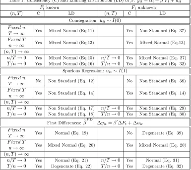
An overview of the results derived in this paper is reported in Table 1.
[Insert Table 1 somewhere here]
As Table 1 shows, this paper provides a uni…ed framework for the asymp-totics of panels with common shocks. Particularly, results for the case of large
Table 1: Consistency (C) and Limiting Distribution (LD) of^: yit= i+ 0Ft+uit
Ftknown Ftunknown
(n; T) C LD (n; T) C LD
Cointegration: uit I(0)
F ixed n
T ! 1 Yes Mixed Normal (Eq.11) Yes Non Standard (Eq. 37) F ixed T
n! 1 Yes Mixed Normal (Eq.13) Yes Mixed Normal (Eq.13)
(n; T)! 1
n=T !0 Yes Mixed Normal (Eq.15) n=T !0 Yes Mixed Normal (Eq. 27) T =n!0 Yes Mixed Normal (Eq.16) T =n!0 Yes Non Standard (Eq. 32)
Spurious Regression: uit I(1)
F ixed n
T ! 1 No Non Standard (Eq. 12) No Non Standard (Eq. 38) F ixed T
n! 1 Yes Non Standard (Eq. 14) Yes Non Standard (Eq. 14)
(n; T)! 1
n=T !0 Yes Non Standard (Eq. 17) n=T !0 Yes Non Standard (Eq. 29) T =n!0 Yes Non Standard (Eq. 18) T =n!0 Yes Non Standard (Eq. 30)
First Di¤erences: ^F D: yit= 0 Ft+ uit
F ixed n
T ! 1 Yes Normal (Eq. 19) No Degenerate (Eq. 39) F ixed T
n! 1 Yes Mixed Normal (Eq. 20) Yes Mixed Normal (Eq. 20)
(n; T)! 1
of the asymptotic theory for panels derived by Phillips and Moon (1999) and Kao (1999), who consider a model with cross-sectional independence. Assum-ing cross-sectional dependence in the panel changes the asymptotic theory, and a typical feature (discussed in greater details hereafter) is the asymptotic dis-tribution of estimates being no longer normal as opposed to the independence case. An important result here is the extension of the joint limit theory to the strong dependence case, and the development of a method of proof for the as-ymptotics of double sums involving common shocks. Thus, although our results are speci…c to model (1), the method of proof we follow can be extended to study the asymptotics of estimators and tests for di¤erent models. For exam-ple, the method of proof developed here extends readily to inferential theory for cointegrated panels with common factors (Westerlund, 2007) or it can be used to show the asymptotics of t-tests for long run parameters in mixed panels (Fuertes, 2008; Ng, 2008); other applications to models where common factors are treated either as nuisance parameters or are genuine observable regressors are possible.
Results obtained for the case whereby the common shocks Ft are not
ob-servable are also new. The asymptotic theory for the estimates of the common shocksFtis based on previous work by Bai (2003, 2004) and Bai and Ng (2002,
2004), and extended to the case of …niten. When common shocks are not ob-servable, the estimated latent variablesFt are used as generated regressors to
estimate . This introduces a new error component in the regression equation. An important contribution of our paper is to study the impact of the estimation error when one needs to use an estimate ofFtin the regression model; see e.g.,
although in a nonparametric set-up, Connor, Hagmann and Linton (2007). Note that in Table 1, the “non standard” limiting distributions depend also on the assumptions made on the data generating process (DGP). Section 3 provides details on this.
T, n=T ! 0. Although more details on the method of proof are provided in Theorem 9 in Appendix B and in the remarks and proofs (reported in Appendix C) of the other theorems, the derivation of the joint limit is carried out by conditioning on the -…eld generated by the common shocksFt. We show, in a
similar spirit to Andrews (2005), that this entails that the quantities involved in the derivation of the asymptotics are martingale di¤erence sequences (MDS), conditional onFt. For each of the cases considered here, we then prove a joint
Liapunov condition, under(n; T)! 1, which allows to apply the MDS central limit theorem (CLT) discussed in Hall and Heyde (1980) as (n; T)! 1. The restriction on the rate of expansionn=T is derived using similar arguments as in Phillips and Moon (1999), based on the Beveridge-Nelson (BN) decomposition of the series involved in the calculations.
The remainder of the paper is organized as follows. Section 2 introduces and comments on the main assumptions. In Section 3, we report the asymptotic the-ory of the ordinary least square (OLS) estimators of in models (1) and (3). We analyze both the cases of known factors (Section 3.1) and unknown factors (Sec-tion 3.2), and we distinguish the cases of largenandT, …niteT and largenand …nitenand largeT. Section 4 considers a discussion of the asymptotics for the estimator of when the data are generated by (4). Some Monte Carlo evidence is reported in Section 5. Section 6 concludes. Appendix A reports and discusses a joint MDS CLT. The main proofs are reported in Appendix B, contained in the present paper. Other proofs and preliminary Lemmas are in Appendix C in an extended, working paper version of this paper, which can be found at
http://www.cass.city.ac.uk/cea/research_papers/WorkingPapers2010/WP_CEA_01_2010.pdf
Notation is fairly standard. Throughout the paper, kAk denotesptr(A0A),
!the ordinary limit,)weak convergence, and!p convergence in probability. Stochastic processes such asB(r)on [0;1] are usually written as B, integrals such as R01B(r)dr as RB and stochastic integrals such as R01B(r)dB(r) as
R
2
Model and Assumptions
We assume thatyitis generated as follows
yit = i+ 0Ft+uit
Ft = Ft 1+"t (6)
zit = 0iFt+eit
i= 1; :::; n;t= 1; :::; T; is ak 1vector of slope parameters;Ft= (F1t; :::; Fkt)0
is ak 1vector of common shocks;uitmay beI(1)orI(0)(spurious regression
or cointegration relationship);zit is a set of observed exogenous variables.
De…neB"as the Brownian motion associated with the partial sums of"twith
covariance matrix "" andB"(r)as the demeaned Brownian motion associated
to the partial sums ofFt, i.e.,B"(r) =B"(r)
R1
0 B"(r)dr. The following set
of assumptions are used throughout the paper:
Assumption 1: (a) Either (i) (cointegration case) uit = Di(L) it, or (ii)
(spurious regression case) uit = Fi(L) it with Fi(1) 6= 0 and such that
P
iuit I(1); for both cases, it i:i:d:
0; 2 overt andi, withEj
itj
8
< M,
P1
j=0jjDijj< M, P1j=0jjFijj< M andD2i (1) 2 >0,Fi2(1) 2 >0; the two
MA processesuit=Di(L) it and uit=Fi(L) it are assumed to be
invert-ible; (b) (time-series and cross-sectional correlation) lettingE(uitujs) = ij;ts= ij;jt sjandE( uit ujs) = ij;ts= ij;jt sj, asn! 1a law of large numbers
(LLN) and a CLT hold for the quantitiesn 1=2P
iuit andn 1=2Pi uit.
Assumption 2: "t =C(L)wt where C(L) =P1j=0CjLj; (a) wt i:i:d:
(0; u)
withEkwtk4+ M for some >0; (b)V ar( Ft) = F =P1j=0Cj uCj0 is
a positive de…nite matrix; (c)P1j=0jkCjk< M and (d)C(1)has full rank.
Assumption 3: EkF0k4 M andEjui0j4 M.
Assumption 4: The loadings i are non random quantities such that (a)
, ifn! 1; in both cases, the matrix is positive de…nite and such that the eigenvalues of the matrix 1=2 F 1=2are distinct, and the eigenvalues of
the stochastic matrix 1=2R B"B0"
1=2
are distinct with probability 1.
Assumption 5: eit = Gi(L) it where (a) it i:i:d:
0; 2
vi , Ejvitj8 < M,
P1
j=0jjGijj < M and G2i(1) 2vi > 0; (b) E( it jt) = ij with Pni=1j ijj
M for all j; (c)E n 1=2Pn
i=1[eiseit E(eiseit)] 4
M for every (t; s); (d)
E n 1Pn
i=1eiteis = s t, s t M for allsandT 1
PT s=1
PT t=1 s t
M; (e)Ejei0j4 M.
Assumption 6: f"tg, fuitg and feitg are three independent groups; F0 is
independent offuitgandfeitg.
Assumption 1(a) considers the possibility that equation (1) is either a coin-tegration or a spurious regression. Processes uit and uit are assumed to be
invertible MA processes as in Bai (2004) and Bai and Ng (2004), in a similar fashion to processes "t and eit. Assumption 1(b) also considers the presence
of some, limited, cross-sectional dependence among the uits or the uits and
therefore it rules out the possibility that all the cross-sectional dependence is taken into account by the common factors Ft, e.g., see the related work by
Conley (1999).
Even if it refers to a di¤erent framework (panel data with common shocks as opposed to factor models), we take a position similar to that in Bai (2003, 2004) and Bai and Ng (2002, 2004). Using the factor models terminology, this means having a model with an “approximate factor structure”, which di¤ers from a strict common factor model where theuitare assumed to be independent across
i, e.g., Chamberlain and Rothschild (1983) and Onatski (2005).
The amount of cross-sectional dependence we allow for in Assumption 1(b) is anyway limited, since we require that it allows a LLN and a CLT to hold for the (rescaled) sequencesPni=1uit andPni=1 uit.
Assumption 2 allows for some weak serial correlation in the dynamics of
absolute summability conditions. Both the short run and the long run variance of Ft are positive de…nite (Assumptions 2(b) and 2(d), respectively). Note
that Assumption 2(d) rules out the possibility that the (common) regressorsFt
in model (1) are cointegrated. This requirement is standard in cointegration to have non-degenerate limiting distributions.
Assumption 3 is a standard initial condition requirement. Assumption 4 serves to identify the factor loadings, which, merely for the purpose of a concise discussion, are assumed to be non random. This requirement could be relaxed, as in Bai (2003, 2004) and Bai and Ng (2004), assuming that the iare randomly
generated and independent of"t and eit, and our results would keep holding.
Assumption 4(b) ensures that the factor structure is identi…able. Note that it would be possible to relax this assumption by constraining the minimum eigenvalue ofPni=1 i 0ito tend to in…nity asn! 1, as pointed out by Onatski
(2005). This structure would allow factors to be less pervasive than in our framework, thereby allowing the idiosyncratic component eit in equation (2)
to have a greater impact in explaining the contemporaneous correlation among thezit. Nonetheless, this would be made at the price of losing the possibility
to model thezit as a serially correlated process, whilst in our framework some
limited time-series and cross-sectional dependence in model (2) is allowed for as one could realize from Assumption 5. As pointed out in Bai (2003), the conditions in Assumption 5 are fairly general and allow for consistency and distribution results to hold for the principal component analysis (PCA).
Assumption 6 also rules out the existence of any form of dependence between factorsFtanduit. Therefore, it is a stronger requirement than the simple lack
of correlation, and we need it in order to prove the main results in our paper. The following de…nitions are employed throughout the paper. Let hi (hi )
andhij (hij) be the long run variance foruit( uit) and the long run covariance
between processesuitandujt( uitand ujt) - we havehij = limT!1T 1PTt=1
PT s=1 ij;ts
andhij= limT!1T 1PTt=1
PT
s=1 ij;ts. Also, leth= limn!1n 1Pni=1
Pn j=1hij
and h = limn!1n 1Pni=1
Pn
j=1hij. Last, the following variances arising
re-sults: ts= limn!1n 1Pni=1
Pn
j=1 ij;ts, and ts= limn!1n 1Pni=1
Pn
j=1 ij;ts.
3
Asymptotic Theory
The main objective of this paper is to derive the rate of convergence and limiting distribution of the OLS,^
^ =
" n X
i=1
T
X
t=1
Ft F Ft F 0
# 1 n
X
i=1
T
X
t=1
Ft F yit (7)
in equation (1), whereF=T 1PTt=1Ft, and ^ F D
when using equation (3),
^F D=
" n X
i=1
T
X
t=1
Ft Ft0
# 1" n
X
i=1
T
X
t=1
Ft yit
#
: (8)
We consider several features of (1) and (3):
1. the shocksFt can either be known or (more likely) unobservable;
2. the relationship described by equation (1) can be either a cointegration relationship or a spurious regression. As pointed out by Kao (1999) and Phillips and Moon (1999), convergence is obtained at rate pn in panel spurious regression models andpnT for panel cointegrated models;
3. the time series dimension T and the cross-sectional dimensionn can be either …xed or large.
We …rst start with the exploration of the case of known common shocks (Section 3.1) and then move to the case of unknown common shocks (Section 3.2).
3.1
Observable
F
tWhenFtis known we have:
^ =
" n X
i=1
T
X
t=1
WtWt0
# 1" n
X
i=1
T
X
t=1
Wtuit
#
whereWt=Ft F, and
^F D =
" n X i=1 T X t=1
Ft Ft0
# 1" n
X
i=1
T
X
t=1
Ft uit
#
: (10)
The convergence rate and the limiting distribution for ^ are stated in the following theorem.
Theorem 1 Suppose Assumptions 1-6 hold, and de…neZ N(0; Ik),
indepen-dent of theFts. For …xednandT ! 1
T ^ ) 1 n
Z
B"B0"
1=20
@ n X i=1 n X j=1 hij 1 A
1=2
Z; (11)
if equation (1) is a cointegration relationship, and
^ ) Z B
"B"0
1 Z
B"Bu
0 @ n X i=1 n X j=1 hij 1 A
1=2
; (12)
if (1) is a spurious regression. For …xedT andn! 1, we have
p
n ^ )
T
X
t=1
WtWt0
! 1 T
X
t=1
T
X
s=1
WtWs ts0
!1=2
Z; (13)
if (1) is a cointegration regression, whilst if it is a spurious relationship we have
p
n ^ )
T
X
t=1
WtWt0
! 1 T
X
t=1
Wtut
!
; (14)
whereut= limn!1n 1=2Pni=1uit.
Let equation (1) be a cointegration relationship; as(n; T)! 1with n=T !0:
p
nT ^ )
"p
h
Z
B"B"0
1=2#
Z; (15)
as(n; T)! 1with T =n!0:
T3=2 ^ )
Z
B"B0"
1
1; (16)
where 1 is de…ned in the proof - see equation (61).
Let equation (1) be a spurious regression; as(n; T)! 1 withn=T !0:
p
n ^ )
Z
B"B0"
1 Z
B"Bu
p
as(n; T)! 1with T =n!0:
p
T ^ )
Z
B"B"0
1
2; (18)
where 2 is de…ned in the proof - see equation (64).
Proof. See Appendix B.
Equation (12) is a standard results in the literature. With respect to the speed of convergence, when (n; T) ! 1 our results lead to the same rates of convergence as in Phillips and Moon (1999) and Kao (1999) for both the cointegration and the spurious regression case. Consistency is achieved under the spurious regression case as well, where the rate of convergence ispn. Note that, irrespective of model (1) being a cointegration regression or a spurious regression, largenallows for consistency to hold.
For the case of (n; T) ! 1 with n=T ! 0, the rate of convergence for ^ is the same as in Phillips and Moon (1999) under the case of contemporaneous independence across cross-sectional units. The limiting distributions in (15) and (17) are mixed normal rather than normal, as in Phillips and Moon (1999). The mixed normality is due to bothFtbeing nonstationary and common across
cross-sectional units, as can be seen by considering equation (13) forT ! 1. The design matrix nT2 1Pn
i=1
PT
t=1FtFt0 =T 2
PT
t=1FtFt0 converge in
dis-tribution to a random matrix, namelyR B"B"0, rather than to a constant. Of
course, nT2 1Pni=1PTt=1FtFt0 would converge to a constant (in probability)
ifFt were not common shocks, i.e., ifFt were replaced byFit. Theorem 1 also
explores the case of a “short”panel, whereT =n!0. In this case, ^ is still con-sistent, irrespective of whether (1) is a cointegration or a spurious regression, although consistency is achieved at a “slower” rate than in the case whereby
n=T !0. The limiting distributions, given in (16) and (18), are non standard, and they depend upon 1and 2. As shown in Appendix C, these terms come
from the bias arising from the BN decomposition ofFt anduit, and thus they
depend upon the assumptions on the DGP ofFtanduit. A similar argument is
set equal to zero, and if they were i.i.d. processes, then (15) and (17) would hold for(n; T)! 1for all combinations ofnand T.
The convergence rates and the limiting distributions for ^F D are reported in the following theorem.
Theorem 2 Suppose Assumptions 1-6 hold and de…neZ N(0; Ik),
indepen-dent of the Fts.
For …xednandT ! 1
p
T ^F D )n 1 1F=2
0 @
n
X
i=1
n
X
j=1
hij
1 A
1=2
Z: (19)
ForT …xed andn! 1, we have
p
n ^F D )
T
X
t=1
Ft Ft0
! 1 T
X
t=1
T
X
s=1
Ft Fs ts0
!1=2
Z: (20)
When(n; T)! 1, under n=T !0 it holds that
p
nT ^F D ) 1F=2ph Z; (21)
as(n; T)! 1, underT =n!0, it holds that
T ^F D !p 1F 3; (22)
where 3 is de…ned in the proof - see equation (??).
Proof. See Appendix C.
Since the …rst di¤erenced model is always stationary, irrespective of whether equation (1) is a cointegration equation or a spurious regression, one can always apply the CLT to obtain the limiting distribution of ^F D .
Equation (21) states that the limiting distribution of ^F D is normal instead of mixed normal, despite the strong dependence across cross-sectional units. This can be seen from equation (20), which gives the limiting distribution forT …xed andn! 1. The matrixT 1PtT=1 Ft Ft0 is random for …niteT,
Equation (22) refers to a panel where T =n ! 0, and thus the number of cross-sectional units is “much larger” than the number of time-series observa-tions. This case is similar to that found in Theorem 1: when T =n ! 0, the bias in the BN decomposition dominates, thereby making the limiting distribu-tion non standard and depending upon the assumpdistribu-tions on the DGP ofFtand
uit. Of course, if one knows 1F 3(or could estimate it consistently at a rate
nT) then the remainder in the BN decomposition of ^ F D
+ 1F 3 has
mean zero (or of order Op( nT)). Under additional assumptions, the bias in
the BN decomposition for 1FPni=1PtT=1 Ft uit (see also equation (??) in
Appendix C) is of orderOp(pn)(resp.,Op(n nT)). Therefore, when
normal-ized by pnT, the bias is always dominated by the martingale approximation to 1FPni=1PTt=1 Ft uit - resp., of order Op pnT nT . The former case
implies that (21) holds as (n; T) ! 1, with no restriction on the rate of ex-pansion ofnandT as they pass to in…nity. This is consistent with Phillips and Moon (1999, p. 1074, Remark (a)), and a similar argument could be in principle applied to Theorem 1.
3.2
Unobservable
F
tWe turn now to the case when common shocks are unknown and thus they need to be estimated. The asymptotics of ^ and ^F D are a¤ected by the errors in estimating shocksFt.
LetF^tbe an estimate ofFt. DenoteW^t= ^Ft T 1PTt=1F^t. Estimation of
using the model in levels or …rst di¤erences respectively are now given by:
^ =
" n X
i=1
T
X
t=1
^
WtW^t0
# 1" n
X
i=1
T
X
t=1
^
Wtyit
#
(23)
and
^F D=
" n X
i=1
T
X
t=1
^
Ft F^t0
# 1" n
X
i=1
T
X
t=1
^
Ft yit
#
(24)
with estimation errors:
^ =
" n X
i=1
T
X
t=1
^
WtW^t0
# 1( n
X
i=1
T
X
t=1
^
Wt Wt W^t
0
+uit
)
and
^F D =
" n X
i=1
T
X
t=1
^
Ft F^t0
# 1( n
X
i=1
T
X
t=1
^
Ft Ft F^t
0
+ uit
)
:
(26)
We assume that the number of common shocksk is known. This does not lead to any loss of generality since the distribution of the estimated shocks does not depend on whether kis known or estimated, and therefore the estimation error that arises from usingk^instead ofkdoes not play any role as long ask^is consistent, e.g., see Bai (2003, p. 143, note 5).
3.2.1 The case of n and T large
In this section, we estimate the common shocksFtusing the principal component
estimator. This means minimizing either
Vb(k) =
1
nT
n
X
i=1
T
X
t=1
zit 0iFt
2
when consideringFt in levels, or
Va(k) =
1
nT
n
X
i=1
T
X
t=1
zit 0i Ft
2
when estimating shocks Ftfrom (2). Consider theT nmatrixZ= (z1; :::; zT)0,
and theT kmatrix of shocksF = (F1; F2; :::; FT)0. Then each objective
func-tion Va(k) or Vb(k) can be minimized by concentrating out and obtaining
estimates F^ andF^using the normalizations F^0 F =T^ =IkorF^0F =T^ 2=I
k.
The estimated shock matrices F^ andF^ arepT andT times respectively the eigenvectors corresponding to the k largest eigenvalues of the T T matrices
Z Z0 or ZZ0.
In the context of unobservable common factors, the problem of identi…cation arises. It is well known (see e.g., Bai, 2003, and Bai, 2004) that the solutions to the above minimization problems are not unique, e.g., when estimating shocks
Ft and Ft, these are not directly identi…able even though they are up to a
the space spanned by the common factors FtandFt, it is not possible to
esti-mate FtandFtthemselves. Thus,F^tand F^tare, respectively, “consistent”
estimators forH0
1FtandH10 Ft, whereH1is a non singulark kmatrix,
mean-ing thatF^t H10Ftand F^t H10 Ftconverge to zero in some sense. This makes
it impossible to estimate consistently, although once again the space spanned by can be estimated consistently. Due to the rotational indeterminacy of the estimation ofFt and Ft, the estimators ^ and ^
F D
may “consistently” esti-mateH11 , so that ^ H11 may converge to zero in some sense asnandT
(or either) pass to in…nity. Whilst there is no direct consistency result for , being able to estimate the space it spans is su¢ cient for many purposes. For example, the quantity Ftcan be consistently estimated by ^ ^Ft, and therefore
predicting using (1) is feasible. Also, it is possible to carry out inference on e.g., the signi…cance of theFts as regressors in (1) - see also a similar discussion in
Bai (2003, p. 145). Likewise, it is impossible to consistently estimate the load-ings iin (2), although it is possible to consistently estimate the space spanned,
i.e. ^i H2 i, where the rotation matrixH2isn n, can be shown to converge
to zero in some sense.
The convergence rate and the limiting distribution for ^ are in the following theorem.
Theorem 3 Suppose Assumptions 1-6 hold.
Let equation (1) be a cointegration relationship; as(n; T)! 1with n=T !0:
p
nT ^ H11 ) H10
Z
B"B"0H1 1=2h
h+ 0H10 1Q~B Q~0BH11
i1=2
Z
(27)
whereZ N1(0; Ik)independent of the -…eld generated by the common shocks
Ft and of the random matrix Q~B. Also
T 2
T
X
t=1
^
WtWt0 )Q~B
and
= lim
n!1n
1
n
X
i=1
n
X
j=1
When(n; T)! 1with T =n!0, it holds that
T3=2 ^ H11 ) H10
Z
B"B0"H1 1
1 (28)
where 1 is de…ned in (61).
Let equation (1) be a spurious regression; as(n; T)! 1 withn=T !0:
p
n ^ H11 ) H10
Z
B"B"0H1 1
H10
Z
B"Bu
p
h : (29)
As(n; T)! 1 withT =n!0, it holds that
p
T ^ H11 ) H10
Z
B"B0"H1 1
2 (30)
where 2 is de…ned in (64).
Proof. See Appendix B.
The estimator ^ is always consistent, even though T =n ! 0 results in a slower rate of convergence and in a degenerate behavior of the numerator of ^ H 1
1 . Whenn=T ! 1, results for the case of (1) being a cointegrating
regression are essentially the same as in equation (15) in Theorem 1. The only di¤erence is that now the variance of^ H11 is “in‡ated”by the non-negative random variable 0H10 1Q~B Q~0BH11 , which arises from the estimation error
when replacingFtwithF^t.
Notice the consequence of equation (1) being a spurious regression: as long as the number of cross sectional unitsn is “smaller” than T, the classical pn
consistency holds, and we have the same limiting distribution as in equation (17).
In both cases, the limiting distributions become non standard whenT =n!
0.
The convergence rate and the limiting distribution for ^F D are in the fol-lowing theorem.
Theorem 4 Suppose Assumptions 1-2 and 4-6 hold.
If n
T !0
n ^F D H11 !p (H10 FH1) 1
whereZ isN(0; Q) with
Q = lim
n;T!1
1
T4
T
X
t=1
T
X
s=1
T
X
u=1
T
X
v=1
H10 Ft F^s H10 Fs
0
V 1
0V 1 F^
u H10 Fu
0
FvH1
n
X
i=1
n
X
j=1
Ef[eiteis E(eiteis)] [ejuejv E(ejuejv)]g;
and V is the probability limit of the diagonal matrix consisting of the …rst k
eigenvalues of(nT) 1 Z Z0 in decreasing order.
If T
n !0
T ^F D H11 !p heV 1 + (H10 FH1) 1
3 (32)
wherehe is the long-run variance of limn!1n 1=2Pni=1eit and 3 is de…ned
in (??).
Proof. See Appendix C.
Notice that in this case we have a degenerate limiting distribution when
T
n !0, despite having a consistent estimate. The distribution limit depends on
the bias arising in the BN decomposition, 3, but also on the presence of the
error term F^t H10 Ft.
3.2.2 The case of T …xed and nlarge
WhenTis …xed andnis large, consistent estimation of shocks is still possible, see Connor and Korajzcyk (1986) and Bai (2003). However, the following restriction is necessary:
Assumption 7: E(eiteis) = 0for allt6=s.
Assumption 7 rules out the possibility of serial correlation in the DGP of theeit, and therefore this is a constraint on Assumption 5(d). However,
con-temporaneous correlation and cross-sectional heteroscedasticity are preserved. Under Assumptions 4-7, we know that shocks estimation is pn consistent, i.e., we have both
^
and
^
Ft H10 Ft=Op n 1=2
for allt.
Theorem 5 Suppose Assumptions 1-7 hold; then for every consistent estimator
^
Ft of H10Ft and for …xed T andn! 1 we have the same result as in equation
(14).
Proof. See Appendix C.
Theorem 6 Suppose Assumptions 1-7 hold; then for every consistent estimator
^
FtofH10 Ftand for …xedT andn! 1we have the same result as in equation
(20).
Proof. See Appendix C.
Theorems (5) and (6) do not anyway require pn consistency, since they ensure the consistency of ^ and ^F D for any consistent estimate of the shocks, irrespective of the rate of convergence. In both cases we have the same results as we would have if theFts were observable. Therefore, whenT is …xed, having
largenmakes it indi¤erent to use observed or estimated shocks as long as shocks are estimated consistently.
3.2.3 The case of n …xed and T large
In what follows, we develop the inferential theory for the case when shocks are unknown and the cross-sectional dimensionnis …nite. Rewriting model (2) in the vector form, one gets:
zt= Ft+et (33)
where zt= (z1t; :::; znt)0, et= [e1t; :::; ent]0, and = ( 1; 2; :::; n)0. One can
estimate using PCA. A feasible estimator of , ^, is given by thepntimes the eigenvectors corresponding to theklargest eigenvalues of Z0Z. Notice that
notation and without loss of generality, we modify Assumption 4 by assuming thatn 1Pn
i=1 i 0i=Ik.
The following theorem characterizes consistency and limiting distribution of ^.
Proposition 1 Under Assumptions 3-6 we have
T ^ H2 ) In n 1H2 H10
Z
B"B"0H1 0H20
Z
dWeB"0H1 H10
Z
B"B"0H1 1
n 1 H2
Z
dWeB"0H1 H20
+n 1 In 2n 1 H2 H10
Z
B"B"0H10 0H20 e H2 (34)
whereWe is the Wiener process associated to the partial sums of et and e =
E(ete0t).
Proof. See Appendix B.
Note that in this case we have aT-consistent estimate of , even though the PCA ofFtis not consistent, e.g., see Bai (2004) and Proposition 2 below, when
nis …nite.
De…ne the limiting distribution ofT ^ H2 asD1, i.e.,T ^ H2 )
D1. Given the restriction ^0^=n = Ik, the OLS estimator of Ft, obtained regressing thezt on the estimated loadings ^, is
^
Ft=n 1^0zt:
The following proposition characterizes (the inconsistency of) this estimator:
Proposition 2 ConsiderF^t=n 1^0zt, and also the …rst di¤ erence estimator,
^
Ft=n 1^0 zt. Then
max
1 t T
^
Ft H10Ft =Op(1) (35)
and
max
1 t T
^
Ft H10 Ft =Op(1) (36)
Proof. See Appendix C.
Proposition 2 states that the estimates of the shocks and of their …rst di¤er-ence are inconsistent, in that the estimation error does not die out asT ! 1. However this inconsistency has no impact on the consistency of ^ and ^F D, though it a¤ects their asymptotic distributions. See the proofs of Theorems 7 and 8.
The convergence rate and the limiting distribution for ^ are in the following theorem.
Theorem 7 For the estimator ^, we have:
T ^ H11 ) H10
Z
B"B"0H1 1
8 > < > :
R
H0
1B"dBu Pni=1
Pn j=1hij
1=2
n 1 H0
1
R
B"dBe0H2 H11 +n 1 0H20 eH2 H11
n 1 H10R B"B"0H1 D10H2 0H20D1 H11
9 > = > ;
(37)
whereBeis the demeaned Brownian motion associated to the partial sums ofet
and e=V ar(et). When this is a spurious relationship, one gets
^ H 1
1 ) H10
Z
B"B"0H1 1
H1
Z
B"Bu
0 @
n
X
i=1
n
X
j=1
hij
1 A
1=2
: (38)
Proof. See Appendix C.
Note that even though common shocks cannot be estimated consistently, ^ is consistent when (1) is a cointegration relationship but inconsistent when (1) instead is a spurious regression. With respect to the case of observable shocks, shock estimation has an impact on the limit distribution of ^ H11 when equation (1) is a cointegration regression - see equation (37) above. On the other hand, it does not a¤ect the asymptotic distribution when equation (1) is a spurious regression - see equation (38).
that though F^t is not a consistent estimator for Ft, the quantity PF^tF^t0 is a
consistent estimator forPFtFt0 for any consistent estimator of the loadings ^.
The convergence rate and the limiting distribution of^F Dare in the follow-ing theorem.
Theorem 8 For the …rst di¤ erence estimator ^F D, we have:
^F D H 1 1
p
! H11 +n[ 0 z ] 1[H10 FH1]H11 (39)
where e=V ar( et)and z= (H10 FH1) 0+ e.
Proof. See Appendix C.
The estimator^F D is inconsistent. This is due to the two termsP Ft Ft0
and P et e0t in the denominator having the same asymptotic magnitude,
rather than to the common shock estimates being inconsistent. Also, this holds for any consistent estimator ^ (see proof in Appendix C).
4
Extensions
In this section, we consider two extensions of our basic framework:
(i) the case of model (2), where our basic framework (1) also contains some idiosyncratic shocks;
(ii) the case where model (1) is misspeci…ed, and the common shocksFtactually
have unit speci…c slopes, say i.
4.1
The case of idiosyncratic shocks
Model (1) assumes that the DGP ofyitdepends only on a set of common shocks.
In this section, we brie‡y consider the case where the model is augmented to take into account the presence of unit-speci…c variables. Even though the algebra becomes more tedious, all the results derived in the previous section still hold. The only novelty is the covariance between the common shocksFtand the unit
Recall the augmented model (4)
yit= i+ 0Ft+ 0xit+uit
withi= 1; :::; n; t= 1; :::; T, where and are(k 1)and(p 1)vectors of slope parameters. The idiosyncratic variables xit are a (p 1) vector of observable
I(1)individual-speci…c regressors, de…ned as
xit= iGt+!it (40)
whereGtis an R 1vector of I(1)variables that may contain some elements
ofFt, and i is ap R matrix and
!it=!it 1+ it (41)
with!itassumed for simplicity i.i.d. acrossiand such thatf itg,f"tg,fF0gand
f!i0gare independent groups. Equation (40) considers the possible presence of
"correlation" between Ft and xit. A similar framework that allows for cross
dependence among the idiosyncratic regressors and dependence between the idiosyncratic regressors and the common regressors is considered in Pesaran (2006) and Kapetanios, Pesaran and Yamagata (2006). Thus, cross dependence is accounted for directly, viaFt, and indirectly, via the factor structure in xit.
The impact of the presence of thexits on the LS estimator of will be
dis-cussed considering (for the purpose of a concise discussion) the case of observable
Ft. Letxit=xit T 1PTt=1xit; then,
^
^ =
" Pn i=1
PT
t=1WtWt0
Pn i=1
PT
t=1Wtx0it
Pn i=1
PT
t=1xitWt0
Pn i=1
PT
t=1xitx0it
# 1" P
n i=1
PT
t=1Wtuit
Pn i=1
PT
t=1xituit
#
(42) and
"
^F D ^F D
#
=
" Pn i=1
PT
t=1 Ft Ft0
Pn i=1
PT
t=1 Ft x0it
Pn i=1
PT
t=1 xit Ft0
Pn i=1
PT
t=1 xit x0it
# 1" P
n i=1
PT
t=1 Ft uit
Pn i=1
PT
t=1 xit uit
#
:
Thus, the asymptotics of ^ (and of ^F D ) depends on terms containing thexits as well, due to the presence of the o¤-diagonal termPni=1
PT
t=1xitWt0
in the denominator of (42) and ofPni=1PTt=1 xit Ft0 in (43).
Depending on whether or not these quantities are asymptotically zero (i.e. Ft
andxitor their …rst di¤erences are asymptotically orthogonal), the asymptotic
distribution of ^ and ^F D may or may not change with respect to the results reported in Section 3. In order to investigate the cases whereby ^ (or ^F D ) is orthogonal to ^ (^F D
respectively), consider the following preliminary assumption, whereGt=Gt T 1PTt=1Gtand similarly !it.
Assumption 8: (1) as n ! 1, n 1Pn
i=1 i = ; (2) as (n; T) ! 1, (i)
Pn i=1
PT
t=1xitx0it=Op nT2 ,(ii) Pni=1
PT
t=1Wt!0it=Op pnT2 and(iii)as
T ! 1,T 2PT
t=1GtWt0)
R
BGB"0; (3) as(n; T)! 1,(i)
Pn i=1
PT
t=1 xit x0it=
Op(nT),(ii)Pni=1
PT
t=1 !it Ft0=Op
p
nT and(iii)asT ! 1,PTt=1 Ft G0t=
Op(T{)with{= 1=2or1.
Assumption 8 requires some asymptotic results to hold with respect to the newly introduced variablesxit,Gtand!it, and it could be expressed using some
more primitive assumptions. For example, parts 2(i) and 3(i) could be shown using the same arguments as in Phillips and Moon (1999); likewise, 2(ii) and 3(ii) could be proved, under suitable assumptions, using similar derivations as for the proofs of Theorems 1 and 2. Note that a necessary condition in order for 3(ii) to hold is that !it and Ft be uncorrelated. The result in 2(iii)
could be proved using a FCLT argument. Note that 3(iii) accommodates both situations whereby Ft and Gt are independent of each other or overlap. The
former case holds under{= 1=2, which implies that a CLT is required to hold for the sequence PTt=1 Ft G0t; the latter case is entailed by { = 1, which
requires a LLN to hold forPTt=1 Ft G0t.
The following theorems provide a summary of the values ofPni=1PTt=1xitWt0
Proposition 3 Let Assumptions 8(1) and 8(2) hold, and de…nePni=1PTt=1xitWt0=
Pn i=1
PT
t=1!itWt0+
Pn
i=1 iPTt=1GtWt0=a+b.
As(n; T)! 1,a=Op pnT2 andb=Op nT2 with
1
nT2
n
X
i=1
i T
X
t=1
GtWt0)
Z
BGB"0:
For …xed T and as n ! 1, a = Op(pn) and b = Op(n) with n 1b )
PT
t=1GtWt0. For …xed nand as T ! 1,a=b=Op T2 .
Proof. See Appendix C.
Proposition 4 Let Assumptions 8(1) and 8(3) hold, and de…nePni=1PTt=1 xit Ft0 =
Pn i=1
PT
t=1 !it Ft0+
Pn
i=1 iPTt=1 Gt Ft0 =a+b. As (n; T)! 1, a =
Op
p
nT andb=Op(nT{). When{= 1, it holds that
1
nT
n
X
i=1
i T
X
t=1
Gt Ft0! E( Gt Ft0):
For …xed T and as n ! 1, a = Op(pn) and b = Op(n) with n 1b )
PT
t=1 Gt Ft0. For …xed nand asT ! 1,a=Op
p
T andb=Op(T{).
Proof. See Appendix C.
Propositions 3 and 4 illustrate the cases when^ (^F D ) is orthogonal to^ (^F D ), thereby making the presence of the idiosyncratic shocksxit
irrelevant for the asymptotics of ^ (or ^F D ). Orthogonality between ^ and ^ requires two necessary conditions to hold: n! 1 and = 0. Note that whennis …xed, ^ and ^ cannot be orthogonal, irrespective of the presence of the common factorsGtin the DGP ofxit. As far as ^
F D
and^F D are concerned,n! 1and = 0are only su¢ cient conditions but they are not necessary: if thexits are purely idiosyncratic variables, i.e. with
no common factor structure ( i = 0), or if the xits do have a common factor
that is unrelated to Ft (i.e. { = 1=2), then this su¢ ces to have asymptotic
4.2
The case of heterogeneous slopes
In this section, we consider the case of heterogeneous slopes, i.e., the case whereby the coe¢ cient of common shocksFtis unit speci…c. This entails that
(1) now becomes
yit= i+ 0iFt+uit: (44)
Although i is di¤erent across units, the researcher could however be interested in estimating the average ; a typical case of this is in the literature on conver-gence (see e.g., Temple, 1999, p. 126). Thus, the model that will be used for estimation is
yit= i+ 0Ft+vit
wherevit=uit+( i )0Ft; when unobservable common shocks are considered,
the model becomes
yit= i+ 0(H10) 1 ^
Ft+vit (45)
where now the error termvit=uit+ ( i )0Ft 0 F^t H10Ft ; it is
impor-tant to note that, as it is well known from Phillips and Moon (1999), neglected heterogeneity introduces a further, nonstationary components in the error term, given by ( i )0Ft. Thus, (45) is always a spurious regression. When …rst
di¤erenced data are used, (45) becomes
yit= 0(H10) 1 ^
Ft+ vit (46)
where vit= uit+ ( i )0 Ft 0(H10) 1 ^
Ft H10 Ft .
For the sake of brevity, we will focus our attention to the case wherebyFt
estimation errors are, respectively
^ H 1 1 =
" n X
i=1
T
X
t=1
^
WtW^t0
# 1
(47)
( n X
i=1
T
X
t=1
^
Wt uit W^t H10Wt
0
H11 +Wt0( i )
)
;
^F D H 1 1 =
" n X
i=1
T
X
t=1
^
Ft F^t0
# 1
(48)
( n X
i=1
T
X
t=1
^
Ft uit F^t H10 Ft
0
H11 + Ft0( i )
)
:
Consider also the following assumption on the is.
Assumption 9: It holds that(i) i iid( ; )with Ek i k4+ <1and
(ii) i is independent of all other quantities.
Assumption 9 yields the usual asymptotic results forf igni=1, such as a CLT and a LLN. Part(ii) entails that the long run average parameter (see Phillips and Moon, 1999 and 2000) is genuinelyE( i).
To illustrate the main point (summarized in a theorem hereafter), con-sider (47) - similar arguments hold for (48) and can thus be readily extended. Looking at the numerator, we know from Lemma 2 in Appendix A that, as (n; T)! 1,Pni=1PTt=1W^t W^t H10Wt
0
H11 =Op nT CnT1 . Also, as far
asPni=1PTt=1W^tuit is concerned, its magnitude depends on whether (44) is a
cointegrated or a spurious regression, being of orderOp(pnT) +Op n
p T in the former case and of orderOp pnT2 +Op nT3=2 in the latter - the terms
Op n
p
T and Op nT3=2 come from the remainders in the BN
decomposi-tion. Neglecting the heterogeneity of the is entails that a further error term,
Pn i=1
PT
denominator as well
" n X
i=1
T
X
t=1
^
WtW^t0
# 1 n
X
i=1
T
X
t=1
^
WtWt0( i ) (49)
= 1
nH
1 1
n
X
i=1
( i ) +
" T X
t=1
^
WtW^t0
# 1" T
X
t=1
^
Wt Wt W^t
0# "1
n
n
X
i=1
( i )
#
= I+II:
Assumption 9 yieldsI=Op n 1=2 . Also,II =Op T 2 Op T CnT1 Op n 1=2 ,
and thus II is always dominated. Therefore, Pni=1PtT=1W^tWt0( i ) =
Op pnT2 , thereby making the estimation error ^ = Op n 1=2 . This
result is in line with the …ndings in Phillips and Moon (1999) and Moon and Phillips (2000), and it is consistent with the idea that neglecting heterogeneity creates an extra, nonstationary, error term, thereby making the model equiva-lent to a spurious regression. Thus, when (44) is a cointegrating equation, as (n; T)! 1withn=T !0, we have^ H11 =Op n 1=2 and the limiting
distribution of^ H11 is driven byn 1=2H 1 1
Pn
i=1( i ). When (44) is a
spurious regression, the numerator is driven by bothn 1=2H 1 1
Pn
i=1( i )
and byn 1=2T 2Pn i=1
PT t=1H
1
1 Wtuit. However, Assumption 9(ii) entails
in-dependence (conditional on the common shocksFt) between the two terms.
The following propositions summarize the asymptotics of ^ H11 and ^F D H 1
1 ; results are presented in two cases, namelyn! 1and …xedn.
Proposition 5 Let Assumptions 1-6 and 9 hold and assume (n; T)! 1 with
n=T2!0. Then,
p
n ^ H11 )H11 1=2 Z (50)
when (45) is a cointegration relationship, whereZ N(0; Ik), and
p
n ^F D H11 )H11 1=2 Z: (51)
Also, when (45) is a spurious regression undern=T !0
p
n ^ H11 ) H10
Z
B"B"0H1 1
H11
Z
B"Bu
p
h +H11 1=2 Z
(52)
Proof. See Appendix C.
Proposition 6 Let Assumptions 1-6 and 9 hold and assume T ! 1. Then
^ H 1
1 =Op(1)with E ^ H11 = 0, Also, ^
F D
H11 =Op(1).
Proof. See Appendix C.
Propositions 5 and 6 characterize the asymptotics of ^ H11 and ^F D
H11 , under the cases ofnpassing to in…nity and being …xed respectively.
As Proposition 5 shows, neglecting heterogeneity always results inpn-consistency; this result is already well known in the nonstationary case, as proved by Phillips and Moon (1999), and it essentially follows form the fact that in the numerators
of both (47) and (48), the terms that dominate are, respectively,Pni=1PTt=1W^tWt0( i ) =
Op pnT2 and Pni=1
PT
t=1 F^t Ft0( i ) =Op(pnT). This is also shown
in greater detail in the proofs. The main result is that the error arising from neglected heterogeneity dominates the common shock estimation error.
Proposition 6 states that, whennis …xed, cannot be estimated consistently. Whilst this is in line with Theorems 7 and 8 for the case of spurious regression and for the …rst-di¤erenced model respectively, it is now also the case for (44) being a cointegrated equation. However, albeit inconsistent, ^ is unbiased.
5
Conclusion
When the common shocks are observable, the OLS estimator always pro-vides consistent estimates of the , the case of spurious regression with …xedn
being the only exception. Consistency holds for all possible combinations of the dimensions ofnandT, including the case ofn…xed, which so far has not been addressed in the literature on nonstationary panel factor models. We extend the study of consistency of OLS estimators to the case when the shocks are unobservable and we prove that consistency always holds, the cases of spurious regression and stationary regression whennis …xed being the only exceptions. All the asymptotics for (n; T)! 1 has been derived in the joint limit, using an approach based on the application of a conditional MDS CLT.
A central result is represented by the limiting distributions derived under the strong cross-sectional dependence induced by the presence of common shocks. In this case, we obtained mixed normality as consequence of the common shocks being nonstationary; when shocks are stationary, normal distributions are ob-tained.
In this paper, we primarily consider a panel regression model with only latent shocks Ft as regressors. As we discuss in Section 4, this formulation can be
extended to a more general framework containing also idiosyncratic regressors, i.e., yit = i + 0Ft+ 0xit+uit, and with heterogeneous slopes, i.e., yit =
i+ 0iFt+uit.
Appendix A: Central Limit Theorem for
Multi-index Martingale Di¤erence Sequences
In this Appendix, we provide a joint CLT for MDS, based upon the theory in Hall and Heyde (1980). This is the building block employed to prove the joint limits in Theorems 1 to 4.
Theorem 9 Consider the sequence ofk-dimensional random variablesf iTgni=1.
Let C be an invariant -…eld such that, conditionally on C, (i) the iT are
in-dependent across i; (ii) E[ iTjC] = 0 for all i; (iii) for some > 0 it holds
that
Ek iTjCk2+ <1 (53)
asT ! 1. Then, as(n; T)! 1, it holds that conditional on C
1
pn
n
X
i=1
iT )V1=2 Z (54)
whereZ N(0; Ik)is independent of V a conditional variance and de…ned as
1
n
n
X
i=1
n
X
j=1
iT
0
iT C p
!V: (55)
Proof. In order to prove this theorem, we show that all the conditions re-quired in Corollary 3.1 in Hall and Heyde (1980, p. 58) are satis…ed, and thus this corollary can be applied here to prove (54). Consider the -…eld de…ned as
In;i=f 1T; :::; iTg [C; asnexpands, the -…eldsIn;iare nested sinceIn;i=Ii
for anyi n, and therefore condition (3.21) in Hall and Heyde (1980, p. 58) holds. Henceforth, we therefore use the simpler notationIi, thus suppressing the
dependence onn. According to Assumptions (i) and (ii), the iT are indepen-dent acrossi conditional onC; this entails that E[ iTjIi 1] =E[ iTjC] = 0,
where the last equality holds by assumption. Thus, the iT are (conditional onC) a zero mean martingale di¤erence array. Equation (53) is essentially a conditional Liapunov condition, which requires conditional integrability of order 2 + . This also implies thatEk iTjIi 1k2 =Ek iTjCk
2
the conditional variance of iT is …nite. Also, the conditional Liapunov
condi-tion (53) is su¢ cient for a condicondi-tional Lindeberg condicondi-tion to hold, whereby as
n! 1for some" >0it holds that
n
X
i=1 2
iTd(j iTj> ") Ii 1
p
!0
where d( ) is the indicator function. Thus, all the assumptions required for Corollary 3.1 in Hall and Heyde (1980, p. 58) are satis…ed, and a (cross-sectional) CLT holds for the sequencePni=1 iT, and as n! 1, the sequence
n 1=2Pni=1 iT converges to a normal random variable, whose asymptotic vari-ance is given in (55).
Remarks
R1 Theorem 9 is a joint CLT for MDS sequences, of a similar type to those studied in Hall and Heyde (1980). The only di¤erence is that the random sequencePni=1 iT depends on two indexes,nandT, both allowed to pass to in…nity, which makes the result applicable in a panel data framework. From the technical viewpoint, Theorem 9 lays out some su¢ cient con-ditions whereby Corollary 3.1 in Hall and Heyde (1980, p. 58) holds. A key role is played by the conditional Liapunov condition (53), which states that the sequence iT is (conditionally uponC) integrable of order2 + as
T passes to in…nity. This ensures that the MDS is square integrable, and that a Lindeberg condition holds for the iT as T ! 1; see also Phillips and Moon (1999, p. 1071) for the case of i.i.d. panel models.
R2 Theorem 9 can be applied to the panel models when(n; T) ! 1 and in presence of e.g., strong cross-sectional dependence arising from the pres-ence of a common factor structure. Cross sectional independpres-ence among
iT is not required, unlike in Phillips and Moon (1999), as long as the iTs
are cross sectionally independent conditionally on some invariant -…eld
R3 A similar approach was employed to derive asymptotic results in cross-sectional regressions with common shocks by Andrews (2005). To the best of our knowledge, this is the …rst time that the MDS CLT is applied to study the asymptotics of multi-index sequences. Although the MDS CLT is essentially a cross-sectional result, the role played byT in Theorem 9 is still quite evident, e.g., from (53).
R4 Theorem 9 suggests a methodology to derive the joint asymptotics for panels with possibly strong cross-sectional dependence as (n; T)! 1, with no need to make appeal to sequential limit. To illustrate this, consider the double sum PiPt iftxit, where e.g., xit is i.i.d. across i, i is non
random andft is a variable common to alli- this term could arise when
studying the estimation error in a panel regression where the error term has a factor structure such as yit = + xit+uit with uit = ift. The
asymptotic theory derived in Phillips and Moon (1999) cannot be applied to PiPt iftxit, since the sequence iftxit is not independent across
i. The limiting distribution ofPiPt iftxit can be studied by applying
Theorem 9 to the sequence iT =sTPtft( ixit), wheresT is a suitable
normalization, and by considering the -…eld generated by theft, sayCf.
IfE[ iTjCf] = 0forT ! 1and if it can be proven that asT ! 1(53)
holds, then Theorem 9 ensures that n 1=2sT Pi
P
t iftxitconverges to
a normal random variable with mean zero and varianceV.
R5 Equation (55) suggests a method to calculate V. Note that V can be a constant or a random variable, depending on the assumptions on iT, and thus the limiting distribution of n 1=2P
i iT can be mixed normal, as
Appendix B: Proofs
Henceforth, we de…neCnT = minfpn; Tgand nT = min
np
n;pTo. Also, in order to keep the notation simple, in this and in the other appendices, we set the rotation matricesH1 andH2 to be identity matrices of dimensionskandn
respectively.
Proof of Theorem 1. Consider the estimation error^ = [PiPtWtWt0]
1
[PiPtWtuit]
as de…ned in (9).
Let us start with the denominator PiPtWtWt0. When T ! 1 and n is
…xed, it holds that PiPtWtWt0 = Op T2 irrespective of whether (1) is a
spurious or a cointegrating regression from Assumptions 2 and 3, and
1
nT2
n
X
i=1
T
X
t=1
WtWt0 )
Z
B"B"0: (56)
Asn! 1, and for …xedT, we havePiPtWtWt0=Op(n)
1
nT2
n
X
i=1
T
X
t=1
WtWt0=
1
T2
T
X
t=1
WtWt0 (57)
whilst as bothnandT are large we havePiPtWtWt0 =Op nT2
1
nT2
n
X
i=1
T
X
t=1
WtWt0 )
Z
B"B"0: (58)
As far as the numerator is concerned, we derive the asymptotics with re-spect to three separate cases, following the same structure as in the theo-rem. We …rstly derive the rate of convergence and the limiting distribution ofPiPtWtuit for the case whenT is large andn is …xed; we then study the
opposite case, whenT is …xed and n is large; last, we analyze the case when bothT andnare large.
Case 1: large T and …xed n:
We …rstly focus our attention to the case where equation (1) is a cointegration relationship. Denote
nt=T 1Wt n
X
i=1
uit
and nT = T X t=1 nt:
Assumption 6 ensures thatFtand theuits are independent. Also, according to
Assumption 1(a), the processPiuithas covariance structure given by
E
" n X
i=1
uit
! n X i=1 uis !# = n X i=1 n X j=1 ij;ts:
Then the absolutely summability condition on ij;ts over time implied in
As-sumption 1(b), and AsAs-sumptions 2 and 3 ensure that a functional central limit theorem (FCLT) holds such that
nT )
Z
B"dW
whereW is a Brownian motion with variance
lim T!1 1 T T X t=1 T X s=1 n X i=1 n X j=1 ij;ts= n X i=1 n X j=1
hij:
An alternative way to write the limiting distribution of nT is
nT ) 0 @ n X i=1 n X j=1 hij 1 A
1=2
Z
B"B"0
1=2
Z
whereZ N(0; Ik).
This entails that the rate of convergence of the numerator of ^ isOp(T);
therefore, given equation (56) that ensures that the denominator of ^ is
Op T2 , we have that ^ = Op T 1 . As far as the distribution limit is
concerned, we know, combining the asymptotics of nT with equation (56), we
have that " 1 T2 n X i=1 T X t=1
WtWt0
# 1"
1 T n X i=1 T X t=1
Wtuit
#
) n1
Z
B"B"0
1=20
@ n X i=1 n X j=1 hij 1 A
1=2
Z
which proves equation (11). Independence between Z and B" is ensured by
We now consider the case when equation (1) is a spurious regression, i.e.,
uit I(1).
De…ne Snt=T 2W
t(Pni=1uit)and SnT =
PT t=1
S
nt. The process
Pn i=1uit
is still a unit root process with long run variance given by Pni=1Pnj=1hij. Therefore, a FCLT, which follows from Assumptions 1(a), 2 and 3, ensures that
S
nT =Op(1). Together with (56), this proves that^ =Op(1). As far as the
limiting distribution is concerned, the asymptotics of the numerator of^ is given by
S nT =
1
T2
T
X
t=1
Wt n
X
i=1
uit
!
)
Z
B"Bu
0 @
n
X
i=1
n
X
j=1
hij
1 A
1=2
:
Combining this with the asymptotics of the denominator given in (56), we get equation (12).
Case 2: large nand …xed T.
Consider …rst the cointegration case. De…ne~nt=Wt n 1=2Pni=1uit and
~
nT = T
X
t=1
Wt n 1=2 n
X
i=1
uit
!
:
Assumption 1(a) ensures that a CLT holds forn 1=2Pn
i=1uit, so that as n!
1 we have that, for every t, n 1=2Pn
i=1uit ) ut, where ut is a normally
distributed, zero mean random variable with, after Assumption 1(b)
E[utus] = ts:
Therefore, the quantitiesWtutare mixed normals random variables (due to the
randomness ofWt) and
~
nT N
"
0;
T
X
t=1
T
X
s=1
WtWs ts0
#
=
T
X
t=1
T
X
s=1
WtWs ts0
!1=2
Z
where Z N(0; Ik); Assumption 6 ensures independence between Z and the
random variablePTt=1PTs=1WtWs ts0 .
Therefore, the rate of convergence of the numerator of ^ is Op(pn).