City, University of London Institutional Repository
Citation: Sarno, L., Menkhoff, L., Schmeling, M. & Schrimpf, A. (2016). Currency Value.
The Review of Financial Studies, doi: 10.1093/rfs/hhw067This is the accepted version of the paper.
This version of the publication may differ from the final published
version.
Permanent repository link: http://openaccess.city.ac.uk/14851/
Link to published version: http://dx.doi.org/10.1093/rfs/hhw067
Copyright and reuse: City Research Online aims to make research
outputs of City, University of London available to a wider audience.
Copyright and Moral Rights remain with the author(s) and/or copyright
holders. URLs from City Research Online may be freely distributed and
linked to.
Currency Value
∗Lukas Menkhoff∗∗ Lucio Sarno‡ Maik Schmeling† Andreas Schrimpf§
This version: June 8, 2016
∗Forthcoming in theReview of Financial Studies. We are grateful to Stefan Nagel (the Editor), an
anony-mous Referee, Klaus Adam, Christiane Baumeister, Alessandro Beber, Yin-Wong Cheung, Menzie Chinn, Charles Engel, Marcel Fratzscher, Gabriele Galati, Harald Hau, Burton Hollifield, Tim Kroencke, Nelson Mark, Michael Melvin, Lasse Pedersen, Angelo Ranaldo, Jesper Rangvid, Dagfinn Rime, Barbara Rossi, Laurens Swinkels, Adrien Verdelhan, Michael Weber and participants at the ASSA meetings (2016), Euro-pean Finance Association meetings (2015), ECB-BdI conference on the financial determinants of exchange rates (2015), INQUIRE UK (2015), ECB-BoC workshop “Exchange rates: A global perspective” (2013), Bank for International Settlements, Norges Bank Investment Management, and seminar participants at var-ious universities for helpful comments and suggestions. An earlier draft of this paper circulated under the title “Currency Risk Premia and Macro Fundamentals”. The views expressed in this paper are those of the authors and do not necessarily reflect those of the Bank for International Settlements (BIS).
∗∗German Institute for Economic Research (DIW Berlin) and Humboldt University Berlin. Email:
‡Cass Business School, City University London and Centre for Economic Policy Research (CEPR).
Cor-responding author: Faculty of Finance, Cass Business School, City University London, 106 Bunhill Row, London EC1Y 8TZ, UK, Tel: +44 20 7040 8772, Fax: +44 20 7040 8881, Email: [email protected].
Currency Value
Abstract
We assess the properties of currency value strategies based on real exchange rates. We
find that real exchange rates have predictive power for the cross-section of currency
excess returns. However, adjusting real exchange rates for key country-specific
funda-mentals (productivity, the quality of export goods, net foreign assets, and output gaps)
better isolates information related to the currency risk premium. In turn, the resulting
measure of currency value displays considerably stronger predictive power for currency
excess returns. Finally, the predictive information content in our currency value
mea-sure is distinct from that embedded in popular currency strategies, such as carry and
momentum.
JEL Classification: F31, G12, G15.
1
Introduction
Determining the intrinsic value of a currency – in short “currency value” – is a key input into
decisions of global investors. A core building block of any method to determine currency value
is Purchasing Power Parity (PPP) and the related concept of the real exchange rate (RER).1
Real exchange rates embed expectations about future macro fundamentals and currency risk
premiums, rendering them useful gauges of future currency excess returns. They also play a
major role in theoretical and empirical exchange rate models, but the way in which currency
valuation measures relate to future currency movements is far from being well understood.
This paper sheds new light on the question of how to measure currency value and how
this knowledge can be used to obtain more precise estimates of currency risk premiums. In
essence, we address the following three key questions. Do real exchange rates, as a measure
of currency value, predict currency excess returns? If so, can we disentangle information
about expected future fundamentals and excess returns to obtain a more accurate measure
of currency risk premiums? And, to what extent do the proposed value measures translate
into better investment decisions?
We tackle these questions drawing on a large set of currencies and by means of both panel
regressions and portfolio sorts. Building portfolios to mimic the returns to a currency value
investment strategy allows for a straightforward assessment of the economic significance of
the link between real exchange rates, fundamentals, and currency risk premiums.
Our conceptual starting point to study the predictive power of real exchange rates and
underlying drivers of risk premiums is the present-value representation of exchange rates
in Section 2 (see, e.g., Engel and West, 2005, 2006; Froot and Ramadorai, 2005). From a
present-value perspective, the RER is driven by i) expected excess returns (currency risk
premiums), ii) the expected real interest rate differential (RID), and iii), if long-run PPP
fails to hold, the long-run expected RER. Hence, adjusting the RER for macroeconomic
fundamentals related to the latter two expectations should in principle result in a cleaner
measure of risk premiums. It is this basic, yet powerful, idea that we study in this paper in
great detail.
The fundamentals we use in the empirical analysis to adjust real exchange rates for
move-ments of expected macro variables are motivated from the international economics literature.
We focus on (i) Harrod-Balassa-Samuelson (HBS) effects (measured as real GDP per capita),
(ii) the quality of a country’s exports, (iii) net foreign assets (a measure of net foreign wealth
of a country), and (iv) output gaps.
Each of these variables bears a clear link to either long-run expectations of RERs and/or
expected real interest rate differentials. Most prominently, HBS effects capture the stylized
fact that highly productive economies tend to have persistently stronger real exchange rates
than less productive ones. Another key variable associated with RER variation is the quality
of a country’s exports. Differences in the quality of traded goods (i.e., a departure from the
assumption of homogeneous tradable goods) will lead to persistent differences in price levels
across countries such that PPP may be violated over prolonged periods of time. It has also
been shown that net foreign assets (NFAs) capture global imbalances that require exchange
rate adjustments as part of the mechanism that leads to sustainable current account positions
(e.g., Gourinchas and Rey, 2007; Gabaix and Maggiori, 2015). NFAs thus likely play a key
role as determinants of currency valuation levels. Finally, output gaps capture the different
states of the business cycle across countries. Given their prominence in the reaction function
of central banks (e.g. Engel and West, 2006), output gaps are key indicators of current and
expected interest rate differentials across countries. In fact, we find that all four fundamentals
have forecast power for real interest rate differentials. This renders them useful devices to
purge the effect of fundamentals from the RER, which in turn helps obtaining a cleaner
risk premium measure for investment decisions and allows for a better understanding of the
In the empirical analysis discussed in Section 3, we start by showing that value
mea-sures computed from real exchange rates generally serve as a useful input into multi-currency
investment strategies. Countries with a weak RER against the U.S. dollar (that is, their
currency has become cheap in real terms compared to the dollar) have higher excess returns
going forward than countries with a strong RER. Translating this predictability into a
cur-rency value investment strategy results in a Sharpe Ratio of about 0.5 p.a. This profitability
of simple currency value strategies is in line with what has been reported in earlier work
(Asness, Moskowitz, and Pedersen, 2012; Kroencke, Schindler, and Schrimpf, 2014; Barroso
and Santa-Clara, 2015).
The key insight of this paper is, however, that standard currency valuation metrics based
on real exchange rates should be appropriately adjusted for expectations about future macro
fundamentals. Purging the impact of expected fundamentals from the RER boosts
profitabil-ity of currency value strategies, generating Sharpe Ratios in the range of about 0.8-0.9 p.a.
The rise in Sharpe Ratios largely stems from lower return volatility of the value strategy. A
natural interpretation of this finding is that adjusting the RER for fluctuations in
fundamen-tals (which are not necessarily related to future risk premiums) yields a less noisy signal of
what constitutes currency value. Currency risk premiums will thus be revealed with higher
precision.
We conduct further analyses and provide several robustness checks related to our main
results in Section 4. For example, we show in a cross-validation exercise that our main results
are not driven by a particularly influential currency. Further, decomposing the information
in real exchange rates into its basic components, we find that inflation differentials matter
considerably as determinants of currency risk premiums. We also explore simple double sorts
to show that value and carry strategies are largely independent and thus capture distinct
parts of the currency risk premium.2 Also, returns of the value strategy accounting for macro
fundamentals are not spanned by conventional foreign exchange (FX) strategies. In fact, our
proposed currency value strategy receives a higher weight in the investors’ ex-post optimal
portfolio allocation than a classical carry trade strategy. One may also wonder whether our
results are sensitive to the particular base year chosen when normalising real exchange rates.
We find that this is not the case, as excess returns to value strategies are very similar when
using absolute PPP rates (instead of relative ones) for constructing real exchange rates.
Taken together, these results have implications for our understanding of value in FX
markets and currency risk premiums in general. Accounting for standard macro fundamentals
– well-known in the international economics literature, yet hitherto unexplored in asset pricing
work on exchange rates – is highly useful for strengthening the link between currency value
and risk premiums. Moreover, the findings reported in this paper have implications for
asset managers interested in diversifying away from conventional strategies such as carry and
momentum or when designing appropriate hedging strategies in a multi-currency context.
Overall, our contributions to the literature, which are briefly summarized in Section 5,
are threefold. First, we perform an in-depth analysis of currency value strategies in a
cross-sectional portfolio setting.3 This multi-currency investment approach provides an intuitive
measure of the economic value of signals based on real exchange rates and allows us to pin
down the basic properties of the returns from value strategies. Our results are obtained in
an out-of-sample setting, which is important as the vast majority of papers in the literature
either do not consider out-of-sample forecasting at all when analyzing RER models or rely on
purely statistical performance criteria derived from time-series analysis of a limited number
of currency pairs (see, e.g., Rogoff, 1996; Sarno and M. P. Taylor, 2002; Taylor and Taylor,
2004).4 Second, we shed light on the country-specific macroeconomic fundamentals related to
currency value, allowing to better identify cross-country variation in risk premiums. This is
particularly important given the work of Hassan and Mano (2015), suggesting that currency
risk premiums are very persistent with greater variation in the cross-section than over time.
Isolating their ultimate macro drivers is therefore key for a better understanding of currency
markets. Third, while we find that standard PPP calculations provide a simple measure of
currency value in our cross-section of currencies, we show how adjusting real exchange rates
for macro fundamentals delivers a more accurate measure of currency value that displays
stronger predictive power for future currency returns.
2
A framework for measuring currency value
2.1 Definition of real exchange rates
The RER, Q, is the most common measure of currency valuation and forms the basis of our
analysis. We work with the following definition
Qt= Pt StPt?
, (1)
where S denotes the exchange rate (USD per unit of foreign currency), P denotes the U.S.
price level, and P? denotes the foreign price level. Real exchange rates that differ from unity
thus capture the deviation of a currency’s value from PPP (see, e.g., Rogoff, 1996; Taylor
and Taylor, 2004). The definition of RER here is such that a higher RER (Q) means a
stronger dollar and, consequently, a lower valuation level of the foreign currency. The log real exchange rate is qt=pt−p?t −st, where lowercase letters denote logs of variables. Note
that the nominal spot exchange rate, S is defined in the opposite way, i.e., a higher value of
S means that the foreign currency is more expensive (stronger) in nominal terms. We do so
to simplify the presentation of results in the subsequent empirical analysis.
2.2 A present-value perspective on real exchange rates
To motivate our empirical approach, we draw on the standard present-value formulation of
real exchange rates (e.g. Engel and West, 2005; Froot and Ramadorai, 2005). By definition,
the currency excess return, rx is given by
rxt+1 =−(qt+1−qt) + (ri?t+1−rit+1), (2)
where ri is the real interest rate. Rewriting this equation as
qt=rxt+1−(ri?t+1−rit+1) +qt+1, (3)
and then taking conditional expectations and iterating forward gives
qt=
∞
X
h=1
Et[rxt+h]−Et
ri∗t+h−1−rit+h−1
+Et[qt+∞]. (4)
The RER is thus driven by three terms: expected excess returns (which under rational
expectations equate to risk premiums), expected real interest rate differentials, and the
long-run expected RER. It is standard to impose limh→∞qt+h = 0. The assumption of an expected
unitary RER in the very long-run (consistent with PPP) is not innocuous, however. It is well
documented that there are structural and persistent differences between countries, such that
even in the long-run significant violations of the standard PPP condition can arise, especially
Importantly, Eq. (4) suggests that the relation of interest between the RER and
(ex-pected) currency risk premiums will also be influenced by macroeconomic fundamentals as
these are the forces ultimately driving (expectations of) future real rate differentials. We
thus aim at controlling for such influences to sharpen the relation between the RER and risk
premiums, in turn raising the predictive power of the resulting value measure. This is the
central hypothesis we take to the data in this paper.
A key question is then: what macroeconomic fundamentals can be expected to influence
expectations of future real rate differentials and/or the long-run mean of the RER when PPP
deviations are very persistent? We consider four fundamentals in this paper: i) productivity,
to capture Harrod-Balassa-Samuelson (HBS) effects, ii) the quality of a country’s exports,
iii) net foreign assets (NFA), and iv) the output gap. We provide a brief discussion of each
of these macroeconomic drivers next.
Harrod-Balassa-Samuelson effects. If PPP holds, then the RER equals unity as a
con-sequence of the law of one price applied to prices of individual goods that are perfectly
substitutable and internationally tradable. Relaxing the assumption that all goods in the
price indices P and P∗ are tradable (as is the case, for example, for the consumer price
index) gives rise to HBS effects. More productive economies tend to experience stronger real
exchange rates. The key mechanism is that wages in the nontradable sector tend to follow
wages in the tradable sector. Thus, countries with higher productivity in the tradable sector
have higher overall price levels and, hence, stronger real exchange rates as price differences
in the nontradable sector cannot be eliminated by goods market arbitrage.
Exports quality. Similarly, relaxing the assumption of perfect substitutability – for example
due to differences in the quality of a country’s traded goods – introduces a wedge in price
levels. Countries exporting higher-quality goods experience stronger RERs. An example for
the relevance of the quality of exports is manufactured goods in Switzerland (e.g. watches).
channels. In a world with financial frictions, the financing of capital flows associated with
imbalances in international asset positions may give rise to a risk premium embedded in
currency valuation levels (Gabaix and Maggiori, 2015). The indebted economy which has
to pay this premium can ease its burden by a tentatively undervalued exchange rate, i.e. a
lower valuation level of the respective currency. Following our definition, this means having a
higherQ. Also, a vast literature on the relationship between international payments and real
exchange rates argues that there is a long-run comovement between net foreign assets and real
exchange rates, and that countries with larger net external liabilities have more depreciated
real exchange rates, with the main channel of transmission operating through the relative
price of nontraded goods rather than risk premiums (e.g., Lane and Milesi-Ferretti, 2004).
This literature also shows that there is a cross-sectional correlation between real interest rates
and net foreign asset positions (e.g., Rose, 2010). Therefore, net foreign assets can potentially
impact the RER through various mechanisms.
Output gaps. Finally, output gaps are primary candidates as drivers of real exchange rates
due to their prominence in the central bank’s reaction function. Engel and West (2006)
set up a decomposition of the RER that incorporates a link to fundamentals underlying
the monetary policy decision of central banks.5 Specifically, they posit that central banks
in the home and foreign country follow a Taylor (1993) rule, thereby linking the RER to
expectations about future output gaps (via the interest rate channel in Eq. (4) above).
Therefore, we incorporate output gaps in the empirical analysis below.
Overall, there are good reasons to believe that these four macroeconomic factors are
related to future real interest rate differentials and/or the expected level of the RER (in the
case when the transversality condition fails to hold). Controlling for these variables should
therefore lead to a measure of currency valuation that is more closely tied to currency risk
premiums.
3
Real exchange rates and currency risk premiums
3.1 Data
In the empirical analysis of the paper, we employ a panel of exchange rates and macro
fundamentals (such as GDP, inflation, interest rates, and net foreign assets) for a long period
from 1970Q1 to 2014Q1 at the quarterly frequency. Our sample covers 23 advanced economies
and emerging markets. Since all exchange rates are quoted against USD, we have a total of
22 exchange rates. Most of the data are from the Global Financial Database (GFD). We also
employ a measure of export quality which is obtained from the International Monetary Fund
(IMF). We provide details on data sources, definition of macro fundamentals, and how we
compute currency returns and real exchange rates in the Internet Appendix to this paper.
Table 1 reports descriptive statistics for excess returns (RX), (nominal) exchange rate
changes (∆S), the log RER (q), quarterly (log) RER changes (∆q), and inflation differentials
(∆π). All quantities and growth rates are differentials (against the USD/U.S.). Specifically,
we report means and volatilities for excess returns, spot exchange rate changes, real exchange
rates, real exchange rate changes, and inflation differentials in our sample.6 Average returns
and exchange rate changes – as well as their volatilities – are annualized.
– Table 1 about here –
Table 1 shows that there is strong variation across countries, not just when it comes to
average currency excess returns, but also when looking at classical currency valuation metrics
or macro variables such as inflation. For example, on the one hand, countries like Switzerland
and Japan have high valuations on average (their 5-year RER changes are negative on average)
as well as low inflation rates on average. On the other hand, countries such as India and
Indonesia tend to have low valuations on average and relatively high inflation rates.
3.2 Macroeconomic fundamentals and real interest rate differentials
As is clear from the present-value relation in Eq. (4) above, real exchange rates are driven by
i) expected excess returns (currency risk premiums), ii) expected real interest rate differentials
(RIDs), and iii) the long-run expected RER if long-run PPP fails to hold. Hence, adjusting
the RER for fundamentals that are related to the latter two expectations should result in a
cleaner measure of expected currency risk premiums.
As a preliminary exercise, we run basic Granger causality-type tests to assess whether
the macro variables discussed above relate to future RIDs. We do so by regressing RIDs
on lagged fundamentals (and lagged RIDs) in a panel regression with time fixed effects.
This specification ensures that we investigate the cross-sectional dimension of predictability,
consistent with the construction of value portfolios later in the paper. Inference is based on
two-way clustered standard errors (clustered by currency and quarter). We present p-values
for the null hypothesis of no predictability for forecast horizons of 1,2, ...,5 years in Table 2.
The results suggest that all macro variables considered have some predictive power for
future RIDs. This renders them useful as control variables when purging RERs from the
impact of expected fundamentals to better isolate a value signal. Interestingly, they differ
in terms of the horizon over which they predict real exchange rates, though. For example,
net foreign asset positions are particularly powerful at the one-year horizon, whereas output
gaps work best at intermediate horizons. Judged from the strength of the statistical
relation-ship, export quality emerges as a particularly strong driver of future RIDs, with significant
predictability recorded up to the three-year horizon.
3.3 Accounting for macro fundamentals to better predict excess returns
Next, we go beyond the direct relation of macro fundamentals to RIDs and examine
(cross-sectional) predictability of future currency excess returns. Specifically, we run panel
regres-sions with time fixed effects of excess returns on lagged 5-year RER changes and macro
fundamentals
RXj,t+1=α+β∆(5y)qj,t+γXj,t+τt+1+uj,t+1, (5)
whereβ denotes the predictive slope coefficient of the value measure,X are control variables,
and τ is a time fixed effect. We employ clustered standard errors (clustered by time).7
Table 3 presents results for different specifications of this regression. As noted above, the
value measure in this exercise follows the literature and is based on the 5-year (log) change
in the RER level as in, e.g., Asness, Moskowitz, and Pedersen (2012), which we denote as
∆(5y)q
t =qt−qt−5y.8
We start with results for a benchmark case where we only include the RER and no controls,
reported in Panel A, specification (i). We find a statistically significant slope coefficient for
lagged ∆(5y)qof 0.027 with a t-statistic of 2.89. These baseline results confirm the usefulness
of simple currency value measures based on the RER for predicting currencies.
In the next step, we consider additional variables to the regression to sharpen the
pre-dictions by the currency value signal. Specification (ii) adds lagged RIDs as a control, which
only has a marginal effect on the slope coefficient for ∆(5y)q, however. Specifications (iii)-(vi)
add different (lagged) macroeconomic fundamentals (one at a time) to the regression, while
always controlling for RIDs as well. We find that the slope coefficient on lagged ∆(5y)q
in-creases in all cases, and that statistical significance becomes stronger as well. This effect is
7Since returns are close to uncorrelated, we only cluster by time here.
especially pronounced in specification (vii) where we include all lagged macro fundamentals
jointly. The slope coefficient increases to 0.039, up by 40% relative to the benchmark
regres-sion, and thet-statistic increases to 4.0. Hence, controlling for macro fundamentals enhances
the predictive power of lagged long-run RER changes for future excess returns. Panel B of
Table 3 shows very similar results when excluding RID from all regressions.
– Table 3 about here –
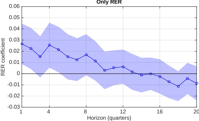
We also run long-horizon regressions of future excess returns on lagged 5-year changes in
RER, lagged fundamentals, and lagged returns
RXj,t+h =αh+βh∆(5y)qj,t+γhXj,t+δhRXj,t+τt+h+uj,t+h (6)
for forecast horizons of h= 1,2, ...,20 quarters. This regression also allows for lagged excess
returns as an additional control. The sequence of estimated βh coefficients can be thought
of as the impulse-response function of excess returns to long-run changes in the RER while
holding the path of macro fundamentals constant – a method known as local projections
(see Jorda, 2005). Results for a specification where we do not include controls (γ = 0) are
shown in the upper part of Figure 1, whereas the lower part of that figure shows results when
controls are included. In both cases, we plot the sequence of estimated βh coefficients and
95% confidence intervals based on clustered standard errors (clustered by time).
– Figure 1 about here –
Similar to the results in Table 3 discussed above, we find that return predictability by the
5-year RER change strengthens when controlling for macro fundamentals. The predictive
coefficient is higher at all horizons h, and predictability is much more persistent and extends
to about two years when controlling for fundamentals. By contrast, when fundamentals are
Next, we test the above relations in a portfolio setting. This allows for a direct
imple-mentation of trading strategies and to infer the economic value of the predictive relationship.
3.4 Currency value strategies
3.4.1 Constructing currency value portfolios
In our benchmark setup, we build currency portfolios with linear weights given by
wj,t+1 =ct(xj,t−xt), (7)
where xj,t denotes the signal for currency j in quarter t (such as the RER) and xt =
Nt−1ΣNt
j=1xj,t denotes the cross-sectional average of this signal (across countries, Nt). ct
is a scaling factor such that the absolute sum of all portfolio weights equals unity, i.e.,
ct = 1/
P
j|xj,t −xt|. Currencies with a value of the signal above the cross-sectional mean
receive positive portfolio weights, whereas currencies with a below-average value receive
neg-ative weights. The portfolio return rxp is then given by rxp t+1 =
PNt
j=1wj,t+1rxj,t+1. In the
implementation of this approach we re-balance the portfolios at the end of each quarter.
This setup where weights are linear in the signal is simple, but very useful for decomposing
the overall portfolio return into different components of the signal. For example, suppose we
can decompose a signal xj,t into two components such that xj,t = x1,j,t +x2,j,t; then the
returns to the two portfolios based on w1,j,t+1 =ct(x1,j,t−x1,t) and w2,j,t+1 =ct(x2,j,t−x2,t)
will add up to the overall portfolio return based on the composite signal xj,t defined above.
This allows us to perform simple decompositions of the predictive information in currency
value into different underlying components. However, due to the decomposition of the signal,
the absolute amount invested in each currency for each signal can differ from the absolute
In addition to the benchmark results with linear weights, we also report returns of rank
portfolios (see, e.g., Asness, Moskowitz, and Pedersen, 2012), where weights are given by
wj,t+1 =ct rank(xj,t)− Nt
X
j=1
rank(xj,t)/Nt
!
. (8)
The scaling factorctis analogous to the case of linear weights above (but uses ranks of signals
instead of actual signals) and ensures that we are one dollar long and dollar short as in Asness,
Moskowitz, and Pedersen (2012). This procedure is more conservative (in that outliers and
other extreme scores of signals receive a smaller weight) and does not have the effect discussed
above that the absolute amount invested changes across signals, but the downside is that it
does not permit exact decompositions.
Finally, we also perform standard cross-sectional portfolio sorts for comparison, sorting
currencies into four bins (P1, P2, P3, P4) based on quartiles of the cross-sectional distribution
of real exchange rates. Within each bin, currencies are equally weighted (as, e.g., in Lustig,
Roussanov, and Verdelhan, 2011; Menkhoff, Sarno, Schmeling, and Schrimpf, 2012a). We
report results for a high-minus-low portfolio (HM L) long in P4 (weak real exchange rates)
and short in P1 (strong real exchange rates).
3.4.2 Benchmark results
We start by building benchmark value portfolios sorted on the 5-year change in the RER,
∆(5y)q
j,t. The results are shown in Table 4.
– Table 4 about here –
We find that standard value portfolios deliver statistically significant positive excess
re-turns which also seem economically significant. Sharpe Ratios range between 0.44 and 0.51
magnitude as in Asness, Moskowitz, and Pedersen (2012).
3.4.3 Currency value strategies accounting for macroeconomic fundamentals
We then report results for modified value strategies in Table 5 where we purge ∆(5y)q of the
impact of macro fundamentals, based on the intuition in Eq. (4). We do so by running cross-sectional regressions of value signals (5-year RER changes) on our set of four fundamentals or expected fundamentals (xt) separately in each quarter t of our sample period
∆(5y)qj,t =αt+βtxj,t+εQj,t, (9)
where j indexes currencies as above. This gives us a fitted value signal (which we denote by
\
∆(5y)q in the following for ease of notation) and the residual value signal after stripping out
the impact of (expected) fundamentals on the RER, denoted εq. We are mainly interested
in the residual value signal, which serves as a measure of currency value when controlling for
the effect of (expected) fundamentals on the RER.
We examine four different variants of this basic setup. First, we simply regress 5-year
RER changes on macro fundamentals directly in each quarter. We save the fitted value of the
residual for each quarter and build linear and rank portfolios based on this decomposition of
the value signal. Panel A of Table 5 refers to this case. Second, we use exponentially weighted
moving averages of all fundamentals to proxy for expected fundamentals (Panel B).9We then
run cross-sectional regressions of the value signal on these proxies for expected fundamentals
9We approximate expectations as discounted long-run growth rates of some macro fundamental as
e
gt =
P∞
j=0φ jg
t−j
/P∞
j=0φ
j, and then use
e
and, again, sort currencies into portfolios based on either the fitted value or the residual.
The third case, in Panel C, uses a simple VAR(1) of all fundamentals to compute a proxy
for expected fundamentals. We estimate VARs separately for each country and recursively
based on an initialization window from 1970Q1 to 1975Q4. Expected fundamentals are then
obtained from iterating the VAR forward (and truncating after 20 quarters). These expected
fundamentals are then used in Eq. (9) to decompose the value signal. Finally, Panel D shows
results for a setup where we estimate a panel VAR for all countries jointly. Apart from this,
the procedure is the same as for the individual country VARs discussed above.
– Table 5 about here –
Table 5 shows annualized mean returns,t-statistics based on White (1980) standard errors,
return volatilities, and Sharpe Ratios for linear (left) and rank (right) portfolios, and for a
portfolio based on the 5-year change in the RER (∆(5y)q), the fitted signal (∆\(5y)q), and the
residual signal (εq). We always report returns for the benchmark value signal (∆(5y)q) for
comparison since including different combinations of macro variables changes the available
sample period.
For all four cases in Panels A–D, we find that adjusting the RER for macro fundamentals
increases the Sharpe Ratio substantially relative to the baseline case. This effect is not
driven by higher mean returns but rather by lowering return volatilities.10 This can also
be seen clearly from plots of cumulative returns to rank portfolios in Figure 2 where we
plot cumulative returns to the standard value strategy (based on 5-year RER changes) and
cumulative returns to modified value strategies (based on εQ).11 One way to interpret this
finding is that purging the value signal of the impact of (expected) fundamentals results in a
more precise measure of expected risk premiums, consistent with the intuition developed in
10Moreover, this result is true for both linear and rank portfolios. Hence it is not purely driven by investing less (in absolute terms) in the linear weight portfolios.
Section 2.2.
– Figure 2 about here –
This effect translates into other measures of risk which also tend to improve when
ad-justing for macroeconomic fundamentals. For example, we plot the drawdown dynamics of
standard value portfolios (∆(5y)q) and modified value portfolios (εq) based on rank weights.
We employ returns based on the panel VAR specification in Panel D of Table 5 in Figure 3.
We compute the drawdown Dt in quarter t based on rank portfolio returns as
Dt = t
X
s=1
rxps− max
u∈{1,...,t}
u
X
s=1
rxps (10)
where rxp is the portfolio excess return of the standard value portfolio (based on 5-year
RER changes) or of the modified value portfolio (based on εq).12 Figure 3 clearly shows that
adjusting for fundamentals reduces downside risk of the currency value strategy substantially.
– Figure 3 about here –
3.4.4 Exposure to other currency risk factors
Next, we explore how the value strategies relate to other well-established common factors
in currency markets. To do so, we run regressions of value returns adjusted for expected
fundamentals (based on the panel VAR in Panel D of Table 5) on returns to carry, momentum,
standard value (based on 5-year RER changes), and the global imbalance (IMB) factor of
Della Corte, Riddiough, and Sarno (2016). The latter is available from 1983Q4 onwards only,
so we run separate regressions with this factor. Results are shown in Panel A of Table 6.
– Table 6 about here –
We find that the modified value strategy (εq) that strips out the impact of expected macro
fundamentals delivers significant alphas across all specifications and even when including
standard value factors in the regression (specifications (iii) and (vi)). Information ratios are
quite high, ranging from 0.53 to 0.91 (annualized). Finally, Panel B of Table 6 shows weights
of the different strategies in the tangency portfolio. The modified value strategy gets a large
and significant weight in all specifications. It even exceeds that of the classical carry trade,
the currency strategy which has received most of the focus in the literature so far.13
4
Additional results and robustness
4.1 Macro fundamentals and real exchange rates in the cross section
To further understand the link between macro fundamentals and value signals, we run panel
regressions of 5-year RER changes on our set of macro fundamentals. We include time fixed
effects and inference is based on two-way clustered standard errors (clustered by currency
and quarter). Table 7 shows that higher productivity (HBS), higher export quality, higher
net foreign assets, and larger output gaps are associated with stronger real exchange rates
(i.e. a lower q in our notation).
– Table 7 about here –
Except for NFA, all fundamentals enter significantly into the various regression
specifica-tions.14 However, the R2 is at most 33% (for specification (ii)), so a substantial share of the
cross-sectional dispersion in value signals is left unexplained. Our results above suggest that
13Weights are calculated for an ex-post tangency portfolio to show that that ex-post the efficient frontier would include the modified value strategy with a large weight. This does not necessarily imply an expansion of the ex-ante frontier but, given the large weight attributed to value, this possibility seems most likely.
this unexplained part is largely driven by expected excess returns (currency risk premiums).
4.2 Decomposing value signals
To shed light on the mechanics of currency value strategies and to further understand the
drivers of return predictability, we further decompose the RER level into several
compo-nents. Specifically, we first split the information in the log RER level (qt) into that in the
lagged 5-year RER level (qt−5y) and the 5-year change in the RER ∆(5y)qt.15 With this basic
decomposition at hand, we then split the information content of 5-year RER changes into
the parts attributable to the (negative) 5-year spot rate change ∆(5y)st and (negative)
5-year inflation differential ∆(5y)πt∗, respectively. This decomposition tells us whether lagged
RER levels or changes drive return predictability and whether return predictability by the
5-year RER change stems from the spot rate component or inflation differentials. We build
linear portfolios which allow for an exact decomposition of returns, and rank portfolios for
robustness. Results are presented in Table 8.
– Table 8 about here –
Results based on the exact decomposition with linear portfolio weights in Panel A show
that around 60% of the excess return predictability from the RER level comes from 5-year
changes in the RER, i.e., the standard value signal in this paper and the literature (Asness,
Moskowitz, and Pedersen, 2012; Kroencke, Schindler, and Schrimpf, 2014; Barroso and
Santa-Clara, 2015). The remainder comes from the 5-year lagged level (which is not statistically
significant though). Hence, using 5-year RER changes seems to capture the predictive power
of RER for currency returns well. Furthermore, we find that lagged inflation differentials
and lagged 5-year spot exchange rate changes have opposite predictive power for currency
returns. Going long the currencies of countries with high inflation (relative to the U.S.)
forecasts positive excess returns relative to low inflation countries. This suggests that there
might be a risk premium for high inflation countries. For the spot rate component, we find
that going long countries with high 5-year appreciation rates forecasts low excess returns
relative to currencies which depreciated over the last 5 years. Strong currencies thus tend to
earn low risk premiums going forward.
4.3 Carry and value: Sequential sorts
A standard benchmark strategy in currency markets is the carry trade, which goes long
cur-rencies with high interest rates and short curcur-rencies which offer low interest rates (see, e.g.,
Lustig and Verdelhan, 2007; Brunnermeier, Nagel, and Pedersen, 2009; Burnside,
Eichen-baum, Kleshchelski, and Rebelo, 2011). To better understand the link between carry and
value, we form sequential portfolios where we first, in each quarter, split the set of available
currencies into two baskets (along the median) according to one signal. Then, we form rank
portfolios within these two baskets based on a second signal.
Table 9 reports results for this exercise. The left part of the table reports returns to value
portfolios built within buckets of currencies with high or low carry whereas the right part of
the table refers to carry portfolios built within baskets of currencies with high or low value.
– Table 9 about here –
The results suggest that, judging from the Sharpe Ratio, carry strategies tend to perform
slightly better among currencies with high value (i.e., low valuation). Value strategies, by
contrast, work better among low carry currencies. The differences in Sharpe Ratios are small
in economic terms, though. A reasonable conclusion is that value and carry capture largely
4.4 Home bias and real exchange rates
Another factor that should be related to real exchange rates (e.g., Warnock, 2003) is home bias
in trade. The intuition is that countries with stronger home bias have a stronger preference
for domestic goods. Stronger home bias then becomes a friction that prevents PPP from
holding and, in particular, leads to higher price levels in the country with stronger home
bias. Hence, one should observe a stronger RER for countries with stronger home bias in
goods markets.
We tackle this question by means of two different measures of home bias: (i) home bias
in trade and, for robustness, (ii) home bias in equity investments.16 To measure home bias in
trade, we simply rely on import shares (imports divided by nominal GDP) as in Heathcote
and Perri (2013). These data are available from the GFD as well. Home bias in equity
investments is measured via the IMF’s Coordinated Portfolio Investment Survey (CPIS).
The main idea of the asset market home-bias measure is to relate a country’s foreign asset
holdings to the weights of foreign assets that investors would need to hold if the International
Capital Asset Pricing Model was their point of reference. These data are available at annual
frequency from 2001 onwards. The construction of this asset market home-bias measure is
fairly standard (e.g., Fidora, Fratzscher, and Thimann, 2007).
Table A.I in the Internet Appendix reports results for panel regressions (with time fixed
effects) where we regress our value signal on one or both of the two home bias measures, and
with and without including our other fundamentals as controls. As can be seen from
speci-fications (i) and (ii), a larger degree of home bias in trade is (counterintuitively) associated
with a higher value signal (i.e., a weaker RER). Yet, this link is not statistically significant.
Similarly, for the financial home bias measure we also find insignificant slope coefficients
(specifications (iii) and (iv)). Finally, specification (v) shows that both measures are
icant when included jointly in the regression and when controlling for the other fundamentals.
Conventional measures of home bias thus do not seem to drive the cross-sectional variation
of currency value in our sample.
4.5 Value portfolios based on absolute PPP
Our benchmark value signal is based on 5-year changes in RER levels computed from spot
exchange rates and CPI inflation, normalized to unity in 1970Q1. For robustness, we also
compute portfolio returns based on a measure of the RER that is immune to the base year
choice and computed from actual disaggregated product prices. These data are taken from
the OECD but are only updated every three years. Another downside is that the OECD
data are available at annual frequency only and cover a smaller set of currencies. Hence, we
only use these data for robustness. Table A.II in the Internet Appendix shows results for
portfolios based on 5-year changes in RERs computed from absolute PPP measures and we
find that the results are similar to those in Table 4.
4.6 Cross-validation: Influential currencies
To rule out the possibility that the main results are driven by one particular currency, we
provide results from a cross-validation exercise in Table A.III in the Internet Appendix. More
specifically, we drop one currency at a time, control for macro fundamentals, and compute
returns to the modified value strategy (εq) as in Table 5. The rows in Table A.III indicate
which currency was excluded from the sample. Overall, we find that the results are robust
and are not driven by one particular outlier currency.
4.7 Average portfolio weights
We document average rank portfolio weights in Table A.IV for all currencies in our sample.
For example, we find that Sweden, South Korea, and Canada consistently get high positive
weights across the four methods, whereas countries such as New Zealand, Hungary, Japan,
and Switzerland get low weights. The table also shows that the volatility of portfolio weights
is around 11% so it is not the case that our value measures always select the same currencies
for going long and short, respectively.17
4.8 Implementation lags
We repeat the analysis underlying Table 5 and build currency portfolios based on value
signals purged from expected fundamentals. However, we allow for an additional two quarters
between observing the signals and forming the portfolio, i.e. we add an implementation lag of
two quarters to account for the fact that macroeconomic variables are reported with a lag.18
While lagging the value signal clearly reduces mean excess returns and Sharpe Ratios for all
portfolios, we still find the same general pattern in portfolio returns as in our benchmark
analyses above: Portfolios based on raw value signals (RER) have clearly lower average
returns and Sharpe Ratios than portfolios based on controlling for expected fundamentals
(εq). This result is also related to our finding in Figure 1 above, which shows that controlling
for fundamentals leads to more persistent predictability than using the raw value signal
(5-year RER changes).
17The volatility of rank portfolio weights can be interpreted as a measure of portfolio turnover. However, a more intuitive way to gauge this is to use portfolio weight changes to compute actual turnover numbers. For our modified value strategy based on panel VARs, we find a quarterly turnover rate of about 21%. For comparison, turnover for a standard carry strategy is close to 10%, for momentum it is 60%, and for a standard value strategy it is about 18%.
5
Conclusion
The valuation of currencies is of key importance to international investors, but empirical
evidence on the properties and determinants of “currency value” is still scattered in the
literature and largely incomplete. This is unfortunate as currency value measures based on
the real exchange rate are commonly used for practical purposes, e.g. when gauging currency
misalignments or for the design of currency investment and hedging strategies.
We contribute to the literature by investigating the predictive content of real exchange
rates as well as real exchange rates adjusted for macroeconomic fundamentals for future
currency excess returns. Our ultimate goal is to provide a better understanding of the link
between currency valuation and risk premiums in the cross-section of currencies. We find that
real exchange rates predict the cross-section of currency excess returns. A more powerful value
signal can be obtained, however, when adjusting real exchange rates for key fundamentals
(productivity, export quality, net foreign assets, and output gaps) – well-known from the
macro exchange rate literature but hitherto unexplored in asset pricing research. Finally,
portfolios based on standard and modified value signals should also be useful for research
on currency risk factors in the cross-section as they offer a set of returns that are largely
independent of carry and momentum.
Overall, these results are encouraging given the well-known empirical difficulties of models
of exchange rate equilibrium, and should spur further research in several directions. Most
importantly, while this paper has a strong empirical asset pricing focus, our results have
implications for international macro models of exchange rate determination and for theoretical
work. An immediate avenue for further research is the development of a clear theoretical
framework that can fully specify the economic mechanisms that imply how a weak RER is
contemporaneously associated with a high currency risk premium. This could conceivably be
achieved, for example, by incorporating deviations from PPP in a model of rare disaster with
incomplete markets model with financial frictions of Gabaix and Maggiori (2015) to allow for
additional distortions due to non-homogeneity in traded goods and productivity differentials.
References
Asness, C. S., T. J. Moskowitz, and L. H. Pedersen (2012): “Value and Momentum
Everywhere,”Journal of Finance, 68, 929–985.
Balduzzi, P., and I. E. Chiang (2014): “Real Exchange Rates and Currency Risk
Pre-mia,” Working Paper, Boston College.
Barroso, P., and P. Santa-Clara(2015): “Beyond the Carry Trade: Optimal Currency
Portfolios,”Journal of Financial and Quantitative Analysis, 50, 1037–1056.
Brunnermeier, M., S. Nagel, and L. Pedersen (2009): “Carry Trades and Currency
Crashes,”NBER Macroeconomics Annual 2008, 23, 313–347.
Burnside, C., M. Eichenbaum, I. Kleshchelski, and S. Rebelo (2011): “Do Peso
Problems Explain the Returns to the Carry Trade?,” Review of Financial Studies, 24, 853–891.
Chong, Y., O. Jorda, and A. Taylor (2012): “The Harrod-Balassa-Samuelson
Hy-pothesis: Real Exchange Rates and their Long-Run Equilibrium,”International Economic Review, 53, 609–634.
Cieslak, A., and P. Povala (2016): “Expected Returns in Treasury Bonds,”Review of
Financial Studies, 29, 2859–2901.
Clarida, R. H., J. Gali, and M. Gertler(2000): “Monetary Policy Rules and
Macroe-conomic Stability: Evidence and Some Theory,” Quarterly Journal of Economics, 115, 147–180.
Cooper, I., and R. Priestley (2009): “Time-Varying Risk Premiums and the Output
Gap,”Review of Financial Studies, 22(7), 2801–2833.
Della Corte, P., S. Riddiough, and L. Sarno (2016): “Currency Premia and Global
Imbalances,”Review of Financial Studies, forthcoming, doi:10.1093/rfs/hhw038.
Engel, C. (2016): “The Real Exchange Rate, Real Interest Rates, and the Risk Premium,”
American Economic Review, 106, 436–474.
Engel, C., and K. D. West (2005): “Exchange Rates and Fundamentals,”Journal of
Political Economy, 113, 485–517.
(2006): “Taylor Rules and the Deutschmark-Dollar Real Exchange Rate,”Journal of Money, Credit and Banking, 38, 1175–1994.
Evans, G., and S. Honkapohja (2009): “Learning and Macroeconomics,”Annual Review
of Economics, 1, 421–449.
Farhi, E., and X. Gabaix(2016): “Rare Disasters and Exchange Rates,”Quarterly Journal
Fidora, M., M. Fratzscher, and C. Thimann (2007): “Home Bias in Global Bond
and Equity Markets: The Role of Real Exchange Rate Volatility,”Journal of International Money and Finance, 26, 631–655.
Froot, K. A., and T. Ramadorai (2005): “Currency Returns, Intrinsic Value, and
Institutional-Investor Flows,”Journal of Finance, 60, 1535–1566.
Gabaix, X., and M. Maggiori (2015): “International Liquidity and Exchange Rate
Dy-namics,”Quarterly Journal of Economics, 130, 1369–1420.
Gerakos, J., and J. T. Linnainmaa (2016): “Average Returns, Book-to-Market, and
Changes in Firm Size,” Working Paper, Chicago Booth.
Gourinchas, P.-O., and H. Rey (2007): “International Financial Adjustments,”Journal
of Political Economy, 115, 665–703.
Hassan, T., and R. Mano(2015): “Forward and Spot Exchange Rates in a Multi-Currency
World,” Working Paper, Chicago Booth.
Heathcote, J., and F. Perri (2013): “The International Diversification Puzzle Is Not as
Bad as You Think,”Journal of Political Economy, 121, 1108–1159.
Henn, C., C. Papageorgiou, and N. Spatafora (2013): “Export Quality in Developing
Countries,” IMF Working Paper.
Heyerdahl-Larsen, C.(2014): “Asset Prices and Real Exchange Rates with Deep Habits,”
Review of Financial Studies, 27, 3280–3317.
Hummels, D., and P. J. Klenow(2005): “The Variety and Quality of a Nation’s Exports,”
American Economic Review, 95, 704–723.
Jorda, O. (2005): “Estimation and Inference of Impulse Responses by Local Projections,”
American Economic Review, 95, 161–182.
Jorda, O., and A. Taylor(2012): “The Carry Trade and Fundamentals: Nothing to Fear
but FEER Itself,”Journal of International Economics, 88, 74–90.
Koijen, R. S., T. J. Moskowitz, L. H. Pedersen, and E. B. Vrugt(2015): “Carry,”
Working Paper, London Business School.
Kozicki, S., and P. Tinsley (2005): “Permanent and Transitory Policy Shocks in an
Empirical Macro Model with Asymmetric Information,”Journal of Economic Dynamics and Control, 29, 1985–2015.
Kroencke, T. A., F. Schindler, and A. Schrimpf (2014): “International
Diversi-fication Benefits with Foreign Exchange Investment Styles,” Review of Finance, 18(5), 1847–1883.
Lane, P. R., and G. M. Milesi-Ferretti (2004): “The Transfer Problem Revisited:
(2007): “The External Wealth of Nations Mark II: Revised and Extended Estimates of Foreign Assets and Liabilities, 1970–2004,” Journal of International Economics, 73, 223–250.
Lettau, M., M. Maggiori, and M. Weber (2014): “Conditional Risk Premia in
Cur-rency Markets and Other Asset Classes,”Journal of Financial Economics, 114, 197–225.
Lustig, H., N. Roussanov, and A. Verdelhan (2011): “Common Risk Factors in
Currency Markets,”Review of Financial Studies, 24, 3731–3777.
Lustig, H., and A. Verdelhan (2007): “The Cross Section of Foreign Currency Risk
Premia and Consumption Growth Risk,”American Economic Review, 97, 89–117.
Melvin, M., and D. Shand (2013): “Forecasting Exchange Rates: an Investor
Perspec-tive,” in Handbook of Economic Forecasting, ed. by G. Elliott,and A. Timmermann. Else-vier, vol. 2, p. 721:750.
Menkhoff, L., L. Sarno, M. Schmeling, and A. Schrimpf (2012a): “Carry Trades
and Global Foreign Exchange Volatility,”Journal of Finance, 67, 681–718.
(2012b): “Currency Momentum Strategies,”Journal of Financial Economics, 106, 660–684.
(2016): “Information Flows in Foreign Exchange Markets: Dissecting Customer Currency Trades,”Journal of Finance, 71, 601–633.
Molodtsova, T., A. Nikolsko-Rzhevskyy, and D. H. Papell (2008): “Taylor Rules
with Real-time Data: A Tale of Two Countries and One Exchange Rate,” Journal of Monetary Economics, 55, S63–S79.
Molodtsova, T., and D. Papell (2009): “Out-of-sample Exchange Rate Predictability
with Taylor Rule Fundamentals,”Journal of International Economics, 77, 167–180.
Piazzesi, M., and M. Schneider(2011): “Trend and Cycle in Bond Risk Premia,”
Work-ing Paper, Stanford GSB.
Pojarliev, M., and R. M. Levich (2010): “Trades of the Living Dead: Style Differences,
Style Persistence and Performance of Currency Fund Managers,”Journal of International Money and Finance, 29, 1752–1775.
Rogoff, K.(1996): “The Purchasing Power Parity Puzzle,”Journal of Economic Literature,
34, 647–668.
Rose, D. (2010): “The Influence of Foreign Assets and Liabilities on Real Interest Rates,”
Institute of Policy Studies Working Paper No. 10/09.
Sarno, L., and M. P. Taylor (2002): “Purchasing Power Parity and the Real Exchange
Rate,”IMF Staff Papers, 49, 65–105.
Stockman, A., and H. Dellas (1989): “International Portfolio Nondiversification and
Taylor, A., and M. Taylor (2004): “The Purchasing Power Debate,”Journal of
Eco-nomic Perspectives, 18, 135–158.
Taylor, J. B. (1993): “Discretion versus Policy Rules in Practice,” Carnegie-Rochester
Conference Series on Public Policy, 39, 195–214.
Vandenbussche, H. (2014): “Quality in Exports,” Economic Papers 528, European
Com-mission, Directorate General for Economic and Financial Affairs.
Warnock, F.(2003): “Exchange Rate Dynamics and the Welfare Effects of Monetary Policy
in a Two-Country Model with Home-Product Bias,”Journal of International Money and Finance, 22, 343–363.
White, H. (1980): “A Heteroskedasticity-Consistent Covariance Matrix Estimator and a
Table 2. Predictive power of macroeconomic fundamentals for real interest rate differentials
This table reports p-values for tests of a link between macro fundamentals and subsequent real interest rate differentials (RIDs). We adopt a Granger causality type setting and regress RIDs on lagged RIDs, real per-capita GDP (HBS), export quality (Qual), net foreign assets scaled by GDP (NFA), and output gaps (OG). h denotes the forecast horizon (years). The results are based on panel regressions which include time fixed effects (year fixed effects). t -statistics are based on two-way clustered standard errors (clustered by currency and quarter). The sample period is 1976 – 2013 and the frequency is annual.
h RID HBS Qual NFA OG
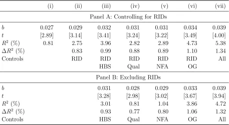
Table 3. Regressions of excess returns on 5-year RER changes and controls
This table reports results for panel regressions of excess returns on lagged 5-year RER changes and further control variables. These control variables include: real interest rate differentials (RID), real per-capita GDP (HBS), export quality (Qual), net foreign assets scaled by GDP (NFA), and output gaps (OG). We report the slope estimate (b) for 5-year RER changes, the associated t-statistic (in brackets), the (adjusted) R2 (in %), and the incremental R2
(denoted ∆R2) when adding 5-year RER changes to the regression. The upper panel shows results for specifications where the real interest rate is included in all specifications except (i). The lower panel excludes RIDs everywhere. The final rows of each panel indicate which control variables are included in the regression. All panel regressions include time fixed effects (quarterly basis). t-statistics are based on clustered standard errors (clustered by quarter). The sample period is 1976Q1 – 2014Q1 and the frequency is quarterly.
(i) (ii) (iii) (iv) (v) (vi) (vii)
Panel A: Controlling for RIDs
b 0.027 0.029 0.032 0.031 0.031 0.034 0.039
t [2.89] [3.14] [3.41] [3.24] [3.22] [3.49] [4.00]
R2 (%) 0.81 2.75 3.96 2.82 2.89 4.73 5.38
∆R2 (%) 0.83 0.99 0.88 0.89 1.10 1.34
Controls RID RID RID RID RID All
HBS Qual NFA OG
Panel B: Excluding RIDs
b 0.031 0.028 0.029 0.033 0.039
t [3.28] [2.98] [3.02] [3.67] [3.94]
R2 (%) 3.01 0.81 1.04 3.86 4.72
∆R2 (%) 0.93 0.77 0.80 1.06 1.32
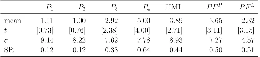
Table 4. Returns to currency value strategies
This table reports descriptive statistics for currency portfolios based on 5-year real exchange rate changes. We report results for cross-sectional portfolio sorts where we sort currencies into 4 bins based on the cross section of signals (portfolios P1, ..., P4 and a high minus low
portfolio, HML, long P4 and short P1), as well as a rank portfolio (P FR), and a simple
portfolio based on linear portfolio weights (P FL; weights are linear in the cross-sectional
deviation of signals from the cross-sectional mean). Real exchange rates are defined such that a higher real exchange rate indicates a weaker foreign currency. Hence, the portfolios go long currencies currencies that are relatively cheap and goes short currencies with valuations that have become relatively rich. Excess returns are defined such that positive numbers mean a positive return on holding the foreign currency. Mean returns, return volatilities (σ), and Sharpe Ratios (SR) are annualized. t-statistics in brackets are based on White (1980) standard errors. The sample period is 1976Q1 – 2014Q1 and the frequency is quarterly.
P1 P2 P3 P4 HML P FR P FL
mean 1.11 1.00 2.92 5.00 3.89 3.65 2.32
t [0.73] [0.76] [2.38] [4.00] [2.71] [3.11] [3.15]
σ 9.44 8.22 7.62 7.78 8.93 7.27 4.57
Table 5. Currency value strategies accounting for fundamentals
This table reports excess returns for portfolios formed on 5-year RER changes (∆(5y)q) and
a decomposition into the part of ∆(5y)q related to macro fundamentals (∆\(5y)q) and a part
unrelated to these fundamentals (εq). We regress ∆(5y)q on real per-capita GDP, export
quality, net foreign assets scaled by GDP, and output gaps in the cross-section each quarter to obtain the fitted RER (∆\(5y)q) and the residual (εq). We then build linear-weight and rank
portfolios based on these two components. We use four different measures of fundamentals in these cross-sectional regressions: Panel (a) simply uses the raw fundamentals whereas the remaining panels use proxies for expected fundamentals. Panel (b) uses an exponentially-weighted moving average (EWMA), Panel (c) employs expected fundamentals from VARs (estimated recursively and separately for each country), and Panel (d) uses a (recursive) panel VAR to compute expected fundamentals. We report annualized mean excess returns,
t-statistics based on White (1980) standard errors in squared brackets, the annualized excess return volatility (σ), and annualized Sharpe Ratios (SR). The sample period is 1976Q1 – 2013Q4 (at most) and the frequency is quarterly.
Linear portfolios Rank portfolios
∆(5y)q ∆\(5y)q εq ∆(5y)q ∆\(5y)q εq
Panel A. Raw fundamentals
mean 2.67 0.54 2.13 4.16 2.05 4.12
t [3.35] [0.93] [4.91] [3.27] [1.47] [4.89]
σ 4.93 3.61 2.68 7.85 8.61 5.22
SR 0.54 0.15 0.79 0.53 0.24 0.79
Panel B. Expected fundamentals (EWMA)
mean 3.00 0.26 2.74 4.67 1.23 4.76
t [3.41] [0.42] [5.21] [3.35] [0.85] [4.71]
σ 5.10 3.56 3.04 8.06 8.40 5.85
SR 0.59 0.07 0.90 0.58 0.15 0.81
Panel C. Expected fundamentals (VAR)
mean 3.04 0.82 2.22 4.76 2.88 4.86
t [3.51] [1.24] [4.97] [3.46] [1.87] [5.32]
σ 5.08 3.87 2.62 8.05 9.02 5.35
SR 0.60 0.21 0.85 0.59 0.32 0.91
Panel D. Expected fundamentals (Panel VAR)
mean 3.04 0.61 2.43 4.76 2.37 4.67
t [3.51] [0.95] [5.32] [3.46] [1.54] [5.26]
σ 5.08 3.77 2.68 8.05 9.00 5.19
Table 6. Currency value: Exposure regressions
This table reports exposure regression results in Panel A and weights in global tangency port-folios in Panel B. The dependent variable in Panel A is the excess return of a value portfolio based on 5-year RER changes controlling for macro fundamentals (see Panel D in Table 5). As factors in the regressions, we include excess returns to carry trades, momentum, standard value (based on 5-year RER changes, ∆(5y)q), and the global imbalances factor (IM B) of
Della Corte, Riddiough, and Sarno (2016) in various different specifications. R2 denotes the
(adjusted) regressionR2 whereasIRdenotes the information ratio (alpha divided by residual
standard deviation). Alphas and information ratios are annualized and in percent. The sam-ple period is 1980Q3 – 2013Q1 for all specifications not involving IM B and 1983Q4-2013Q4 for specifications involving IM B due to data availability. Numbers in squared brackets are
t-statistics based on White (1980) standard errors.
(i) (ii) (iii) (iv) (v) (vi)]
Panel A. Exposure regressions
α 4.67 4.62 2.31 4.09 3.60 2.06
[5.26] [4.97] [2.92] [4.43] [3.75] [2.35]
Carry 0.06 0.07 0.13 0.12
[0.99] [1.34] [1.97] [2.09]
Mom -0.12 0.03 -0.14 0.03
[-1.84] [0.65] [-2.34] [0.52]
∆(5y)q 0.45 0.44
[8.70] [7.48]
IM B 0.07 0.07 0.01
[0.84] [0.90] [0.17]
R2 2.97 39.59 -0.05 7.07 40.60
IR 0.90 0.91 0.58 0.80 0.73 0.53
Panel B.Tangency portfolio weights
Carry 0.32 0.22 0.22 0.22 0.22
[3.78] [2.77] [2.97] [2.96] [3.17]
Mom 0.30 0.19 0.21 0.15 0.16
[3.07] [2.41] [2.37] [2.14] [1.91]
∆(5y)q 0.38 0.13 0.04
[3.19] [0.88] [0.34]
IM B 0.35 0.24 0.23
[2.93] [3.42] [3.06]
εq 0.59 0.45 0.65 0.39 0.35
Table 7. Macroeconomic fundamentals as drivers of real exchange rates
This table reports results for panel regressions of 5-year RER changes on macro fundamentals. These fundamentals are: real per-capita GDP (HBS), export quality (Qual), net foreign assets scaled by GDP (NFA), and output gaps (OG). All panel regressions include time fixed effects (quarterly basis). t-statistics are based on two-way clustered standard errors (clustered by currency and quarter). The sample period is 1976Q1 – 2014Q1 and the frequency is quarterly. We report the simple R2 for specifications (i) – (iv) and the adjusted R2 for specification (v).
(i) (ii) (iii) (iv) (v)
HBS -0.11 -0.22
[-2.18] [-8.90]
Qual -0.32 -0.42
[-5.00] [-4.80]
NFA -0.02 0.02
[-0.72] [0.62]
OG -0.08 -1.04
[-1.79] [-7.65]
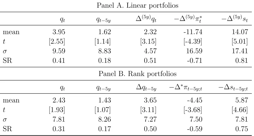
Table 8. Decomposing currency value signals
This table reports results for portfolios based on the RER level (qt), the lagged RER level 5 years ago (qt−5y), the 5-year change in the RER (∆(5y)qt), the negative of 5-year
infla-tion differentials (−∆(5y)π∗t), and the negative of 5-year nominal spot exchange rate changes (−∆(5y)st). Panel A shows results for linear portfolios where we can compute an exact de-composition of returns whereas Panel B shows results for rank portfolios. Portfolio weights are updated quarterly andt-statistics in brackets are based on White (1980) standard errors.
Panel A. Linear portfolios
qt qt−5y ∆(5y)qt −∆(5y)πt∗ −∆(5y)st
mean 3.95 1.62 2.32 -11.74 14.07
t [2.55] [1.14] [3.15] [-4.39] [5.01]
σ 9.59 8.83 4.57 16.59 17.41
SR 0.41 0.18 0.51 -0.71 0.81
Panel B. Rank portfolios
qt qt−5y ∆qt−5y −∆∗πt−5y;t −∆st−5y;t
mean 2.43 1.43 3.65 -4.45 5.87
t [1.93] [1.07] [3.11] [-3.68] [4.66]
σ 7.81 8.26 7.27 7.50 7.81
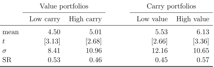
Table 9. Value vs. carry: Sequential portfolio sorts
This table reports results for sequential portfolios where we split the sample of currencies into two buckets depending on the median value of one characteristic in quarter t and then form rank portfolios separately within these two buckets according to a second characteristic and compute returns to these portfolios in quarter t+ 1. The results on the left (right) side of the table are based on first splitting the sample according to value (carry) and forming separate portfolios based on carry (value). Portfolios are updated quarterly. t-statistics in brackets are based on White (1980) standard errors. The sample period is 1976Q1 – 2013Q4 and the frequency is quarterly.
Value portfolios Carry portfolios
Low carry High carry Low value High value
mean 4.50 5.01 5.53 6.13
t [3.13] [2.68] [2.66] [3.36]
σ 8.41 10.96 12.16 10.65
Figure 1. Impulse-response functions: Excess returns
Horizon (quarters)
1 4 8 12 16 20
RER coefficient
-0.03 -0.02 -0.01 0 0.01 0.02 0.03 0.04 0.05
0.06 Only RER
Horizon (quarters)
1 4 8 12 16 20
RER coefficient
-0.03 -0.02 -0.01 0 0.01 0.02 0.03 0.04 0.05
0.06 Controlling for fundamentals
Figure 2. Cumulative excess returns to currency value strategies
1976 1981 1986 1991 1996 2001 2006 2011 Cumulative excess returns (in %) 0
0.5 1 1.5
Raw fundamentals
1981 1986 1991 1996 2001 2006 2011 Cumulative excess returns (in %) 0
0.5 1 1.5
Expected fundamentals (EWMA)
1980 1985 1990 1995 2000 2005 2010 Cumulative excess returns (in %) 0
0.5 1 1.5
Expected fundamentals (VAR)
1980 1985 1990 1995 2000 2005 2010 Cumulative excess returns (in %) 0
0.5 1 1.5
Expected fundamentals (Panel VAR)
This figure plots cumulative portfolio excess returns for value strategies. The blue solid lines refer to standard value strategies (based on 5-year RER changes) whereas the red dashed lines refer to modified value strategies (εQ) which control for (expected) macro fundamentals.