Emulation of utility functions over a set of permutations:
sequencing reliability growth tasks
Kevin J Wilson, Daniel A Henderson
School of Mathematics and Statistics, Newcastle University, UK and
John Quigley
Department of Management Science, University of Strathclyde, UK
August 29, 2017
Abstract
We consider Bayesian design of experiments problems in which we maximise the prior expectation of a utility function over a set of permutations, for example when sequencing a number of tasks to perform. When the number of tasks is large and the expected utility is expensive to compute, it may be unreasonable or infeasible to evaluate the expected utility of all permutations. We propose an approach to emulate the expected utility using a surrogate function based on a parametric probabilistic model for permutations. The surrogate function is fitted by maximising the correlation with the expected utility over a set of training points. We propose a suitable transformation of the expected utility to improve the fit. We provide results linking the correlation between the two functions and the number of expected utility evaluations to undertake. The approach is applied to the sequencing of reliability growth tasks in the development of hardware systems, in which there is a large number of potential tasks to perform and engineers are interested in meeting a reliability target subject to minimising costs and time. An illustrative example shows how the approach can be used and a simulation study demonstrates the performance of the approach more generally.
Keywords: Multi-attribute utility, Bayesian design of experiments, design for reliability, Benter model
1
Introduction
The maximisation of the prior expectation of a utility function to find the optimal design of an
ex-periment in a Bayesian analysis is challenging as a result of the necessity of evaluating the expected
utility for all designs. We can make progress by using an approximation based on a surrogate
func-tion which is faster to evaluate, known as an emulator [Kennedy and O’Hagan, 2001, Henderson
et al., 2009, Young and Ratto, 2011, Zhou et al., 2011]. When the possible experimental designs are
a set of permutations this adds complexity as commonly used emulators, such as Gaussian process
emulators, are based on the assumption of a smooth relationship between the inputs to, and outputs
from, the function being emulated, which is unlikely to be true in this case.
An example is the reliability growth of hardware products under development. During
develop-ment, initial designs are subject to detailed analysis, identifying improvements until performance
requirements are met. Reliability tasks which analyse the design and facilitate the enhancement
include fault tree analysis, failure modes and effects analysis and highly accelerated life testing.
These tasks can be resource intensive and costly to implement and each has the goal of design
im-provement by understanding weaknesses. Multiple tasks may uncover the same fault in the current
design of the product and some faults may not be uncovered by any of the tasks. Therefore, the
engineers are faced with the decision problem of which tasks to perform and in what order to grow
their reliability to the required level. Their possible experimental designs are the permutations of
the possible reliability tasks to carry out.
1.1 Emulation of permutations
The use of surrogate models for emulating expensive functions dates back at least as far as Sacks
et al. [1989] who propose a Gaussian process prior for the output of a complex computer model. An
early example of emulating an expensive utility function in the context of Bayesian optimal design is
described in M¨uller and Parmigiani [1995]. The use of surrogate models for emulating an expensive
function over a set of permutations has received relatively little attention. An early example is
described in Voutchkov et al. [2005] in which a surrogate model is proposed for ordering a sequence
of welding tasks in the aircraft industry. Most surrogate models for functions with continuous input
spaces, such as Gaussian processes or radial basis functions, are based on the premise that points
close in input space will lead to similar values of the expensive function. In terms of a generic
to replace the Euclidean distance between inputs in surrogate models with a more natural distance
measure on the space of permutations. This is the approach proposed by Moraglio and Kattan
[2011], Moraglio et al. [2011] and Kim et al. [2014]. These authors focused on a radial basis
function-based surrogate model for general combinatorial input spaces, including permutations.
They used the Hamming distance and Kendall tau distance as two distance measures on sets of
permutations; see Marden [1995] for details.
This approach of replacing the Euclidean distance with a permutation-based distance was
gener-alised by Zaefferer et al. [2014b] to a Gaussian process-based surrogate model. The use of a
Gaus-sian process-based surrogate allowed the authors to use the efficient global optimisation approach
of Jones et al. [1998] and a standard Kriging estimator. The authors reported improved performance
over a radial basis function-based surrogate on a set of combinatorial optimisation problems. This
work was extended by Zaefferer et al. [2014a] who investigated 14 different distance functions over
sets of permutations for Gaussian process-based surrogates. An approach based on choosing the
distance function by maximum likelihood yielded the best results, with the Hamming distance the
best single distance measure. Zaefferer [2015] describes an R package ‘CEGO’ for
implement-ing the Gaussian process-based surrogate modellimplement-ing and optimisation approach that is proposed in
Zaefferer et al. [2014b] and Zaefferer et al. [2014a].
1.2 Design for reliability
Design for reliability principles are not sufficient for designing complex systems [Wayne and
Modarres, 2015, U.S. Department of Defense, 2011, 2008] and as such reliability growth
contin-ues to provide a key role in product development. However, achieving growth through Test Analyse
And Fix (TAAF) is expensive which leads organisations to develop integrated programs of activities
to reduce reliance on testing [Krasich et al., 2004]. There are several activities employed to enhance
reliability during design and development, e.g. Highly Accelerated Life Testing (HALT), Fault Tree
Analysis, Failure Modes and Effects Analysis (FMEA) (see Blischke and Murthy [2011]), each of
which requires resources and must be managed, see for example IEC 61014. While these activities
have different perspectives upon a design, each has the common goal of seeking to improve the
design. To date, little attention has been paid in the literature on optimally sequencing activities to
achieve target reliability while minimising costs.
Past research has focused primarily on either determining optimal designs, for example with
rate from TAAF tests, for which there is international standard IEC 61164, comprising both
fre-quentist and Bayesian methods [Crow, 1974, Walls and Quigley, 1999, Quigley and Walls, 2003].
Research at the program level is scarce, either focusing on monitoring progress graphically
[Kra-sich, 2015, Walls et al., 2005] or project management issues such a metrics, infrastructure and
documentation [Eigbe et al., 2015]. While minimising program costs has been explored by Hsieh
and Hsieh [2003], Hsieh [2003] a key shortcoming has been the representation of growth and
pro-gram costs through continuous functions as decisions are discrete and choices are finite [Guikema
and Pate-Cornell, 2002]. An exception to this is Johnston et al. [2006] who explored minimising
program cost with discrete choices through integer programming methods and Wilson and Quigley
[2016] who provided a solution incorporating multi-attribute utility functions to allow trade-offs
between attributes; however neither paper addressed the issue of sequencing the activities.
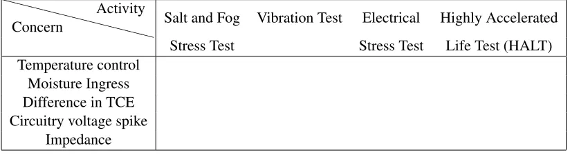
Table 1 provides a simplified illustrative example which is similar to practice but substantially
reduced in size and presented without industrially sensitive design details. Table 1 presents five
engineering concerns with the design of an aerospace system and four development activities; these
were identified through an elicitation process.
XX XX
XX XX
XXX
Concern
Activity
Salt and Fog Vibration Test Electrical Highly Accelerated
Stress Test Stress Test Life Test (HALT)
Temperature control Moisture Ingress Difference in TCE Circuitry voltage spike
[image:4.612.100.512.371.485.2]Impedance
Table 1: Illustrative efficacy matrix with 5 concerns and 5 activities
The ability of the design to maintain its temperature within acceptable limits was a concern
for the engineers, and while the current design may achieve desired control, the engineers were
uncertain. Moisture ingress was a concern as new material was being used in the design compared
with heritage designs and, while preliminary tests indicated that the new material would not be
deficient in this regard, the engineers were uncertain. The significance of the difference of the
Temperature Coefficient of Expansion (TCE) between different materials was a concern for aspects
of the system as this may prove to be a deficiency in the design. The possibility of aspects of the
circuitry generating unacceptable voltage spikes was identified. The final concern listed related
to uncertainty between the soldering, the environment and the circuits, where residue remaining
Associated with each concern is a probability that the concern is a fault, i.e. if the system were used
in operation it would fail due to an imperfection or deficiency described by the concern.
There are a variety of reliability tests that can be conducted to assess an item’s design at the
com-ponent, sub-assembly or system level; these include life and environment tests, for example Highly
Accelerated Life Testing (HALT), as well as environmental testing against specific stresses such
as vibration, heat, electricity, salt, fog or moisture. For a more detailed discussion see O’Connor
and Kleyner [2012] or Silverman [1998]. Table 1 presents four such activities and within each cell
of the table we would input a probability measuring how likely the associated activity would be to
identify the associated concern as a fault, assuming that the concern was a fault, i.e. the probability
it does not slip through test undetected.
Once populated with probabilities, efficacy matrices can help identify if there are concerns with
no associated activities and can form the basis of a reliability growth programme. Typically, the
matrices have a many to many relationship, where a fault can be exposed by several activities and
an activity can expose several faults. As such, there are choices to be made with respect to which
activities should be scheduled, with the aim of either identifying the faults in the design or providing
evidence that the concern is not a fault. While we have presented a simple example, a large system
design may have hundreds of concerns with as many activities.
1.3 This paper
In this paper we initially consider the problem of emulating the prior expectation of a utility function
over a set of permutations. We propose an approach to perform the emulation using the Benter
model [Benter, 1994] as the basis for the surrogate function. The Benter model is an extension of the
Plackett-Luce model [Plackett, 1975, Luce, 1959], a popular probabilistic model for permutations;
see [Marden, 1995] for further background on probabilistic models for permutations. We outline
how to fit the Benter model based on a training sample of model runs for the expected utility and
propose suitable transformations of both the expected utility and surrogate function to improve the
fit. We give results which provide us with a method of deciding on the number of evaluations of the
expected utility to make based on the optimal values of the surrogate function.
We consider the problem of sequencing reliability growth tasks specifically. We adapt a
com-monly used model for reliability growth [Johnston et al., 2006, Quigley and Walls, 2006] under
development to incorporate explicitly uncertainty on the reliability function and utilise this to
will stop testing when we reach a reliability target. We propose a two-attribute utility function to
solve the design of experiments problem.
In Section 2 we outline our general approach to emulation of the expected utilities on sets of
per-mutations and give theoretical results. In Section 3 we consider the model for reliability growth and
develop the solution to the decision problem. In Section 4 we give an illustrative example informed
by work with industrial partners in the aerospace industry. Section 5 considers two simulation
stud-ies to examine the strengths and weaknesses of the emulator more generally and provide guidance
on the choice of training and evaluation set sizes for the emulator. In Section 6 we summarise and
give some areas for further work.
2
Emulation of utility functions on permutations
2.1 The emulator
Suppose that there areJtasks which are to be performed in a sequence. Then there areJ!possible sequences, or permutations, of theJ tasks. LetSJdenote the set of all permutations of theJ tasks.
Each sequence of tasksx= (x1, x2, . . . , xJ)∈ SJ, wherexkdenotes thek’th task, gives rise to an
expected utilityu=U(x)∈[0,1], where 0 represents the least preferable possible outcome and 1 represents the most preferable possible outcome.
If we can computeU(x)for all possible sequences then we can solve the system design problem by choosing the sequence which maximises the expected utility. However, it is often the case
thatU(x)is time consuming to compute so that evaluating the expected utility for each possible permutationxmay not be feasible. Instead, we can treatU(·)as an expensive deterministic function and try to “emulate” it using a less expensive surrogate, with the idea being that it is feasible
to evaluate the surrogate function at all possible permutations in reasonable time, or allow us to
explore the space of permutations more efficiently.
Thus we wish to find a surrogate functionf(·)which takes a sequencexas input and outputs a real scalar quantity such thatf(xi)> f(xj)ifU(xi)> U(xj), fori6=j.
Our proposed surrogate function,
f(x)≡f(x;θ,α) =
J
X
j=1
αjlog(θxj)−log
J
X
m=j
θαxmj
, (1)
function ofxfor fixed values of the positive parametersθ = (θ1, . . . , θJ)andα = (α1, . . . , αJ).
Note that whenj = J the contribution tof(x)is 0, and so we cannot estimateαJ; we therefore
setαJ = 0. The Benter model is an example of a multistage ranking model [Fligner and Verducci,
1988] and was proposed by Benter to overcome perceived deficiencies of the Plackett-Luce (PL)
model [Plackett, 1975, Luce, 1959] for analysing the results of horse races. Benter introduced a
parameter αj for each “stage”, to reflect its importance. The stage-dependent flexibility of the
Benter model has been used in several applications, such as the analysis of voting data [Gormley
and Murphy, 2008]. A more detailed description of the Benter model, together with other extensions
of the PL model, such as its reversed version, the reverse Plackett-Luce (RPL) model, is given in
Mollica and Tardella [2014]. The PL model is obtained from the Benter model by settingαj = 1
forj = 1,2, . . . , J. We are using the parametric structure of the Benter model simply as a surrogate
f(x)forU(x)and we are not implying or assuming that the expected utility is a probability. As well as displaying good empirical performance, which we detail in Section 5, the parametric structure of
the Benter model does have some properties that may be desirable for emulating the expected utility
function of a set of sequences of tasks. For example, for fixed values ofα, the positive parameter
θk is associated with taskk∈ {1,2, . . . , J}, such thatθkis proportional to the utility when taskk
is scheduled first. Similarly, for fixedθ, the positive parameterα`is associated with position`in
the sequence of tasks, and can be thought of as reflecting the relative importance of the task that
is performed`th in the sequence. We might expect theαparameters to be larger for the tasks that
are performed early on in the sequence than those performed later in the sequence, when the target
reliability may already have been reached.
We would like to choose parametersψ ={θ,α}such that sequencesxwith high expected util-ityU(x)also have high values off(x). To do so, we chooseψto maximise the correlation between the logit transformed expected utilities from a training sample,x1, . . . ,xN, for someN << J!,
and their values under the surrogatef(x). Note that any appropriate correlation function may be used, e.g. Pearson, Spearman, Kendall. Similarly we place no restrictions on the choice of
train-ing sample, but defer discussion of choices of traintrain-ing sample to Section 6. Specifically, let the
vector of expected utilities of the training sample beu = (u1, . . . , uN), whereui = U(xi), for
i= 1,2, . . . , N; as we observe expected utilities close to zero and one, we work with the logit
trans-formed values of the expected utility,ηi = log(ui/(1−ui)). Also, let the vector of surrogate
func-tion values of the training sample befψ = (fψ
1 , . . . , f
ψ
N), wheref
ψ
withf(·;·)as defined in Equation (1). Thus, we seekψto maximisec(ψ) =Cor(η,fψ), i.e.,
ˆ
ψ=argmaxψc(ψ),
whereη= (η1, . . . , ηN). The maximisation of the correlation can be performed using the
Nelder-Mead simplex algorithm [Nelder and Nelder-Mead, 1965] as implemented in the optim function in R
[R Core Team, 2014]. We run the optimisation from a small number of different starting points
(usually 5), and choose the value ofψwhich gives the maximum correlation.
Our initial emulator of the logit transformed expected utility function is therefore our surrogate
function evaluated atψˆ, that isfˆ(·) =f(·; ˆψ).
2.1.1 Regression-adjusted surrogate model
The emulator fˆ(·) = f(·; ˆψ) performs well empirically, as detailed in Section 5, but it can be improved by an adjustment based on simple linear regression. We fit a linear model with response
vectorηand linear predictorβ0+β1fˆ(x)+β2fˆ(x)2+β3fˆ(x)3using ordinary least squares, where ˆ
f(x)is the fitted value of the surrogate function under the Benter model. The resulting fitted mean function
f?(x) = ˆβ0+ ˆβ1fˆ(x) + ˆβ2fˆ(x)2+ ˆβ3fˆ(x)3
is our regression-adjusted emulator. This regression-adjusted surrogate improves uponfˆ(·)in sev-eral ways. Firstly, it is easier to interpret the output fromf?(·) as it is on the same scale as the logit-transformed expected utilities (although we emphasise that this is not an essential feature of
an emulator as all we are interested in is the relative order of the expected utilities). Secondly, the
relationship between logit expected utility and the surrogate function is made more linear, which
aids interpretation. Thirdly we may obtain a quantification of the uncertainty in the emulator
out-put for a given sequencex through the usual linear model-based prediction intervals, if desired.
Such prediction intervals are necessarily conditional on the estimated surrogate model parameters
ˆ
ψ; taking into account the uncertainty inψˆwould lead to wider intervals. Note that if an emulator for the expected utilityU(·)(rather than the log-transformed expected utility) is required then we simply take
f†(x) = exp{f
?(x)}
1 + exp{f?(x)},
2.2 Properties of the emulator
Unless there is a perfect correspondence betweenU(x) andf(x), there is no guarantee that the optimal sequence under the surrogate function,xˆ, will be the sequence which maximises the ex-pected utility. In this case, we can usef(·)to propose a set ofM candidate sequences which may have a high expected utility, specifically those which maximisef(·). We can then take the sequence out of theN +M evaluations with the largest expected utility as our best estimate of the optimal sequence.
The following results allow us to link the correspondence betweenU(x)andf(x)and the prob-ability of observing the sequence with maximum expected utility in theM candidate sequences.
The proof is given in the Supplementary Material.
Proposition 1. If we have J tasks with R = J! permutations, then the sequence of tasks with highest expected utility will be in the M sequences with highest value of the function f(·) with probability
M
X
m=1
NR−1,δ−m+1
NR,δ
,
whereδis the Kendall’s tau distance between the utility andf(·)for all possible sequences,NR,δis
given byNR,δ =CR,δ−CR,δ−1, andCR,δsatisfies the recursionCR,δ =Pδl=δ−R+1CR−1,lwith
C0,0 =Ci,0= 1fori= 1, . . . , R.
We can relate this to Kendall’s correlation. The Kendall correlation between the utility andf(·)
for all possible sequences is given byτ = (T−2δ)/T, This allows us to consider the probability of observing the sequence with highest expected utility in theMoptimal sequences fromf(·)directly from the Kendall correlation using the result above.
If the Kendall correlation is strong between the expected utility and the surrogate function, then
we can simplify the result further. In particular, ifδ ≤R−1, thenNR,δ =CR−1,δ. This leads to
the following corollary.
Corollary 1. Ifδ ≤R−1then the sequence of tasks with highest expected utility will be in theM
sequences with highest value of the surrogate function with probability
M
X
m=1
CR−2,δ−m+1
CR−1,δ
.
This will be the case ifτ ≥1− 2
us with a value forM which guarantees that we find the optimal sequence, provided we know δ.
The proof is given in the Supplementary Material.
Proposition 2. Ifδ≤R−1, then if we chooseM =δ+ 1the optimal sequence will be in theM
sequences with the highest value off(·)with probability 1. IfM =δ, this probability is
1− 1
CR−1,δ
.
When the number of items to sequence is large, the value ofMneeded to guarantee the optimal
sequence will be large. Although we can estimate the value ofδfrom the training set of sequences,
we do not know its population value and so, while these results can give us a feel for a suitable
value ofM, they are not sufficient to allow us to chooseM. In Section 5 we provide guidance on
choosing the values ofN andM based on an extensive simulation study.
We can illustrate the results using a simple example, which is given in the Supplementary
Ma-terial.
3
Sequencing reliability growth tasks
3.1 Reliability of hardware products under development
We consider the model developed in Johnston et al. [2006], Quigley and Walls [2006], which is
adapted from IEC 61014 and explicates the relationship between the reliability of a system
un-der development and planned development activities. The model is predicated on the concept of
concerns, which are possible faults within a system, which may then lead to system failure. The
following provides definitions to four key concepts in the model.
Definition 1. Reliability is the ability of a system to perform a required function under stated conditions for a stated period of time.
Definition 2. A failure is the inability of a system to perform a required function under stated conditions for a stated period of time.
Definition 3. A fault is an imperfection or deficiency in a system such that the system will fail, i.e. not perform a required function under stated conditions for a stated period of time.
The reliability of the system is assessed by a probability distribution, which is developed by
identifying a set of concerns, assessing the probability that each concern is a fault and specifying
distributions describing the time each fault will be realised as a failure. The parameters can be
assessed using expert judgement elicitation or historical data [Quigley and Walls, 1999, Walls and
Quigley, 2001].
Suppose the concerns associated with the current system design are labelledi= 1, . . . , I. Let us defineZi to be an indicator variable such that Zi = 1if concern iis a fault and 0 otherwise.
DefineRi(t) to be the probability that concern i would result in failure after timet conditional
on concernibeing a fault. If the realisations of failures are independent then the reliability of the
system can be expressed as
R(t,z) =
I
Y
i=1
[1−zi(1−Ri(t))],
whereZis the vector of indicator variables for all concerns. For each concern we have an associated
probability of the concern being a fault, elicited from expert judgement elicitation,λi = Pr(Zi =
1), so the expectation ofR(t,z)with respect toZis easily obtained by substitutingziforλi, under
the assumption thatZi ⊥⊥Zi0, fori6=i 0
.
During a reliability development program activities are performed assessing the design of the
system, where the outcome of each activity is either to confirm a concern as a fault or provide
evidence to the contrary. We assume that once a fault has been confirmed it is designed out of the
system. The reliability growth during the program is captured through Bayesian updating ofλi
given test data. We define the following two indicator variables. Denoteκj to represent whether
activityj, for j = 1, . . . , J, has been conducted or not, i.e. κj = 1or 0 respectively. Let Di,j
indicate whether concerniis realised as a fault in activityj(Di,j = 1), or not (Di,j = 0).
We definepi,jas the conditional probability associated withDi,j,pi,j = Pr(Di,j = 1|Zi = 1),
and this is is specified through expert elicitation based on the idea of an efficacy matrix [Johnston
et al., 2006, Wilson and Quigley, 2016].
It is sufficient for the model to utilise the indicator Di = maxj=1,...,J(κjDi,j). Assuming
program has not realised the concern as a fault, through Bayes Theorem, is
Pr(Zi=zi |Di= 0) =
1−λi
1−λi[1−QJj=1(1−pi,j)κj]
, zi= 0,
λiQJj=1(1−pi,j)κj
1−λi[1−QJj=1(1−pi,j)κj]
, zi= 1,
withPr(Zi= 1|Di = 1) = 1andPr(Zi= 0|Di = 1) = 0as, when an item fails due to concern
i, it must be a fault.
This allows us to evaluate the prior expectation of the reliability, given a planned set of
devel-opment activities. The reliability in this case can be expressed asR(t,z) = QI
i=1Ri(t)I[zi>di],
whereI[zi > di]is an indicator function which takes the value 1 ifzi > diand 0 otherwise, under
the assumption that once a fault has been identified in a task it is designed out of the system with
probability one.
ED
EZ|D[R(t,z)] =
I
Y
i=1
1−(1−Ri(t))λi
J
Y
j=1
(1−pi,j)κj
,
where D is the vector of indicator variablesDi. A full derivation of this result is given in the
Supplementary Material.
3.2 Optimal sequencing of reliability growth tasks
We could perform all of the possible reliability growth tasks for a system. Following this, if the
system meets some pre-specified reliability targetR0, it will be released. However, if we were
to reach our reliability target after fewer than the allocated tasks, then we would stop testing and
save time and money. Therefore, finding the optimal sequence of reliability tasks is an important
question.
We need to consider the probability distribution of the reliability, as we are interested in
quan-tities of the formPr(R(t,z) ≥R0) =α(t). We transform the reliability so that it is not restricted
to[0,1]. Specifically,
g(t,z) = log [R(t,z)].
R0) = Pr(g(t,z)≥logR0).
We can fully specify the distribution of the reliability by specifying m(t), v(t) as m(t) =
ED
EZ|D[g(t,z)] andv(t) =ED
EZ|D
g(t,z)2 −ED
EZ|D[g(t,z)]
2
.
These are not fast and efficient calculations to perform. Each vector dandz are of lengthI
with each element having two possible states, 0 and 1. The number of sequences of lengthJ is
J!. Therefore the total number of calculations which would be necessary to evaluate the probability distribution ofg(t,z)for all sequences of lengthJ isG= 22I+1×J!. For example, ifI = 5, J = 5
then G = 245,760 and if I = 15, J = 14 (still reasonably small) then G = 1.87×10²⁰. In practice, for a reasonably large problem, it is not going to be possible to evaluate all of the required
expectations exactly.
We can approximate the logarithm of the reliability by taking a rare event approximation to
obtain
−log [R(t,z)] =
I
X
i=1
(1−Ri(t))zi−
I
X
i=1
(1−Ri(t))zi J
X
j=1
κj(1−µi,j)
,
whereµi,jis 1 if taskjfinds faultigiven that faultiexists and 0 if it does not findiwhen it exists.
In this case,
m(t) = −
I
X
i=1
(1−Ri(t))λi−
I
X
i=1
(1−Ri(t))λi J
X
j=1
κj(1−pi,j)
,
v(t) =
I
X
i=1
[(1−Ri(t))λi]2 J
X
j=1
κj(1−pi,j)pi,j.
By the Lyapanov Central Limit Theorem [Knight, 2000] the distribution of the approximation is
asymptotically Normal with increasing numbers of activities.
Using the approximations the total number of calculations required to solve the design problem
for a sequence of lengthJ reduces toH = 2IJ ×J!. In the specific cases given above, if I = 5, J = 5thenH= 6000and ifI = 15, J = 14thenH= 3.66×10¹³. We see that the number of calculations required has been significantly reduced.
3.3 Bayesian expected utility solution
financial cost and time cost. Thus the multi-attribute utility function will depend on attributes
(Y, χ), whereY represents financial cost andχrepresents time.
Recall that the possible sequences of tasks of lengthJ are given byx= (x1, . . . , xJ)and that
x∈ SJ, whereSJ represents the set of all of the permutations of sequences of lengthJ. Then the
Bayesian optimal sequence of tasks is given by
argmaxx∈SJ
ED
EZ|D[U(x,z)] ,
where the utility functionU(x,z)incorporates the probability distribution ofR(t,z)in the follow-ing way.
Suppose that, for sequencex, the costs associated with the individual tasks are(y(x1), . . . , y(xJ))
and the times are(χ(x1), . . . , χ(xJ)). Then if we performjtasks the total costs and times will be
given byy(jtot)(x) = Pj
k=1y(xk)andχ (tot)
j (x) =
Pj
k=1χ(xk)respectively. Introducing the rule
that we stop testing if we reach the target reliability, the cost and time for sequencexare
C(x,z) =
J
X
j=1 "
yj(tot)(x)γj j−1 Y
k=1
(1−γj)
#
, T(x,z) =
J
X
j=1 "
χ(jtot)(x)γj j−1 Y
k=1
(1−γj)
#
,
whereγjis an indicator variable which takes the value 1 ifR(t,z)> R0and 0 if not. If we assume
utility independence between cost and time we can then define the general utility function to be a
binary node:
U(x,z) =q1U(C(x,z)) +q2U(T(x,z)) +q3U(C(x,z))U(T(x,z)),
for trade-off parametersq1 ≥0, q2 ≥0and−qi ≤q3 ≤1−qifori= 1,2such thatq1+q2+q3 = 1.
Examples of suitable risk averse marginal utility functions for financial cost and time would be
U(C(x,z)) = 1−(C(x,z)/Y0)2, U(T(x,z)) = 1−(T(x,z)/χ0)2, (2)
whereY0 is the maximum budget andχ0is the maximum time to carry out the tasks, however any
suitable functions on[0,1]could be used.
We see that, to calculate the expected utility of a particular sequence, we need E[γj], for allj,
which are thePr(R(t,z)> R0)for a particular stage of a specific sequence.
the probability distribution of the reliability, and hence the expected utilities of the sequences of
tasks, even for a small problem with I = 15, J = 14 the number of calculations required to solve the decision problem is not feasible to undertake in practice. Instead, we propose to use
the surrogate functions developed in Section 2 to approximate the expected utilities and solve the
decision problem approximately. This approach is illustrated using an example and evaluated using
a simulation study in the next two sections.
4
Illustrative example
4.1 Background
Suppose that in an elicitation engineers identify 15 concerns in a product under development. There
are 9 possible tasks which the engineers could carry out to identify if these concerns are faults and,
if they are, design them out. This means that in all there are 362,880 possible sequences of the tasks
which could be carried out.
Each task has associated with it a cost of between 0 and 50 units and a duration of between
0 and 20 units. The target reliability, which would be assessed by the decision maker, is 0.8, the
maximum time is 150 units and the maximum total cost is 132 units. If the conditional rate of
failure for concern i, given that it is a fault, can be thought of as constant over time a suitable
choice for the time to failure is the exponential distribution. This results in a reliability function of
Ri(t) = exp{−it},whereiis the rate of failures resulting from concerni, given that it is a fault.
The final parameters which need to be specified are the trade-off parameters for the binary utility
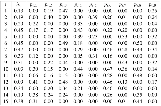
function. In the example, theλi are between 0 and 0.5, approximately 50% of thepi,j are equal to
zero indicating that taskjwill not find concerni, given that it is a fault, and the rest are between 0
and 0.5 and eachi is chosen to be 0.02. The values ofλiandpi,j used in the example are given in
Table 2.
4.2 Emulation
We wish to sequence the tasks in order to minimise the expected cost and time. We do so by
maximising the prior expected utility as outlined above. We have a single binary utility function
for cost and time. The conditional utilities used are those in (2). Suppose that initially the decision
maker felt that the utility of each was equally important. Thenq1= 1/2, q2= 1/2, q3= 0.
i λi pi,1 pi,2 pi,3 pi,4 pi,5 pi,6 pi,7 pi,8 pi,9
1 0.13 0.00 0.19 0.47 0.00 0.00 0.00 0.00 0.00 0.25
2 0.19 0.00 0.40 0.00 0.00 0.39 0.26 0.01 0.00 0.24
3 0.29 0.22 0.00 0.00 0.33 0.00 0.00 0.00 0.00 0.04
4 0.45 0.17 0.17 0.00 0.43 0.00 0.22 0.20 0.00 0.00
5 0.10 0.00 0.00 0.00 0.39 0.23 0.00 0.33 0.00 0.32
6 0.45 0.00 0.00 0.49 0.18 0.00 0.00 0.00 0.50 0.00
7 0.47 0.00 0.00 0.00 0.29 0.00 0.46 0.28 0.49 0.34
8 0.33 0.12 0.00 0.00 0.05 0.31 0.16 0.00 0.00 0.00
9 0.31 0.00 0.22 0.44 0.00 0.00 0.00 0.43 0.00 0.32
10 0.03 0.30 0.15 0.00 0.44 0.00 0.47 0.36 0.00 0.14
11 0.10 0.06 0.16 0.13 0.00 0.00 0.28 0.00 0.48 0.00
12 0.09 0.41 0.00 0.48 0.00 0.00 0.46 0.13 0.00 0.17
13 0.34 0.00 0.20 0.34 0.21 0.00 0.46 0.00 0.00 0.00
14 0.19 0.38 0.24 0.24 0.00 0.00 0.26 0.00 0.35 0.00
[image:16.612.138.474.70.292.2]15 0.38 0.31 0.00 0.00 0.00 0.00 0.00 0.01 0.44 0.00
Table 2: The values ofλiandpi,jused in the example.
takes 102 seconds in R version 3.3.1 on a machine with 16GB of RAM and an Intel Core
[email protected] GHz processor. If we increase the number of tasks this exhaustive search would take
around 17 minutes forJ = 10, 3.1 hours forJ = 11, 37 hours forJ = 12,20 days forJ = 13, 284 days forJ = 14 and 11.7 years forJ = 15.Thus, while we have chosen a number of tasks for which we can evaluate the success of the emulator by comparison with the exact solution in this
case, for moderately larger decision problems we would be unable to solve the problem exactly.
We suppose that we have a budget ofB = 100evaluations of the expected utility, which will be split betweenNevaluations at the training sample andMevaluations based on the topMsequences
under the emulator. In order to focus attention on the ability of the emulator, rather than the choice
of training sample, we choose the simplest possible design for our training sample, i.e.Nsequences
sampled uniformly from the set of allJ!sequences. With such a design, the empirical results of Section 5 suggest that the optimal split of our budget is approximatelyN = 60andM = 40, giving roughly a 75% chance of obtaining the optimal sequence. We use the Pearson correlation as our
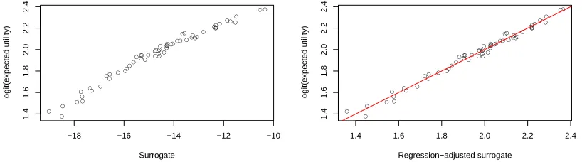
measure of correlationc(ψ), again due to its superior empirical performance; see Section 5. We first fit the initial surrogate based on the Benter model,fˆ(·), as described in Section 2.1. The opti-mal choice for this illustrative example isθˆ= (1.00,0.79,2.36,2.72,0.38,3.20,0.99,3.45,0.89)
of the association between the output under the surrogate and the logit expected utilities (to decide
if the association is likely to produce a good emulator). The values of the logit expected utility and
the surrogate function values at the 60 training points for this choice ofψare given in the left hand
side of Figure 1 and show a good correspondence.
● ● ● ● ● ● ● ● ● ● ● ● ● ● ● ● ● ● ● ● ● ● ● ● ● ● ● ● ● ● ● ● ● ● ● ● ● ● ● ● ● ● ● ● ● ● ● ● ● ● ● ● ● ● ●● ● ● ● ●
−18 −16 −14 −12 −10
1.4 1.6 1.8 2.0 2.2 2.4 Surrogate logit(e xpected utility) ● ● ● ● ● ● ● ● ● ● ● ● ● ● ● ● ● ● ● ● ● ● ● ● ● ● ● ● ● ● ● ● ● ● ● ● ● ● ● ● ● ● ● ● ● ● ● ● ● ● ● ● ● ● ●● ● ● ● ●
1.4 1.6 1.8 2.0 2.2 2.4
[image:17.612.97.506.181.295.2]1.4 1.6 1.8 2.0 2.2 2.4 Regression−adjusted surrogate logit(e xpected utility)
Figure 1: Logit transformed expected utilities versus surrogate function values for the training sample of sequences under the initial surrogatefˆ(·) (left) and the regression-adjusted surrogate
f?(·)(right).
Whilst the estimated parameters are largely a vehicle for obtaining an emulator, they do provide
some insight into the solution of the design problem. The rank order of theθˆk from largest to
smallest should be similar to the order of tasks with the highest value of the surrogate function: in
this case the order is(8,6,4,3,1,7,9,2,5), suggesting task 8 is performed first, followed by task 6 and so on. The relative values of theθˆkalso provide a rough guide to how persistent the tasks are
likely to be in the sequences with the highest values of the surrogate function; for example we can
see thatθˆ5 is much lower than the other parameters and so task 5 is likely to always be scheduled
last in the sequences with high values of the surrogate function. Similarly,αˆjcan be interpreted as
the importance of the task that is performedjth in the sequence. We see that the values forα1toα4
(and possiblyα5) are all relatively large and then the values start to tail off. This suggests that the
first four (or five) tasks may be the important tasks to schedule, perhaps due to the reliability target
being reached by then, with the last few not as important (in which case the order in which the tasks
are performed may have little impact on the expected utility).
We can evaluate the suitability of the regression-adjusted surrogate function; see Section 2.1.1.
In this case we obtainβb = (2.31,−0.07,−0.01,0.00)and this gives a sample correlation
functions, indicating that either would be a good emulator, however, in what follows we use the
regression-adjusted surrogate as that gave the higher Pearson correlation.
We evaluate the regression-adjusted surrogate function at all 9! sequences of tasks; this takes
approximately 17 seconds which is 6 times quicker than evaluating all of the expected utilities. For
increasing numbers of tasks the emulation would take around 3 minutes forJ = 10, 31 minutes for
J = 11, 6 hours 15 minutes forJ = 12, 3.4 days forJ = 13,47 days forJ = 14and 1.9 years for
J = 15. Each of these numbers represents a significant speed up over the exhaustive enumeration of the expected utility. However, even for moderateJ complete enumeration may be infeasible.
This potential drawback is easily addressed by the probabilistic nature of the surrogate model, as
[image:18.612.176.420.345.483.2]described in Section 5.4.
Figure 2 plots the logit transformed expected utility against the regression-adjusted surrogate
function for all 362,880 sequences.
1.2 1.4 1.6 1.8 2.0 2.2 2.4
1.2
1.6
2.0
2.4
Regression−adjusted surrogate
logit(e
xpected utility)
Figure 2: Logit transformed expected utilities versus regression-adjusted surrogate function values for all sequencesx; the colours indicate the first task in that sequence (1=black, 2=red, 3=green, 4=blue, 5=cyan, 6=magenta, 7=yellow, 8=grey, 9=purple).
The points in Figure 2 are colour-coded by the first task in each sequence. There is a clear
pos-itive relationship between the expected utilities and the surrogate output. The Pearson correlation
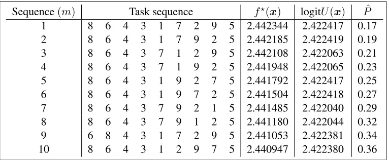
coefficient is 0.990. As there is not perfect correspondence betweenU(x)andf(x), we propose the remainingB−N = M = 40candidate sequences which have the highest values under the emulatorf?(·)and then evaluate the expected utility at theseM candidate values. In the interests of space, only the top ten sequences in terms of their values of the surrogate function are given in Table
Sequence(m) Task sequence f?(x) logitU(x) Pˆ
1 8 6 4 3 1 7 2 9 5 2.442344 2.422417 0.17
2 8 6 4 3 1 7 9 2 5 2.442185 2.422419 0.19
3 8 6 4 3 7 1 2 9 5 2.442108 2.422063 0.21
4 8 6 4 3 7 1 9 2 5 2.441948 2.422065 0.23
5 8 6 4 3 1 9 2 7 5 2.441792 2.422417 0.25
6 8 6 4 3 1 9 7 2 5 2.441504 2.422418 0.27
7 8 6 4 3 7 9 2 1 5 2.441485 2.422040 0.29
8 8 6 4 3 7 9 1 2 5 2.441180 2.422044 0.32
9 6 8 4 3 1 7 2 9 5 2.441053 2.422381 0.34
[image:19.612.115.498.71.229.2]10 8 6 4 3 1 2 9 7 5 2.440947 2.422380 0.36
Table 3: The ten sequences with the highest values off?(x)and their corresponding logit expected utilities. The final column gives an estimatePˆfor the probability that the optimal sequence is to be found in the topmsequences under the emulator for examples of this type.
not have the highest expected utility. Nevertheless, these top 10 sequences all have high expected
utility. The sequence which gives the maximum expected utility out of theB = N +M = 100
at which the expected utility was calculated, and is therefore our putative optimal sequence, is
˜
x= (8,6,4,3,1,7,9,2,5)which is ranked 2nd in terms of the emulator. Also in Table 3 we give an estimatePˆ for the probability that the optimal sequence is to be found in the topmsequences under the emulator for examples of this type. These estimates are based on a regression analysis of
the simulation results of Section 5.
As mentioned previously, we can evaluate all of the expected utilities for this example. The
sequences ranked by the highest expected utilities are given in Table 4. In practice, these sequences
would not typically be known. We show them here to investigate the ability of the surrogate function
to identify the globally optimal sequence.
The optimal sequence of tasks, that with the largest expected utility, isxˆ = (8,6,4,3,1,7,9,2,5). This matchesx˜, the putative optimal sequence which was highlighted in our candidate list. In this illustrative example, we have found the optimal sequence using onlyB = 100evaluations of the expensive expected utility. Our simulation results in Section 5 suggest that in similar examples,
with this choice ofN andMwe would obtain the optimal sequence roughly 75% of the time. Even
when we do not find the optimal sequence in theB evaluations, we still find sequences with close
to optimal values of the expected utility. For example, in this illustrative example, the sequence
with maximum value of the surrogate function has the 5th highest expected utility and matches the
Sequence Task sequence f†(x) U(x)
1 8 6 4 3 1 7 9 2 5 0.9199880 0.9185209
2 8 6 4 3 1 7 9 5 2 0.9197039 0.9185209
3 8 6 4 3 1 9 7 2 5 0.9199380 0.9185209
4 8 6 4 3 1 9 7 5 2 0.9196522 0.9185209
5 8 6 4 3 1 7 2 9 5 0.9199998 0.9185208
6 8 6 4 3 1 9 2 7 5 0.9199592 0.9185208
7 8 6 4 3 1 7 2 5 9 0.9196663 0.9185208
8 8 6 4 3 1 9 2 5 7 0.9195836 0.9185208
9 8 6 4 3 1 7 5 9 2 0.9197978 0.9185195
[image:20.612.135.474.71.227.2]10 8 6 4 3 1 7 5 2 9 0.9197485 0.9185195
Table 4: The ten sequences with the highest values ofU(x)and their corresponding values under
f†(·).
As illustrated above, in this example we have been able to evaluate the expected utility at all
pos-sible sequences of tasks and therefore been able to identify the optimal sequence, but our
method-ology is designed for scenarios where this is not possible. In such situations, a practitioner will
not know whether they have obtained the optimal sequence, or whether their putative optimal
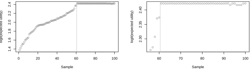
se-quence is close to the optimal. We therefore recommend a simple graphical diagnostic plot along
the lines of that in Figure 3. This compares graphically the logit transformed expected utilities in
●●
●●●
●●●
●●
●●●●
●●●
●●●●●●●
●●●●●●●
●●●●●●●●
●●●●●●●●●
●●●●
●●●●●
●
●●●●●●●●●●●●●●●●●●●●●●●●●●●●●●●●●●●●●●●●●●
0 20 40 60 80 100
1.4
1.6
1.8
2.0
2.2
2.4
Sample
logit(e
xpected utility)
● ●
● ● ●
● ● ● ● ● ● ● ● ● ● ● ● ● ● ● ● ● ● ● ● ● ● ● ● ● ● ● ● ● ● ● ●●● ●● ● ●● ●
60 70 80 90 100
2.30
2.35
2.40
Sample
logit(e
xpected utility)
Figure 3: Logit transformed expected utilities versus sample number. In each plot the points to the left of the vertical line represent the training samples (ordered by increasing expected utility) and the points to the right of the line correspond to theM sequences suggested by the emulator in decreasing order of the regression-adjusted surrogate function value. The left-hand plot shows all
B = 100 samples. The right-hand plot focuses on the top 5 from the training sample and theM
sequences proposed from the emulator.
the training sample of sizeN with those in the evaluation sample of sizeM. From such a plot, a
[image:20.612.100.500.433.546.2]expected utilities than those in the training sample and also the extent to which the expected utilities
of theM emulator-proposed sequences are all very similar. This is reassuring as it suggests that
the putative optimal sequence is probably close to optimal (in terms of the overall variation in logit
expected utilities that are observed in the training sample). So, whilst, in a real example, there are
no guarantees that the optimal sequence has been found, such a graphical diagnostic can provide
some reassurance that the putative optimal sequence is satisfactory.
As suggested by one of the referees, an alternative strategy for checking the stability of the
emulator and of the putative optimal sequence is to split the training sample into sub-samples and
perform the emulator fitting/exploration process on each sub-sample. Our experience, as reported
in the Supplementary Material, is that not much insight is gained by this splitting of the training
sample and so we have chosen not to pursue that procedure here.
4.3 Results
The optimal ordering of tasks has an expected utility of 0.919 and corresponds to the sequence
(8,6,4,3,1,7,9,2,5). That is, we first carry out task 8 and then if we haven’t met the reliability target we move on to task 6. If we still haven’t met the reliability target we then carry out task 4,
etc.
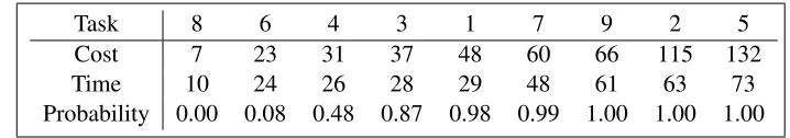
We consider the costs, times and probabilities of reaching the target reliability following each
task. They are given in Table 5.
Task 8 6 4 3 1 7 9 2 5
Cost 7 23 31 37 48 60 66 115 132
Time 10 24 26 28 29 48 61 63 73
[image:21.612.123.482.454.517.2]Probability 0.00 0.08 0.48 0.87 0.98 0.99 1.00 1.00 1.00
Table 5: Various quantities of interest broken down by task in the optimal sequence.
From the table we see that it is not likely that we will have to perform all of the tasks to achieve
the target reliability. It is likely that only 4 or 5 tasks will be needed and that we can reach the
reliability target with a spend of 37-48 and a time of 28-29. Note that this coincides with our
interpretation of theαparameters; the first 4 or 5 tasks have relatively large values ofαcompared
to the other tasks. We see that we are likely to spend a larger proportion of our total time than our
5
Simulation studies
5.1 Choice of surrogate model and correlation function
A simulation study was performed to assess the performance of several surrogate models based on
parametric probabilistic models for permutations: the Benter model (B) as described in Section 2.1;
the Plackett-Luce model (PL) which is obtained from the Benter model by settingα =1; and the reverse Plackett-Luce model (RPL) which is obtained via the PL model evaluated at the reverse
sequence of tasks. We did not include the regression-adjustment in the simulation study since it
can be applied to any surrogate function and will improve upon it. A range of correlation functions
(Pearson, Spearman and Kendall) were considered as the objective function for the fitting procedure
for each of the putative surrogate models. We have considered numbers of tasksJ ranging from 6
to 10 and three sets of trade-off parameters: (a)q1 = 1/2, q2 = 1/2, q3 = 0, (b)q1 = 1/3, q2 = 1/3, q3 = 1/3 and (c) q1 = 2/3, q2 = 2/3, q3 = −1/3. The problem set-up follows that in
Section 4 in which we seti = = 0.02, t = 100, R0 = 0.8, T0 = 90. To focus attention on
the performance of the emulator, rather than the effect that the design of the training samples has
on performance, we use the randomly sampled design strategy that was used for the illustrative
example in Section 4. In this way we separate the potential capability of each emulator from the
issue of training sample design.
For each combination of number of tasksJ, trade-off parametersq and initial random sample
sizeN, 100 sets of expected utilities for allJ!sequences were generated. For each of these 100 simulations we fitted each of the nine combinations of surrogate model and correlation function
based on the initial sample ofN sequences. We evaluated the surrogate function at allJ!possible sequences.
We focus on the results forJ = 9tasks and trade-off parameters (b); the differences for the other combinations of trade-off parameters were minimal and other values ofJ from 6 to 10 gave
broadly similar results, though the differences between the performance of the surrogate models
and correlation functions increase asJ increases.
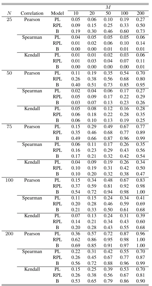
Table 6 shows the estimated probability that the optimal sequence in terms of expected utility
is contained in either theN initial sequences or the further M sequences based on the best M
sequences in terms of the surrogate function, for a range of values ofN andM.
M
[image:23.612.184.427.67.524.2]N Correlation Model 10 20 50 100 200 25 Pearson PL 0.05 0.06 0.10 0.19 0.27 RPL 0.09 0.15 0.25 0.33 0.50 B 0.19 0.30 0.46 0.60 0.73 Spearman PL 0.04 0.05 0.05 0.05 0.06 RPL 0.01 0.02 0.06 0.10 0.14 B 0.00 0.00 0.01 0.01 0.01 Kendall PL 0.01 0.01 0.02 0.03 0.06 RPL 0.01 0.03 0.04 0.07 0.11 B 0.00 0.00 0.00 0.00 0.01 50 Pearson PL 0.11 0.19 0.35 0.54 0.70 RPL 0.26 0.38 0.56 0.68 0.80 B 0.40 0.51 0.73 0.85 0.95 Spearman PL 0.02 0.04 0.06 0.17 0.27 RPL 0.05 0.09 0.17 0.22 0.29 B 0.03 0.07 0.13 0.23 0.26 Kendall PL 0.05 0.08 0.12 0.16 0.28 RPL 0.06 0.18 0.22 0.28 0.35 B 0.06 0.10 0.13 0.19 0.25 75 Pearson PL 0.15 0.29 0.49 0.67 0.77 RPL 0.35 0.46 0.68 0.77 0.89 B 0.49 0.66 0.87 0.96 0.99 Spearman PL 0.06 0.11 0.17 0.26 0.35 RPL 0.16 0.23 0.29 0.43 0.56 B 0.17 0.21 0.32 0.42 0.54 Kendall PL 0.04 0.09 0.19 0.26 0.34 RPL 0.10 0.19 0.31 0.42 0.50 B 0.10 0.20 0.32 0.38 0.47 100 Pearson PL 0.15 0.34 0.48 0.67 0.83 RPL 0.37 0.59 0.81 0.92 0.98 B 0.54 0.72 0.94 0.98 1.00 Spearman PL 0.11 0.15 0.24 0.34 0.41 RPL 0.20 0.28 0.46 0.59 0.69 B 0.21 0.33 0.50 0.61 0.68 Kendall PL 0.07 0.13 0.24 0.31 0.39 RPL 0.14 0.21 0.34 0.43 0.60 B 0.20 0.28 0.43 0.55 0.68 200 Pearson PL 0.36 0.57 0.72 0.87 0.96 RPL 0.62 0.86 0.95 0.98 1.00 B 0.69 0.85 0.91 0.97 1.00 Spearman PL 0.22 0.31 0.42 0.55 0.70 RPL 0.26 0.45 0.67 0.77 0.87 B 0.56 0.72 0.88 0.96 0.99 Kendall PL 0.15 0.25 0.39 0.53 0.70 RPL 0.26 0.38 0.56 0.67 0.81 B 0.53 0.65 0.79 0.86 0.90
Table 6: Estimated probability from 100 simulations that the optimal sequence is found in an ini-tial random sample ofN sequences followed by the top M sequences under various surrogates: PL=Plackett-Luce, RPL=Reverse Plackett-Luce, B=Benter.
better than using the other two correlation functions. Within the results for the Pearson correlation,
the surrogate based on the Benter model (fˆ(·)), is almost uniformly better than the other two models (PL and RPL), and provides a noticeable improvement for smallN andM. The results justify our
preference for the Benter model over the PL or RPL models as the basis for a parametric surrogate.
Benter and Pearson.
5.2 Guidelines on choice ofN for a given budgetB
Table 6 provides some guidelines on the choices ofN andM for problems such as this, which
are useful if we have a specific budget of B = N +M sequences for which we can calculate the expected utility. For example, with a budget ofB = 150 sequences, the probability that we obtain the optimal sequence is approximately 85% whenN = 50, M = 100, whereas withN = 100, M = 50this probability is approximately 94%.
The results in Table 6 relate to one specific “problem scenario” as defined through the values
ofJ, I, R0, , λ, p, q and so on, and are perhaps too narrowly focused to provide generic advice.
A more extensive simulation study was carried out in order to offer more generic guidance on the
choice ofN for a givenB, over a broad range of “problem scenarios”. A total of 10000 randomly
generated “problem scenarios” were analysed in the second simulation study and the results are
described in detail in the Supplementary Material. Specifically, we fit a logistic regression model
with response variable an indicator of whether the optimal sequence was found for that problem
scenario and with explanatory variables equal toN,B and functions thereof. This approach allows
us to predict the probability of finding the optimal sequence for combinations of N and B, to
approximate the optimal choice ofN for a given budgetBand predict the probability of obtaining
the optimal sequence for that choice. Based on the results of this second simulation study we would
recommend therule of thumb of setting N = M, or, in other words, settingN = B/2 (to the nearest integer). This provides a simple, default first choice in the absence of other information.
Our simulations suggest that this is only marginally suboptimal, as well as being very simple and
easy to remember.
Additionally, we have used the simulation results from Table 6 to determine an optimal choice
ofN for a given budgetB for the specific “problem scenario” considered therein. Specifically,
fol-lowing the logistic regression procedure outlined in the Supplementary Material, the results suggest
that, ifB = 100, which was used in the illustrative example of Section 4, the optimal choice ofN
is 58 (and thereforeM = 42); this gives a probability of obtaining the optimal sequence of about
N andM and a probability of obtaining the optimal sequence of just over70%(as determined by the results in the Supplememtary Material).
5.3 Median rank performance
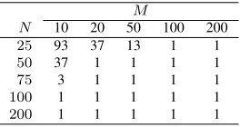
Whilst we may not obtain the optimal sequence in ourN+M sequences it is interesting to know how the best ranked sequence in our sample compares to the full set of sequences. In each of our
simulations in the first simulation study (detailed in Section 5.1) we computed the rank in terms of
expected utilities of the highest ranked sequence out of our sample ofN +M sequences for the values ofN andM. The medians over 100 simulations of these ranks are given in Table 7. We
M
[image:25.612.239.371.273.343.2]N 10 20 50 100 200 25 93 37 13 1 1 50 37 1 1 1 1 75 3 1 1 1 1 100 1 1 1 1 1 200 1 1 1 1 1
Table 7: Median from 100 simulations of the rank in terms of expected utilities of the highest ranked sequence out of our sample ofB =N +M sequences for the emulator based on the Benter model with maximised Pearson correlation.
see that even in very small sample sizes we do well at choosing a good sequence, and for most
combinations ofN andM we get the optimal sequence at least 50% of the time.
5.4 Dealing with large numbers of permutations
In our examples and simulation studies we have considered a fairly small number of tasks (up to
J = 10) so that we could evaluate the expected utility for allJ!sequences and solve the decision problem exactly. This also means that we were able to evaluate the surrogate function at all possible
sequences and find the topM candidates for evaluating the expected utility. If we were interested
in sequencing a larger number of tasks, sayJ = 20, it may be infeasible to evaluate the surrogate function at allJ!sequences. One advantage of an emulator based on a probabilistic model is that we can sample a large number of sequences (though considerably less thatJ!) from the fitted Benter model, evaluate the surrogate function at these values, and then pick the topMas the candidates to
evaluate the expected utility. This simulation-based approach should scale up well to very largeJ,
6
Summary and further work
We have considered the emulation of utility functions for permutations. We proposed an approach
based on the Benter model and have shown this can provide a good approximation in reliability
growth decision making. A simple extension would be to consider the case where some tasks can
be carried out in parallel.
Our proposed emulator is a unimodal function of its inputs. In the illustrative example of
Sec-tion 4 the utility funcSec-tion was unimodal, and for the types of reliability growth tasks we consider
here we expect the utility function to be largely unimodal, and so our proposed emulator is
ide-ally suited. More generide-ally, for mutli-modal utility functions, our proposed emulator will emulate
around only one of the modes. As such, the development of a multi-modal surrogate based on a
mixture of Benter models [Gormley and Murphy, 2008, Mollica and Tardella, 2014] may be worth
investigating.
We chose the training set of N sequences randomly. Future work would be to choose this
training sample informatively, to focus the training sample in the areas of high expected utility. The
ratio of benefit to cost of tasks would be useful here. The approach taken for reliability growth,
maximising the expected utility of a multi-attribute utility function, can have wider use in problems
in which actions are to be ordered. A future direction is to use the approach in optimal sequencing
of actions in project risk management.
We emphasise that the results presented in Sections 4 and 5 are based on a simple random
sam-ple from the set of all sequences and that other more intelligent ways to explore the design space
may lead to different results in terms of optimal choices ofN andM. Nevertheless this procedure
allows us to assess the performance of the different surrogates and we suspect that the main
mes-sages from our simulation study — that the Benter model is preferred to the PL or RPL models, and
the Pearson correlation is the superior form of objective function — will persist with other types of
training sample. This has been our experience in some preliminary investigations. Our proposed
procedure has similarities to an efficient single-step cross-entropy optimization algorithm
[Rubin-stein and Kroese, 2004]. Simulation results (given in the Supplementary Material) using a training
sample derived from two steps of the cross-entropy optimization algorithm (that is, with training
presented here. The results in terms of the probability of discovering the optimal sequence in the
N +M sequences are no better than those presented here for large values ofN andM, and are typically poorer for small values ofN andM. A more detailed investigation of design issues is the
subject of future work.
References
W. Benter. Computer-based horse race handicapping and wagering systems: A report. In D.B. Hausch, V.S.Y. Lo, and
W.T. Ziemba, editors,Efficiency of Racetrack Betting Markets, pages 183–198. Academic Press, San Diego, 1994.
W.R. Blischke and D.N.P Murthy.Reliability: Modeling, Prediction, and Optimization. Wiley Series in Probability and
Statistics. Wiley, 2011. ISBN 9781118150474.
M. Caserta and S. Voß. An exact algorithm for the reliability redundancy allocation problem. European Journal of
Operational Research, 244(1):110–116, 2015.
L.H. Crow.Reliability analysis of complex repairable systems. SIAM, 1974.
A.P. Eigbe, B.J. Sauser, and W. Felder. Systemic analysis of the critical dimensions of project management that impact
test and evaluation program outcomes.International Journal of Project Management, 33(4):747–759, 2015.
M.A. Fligner and J.S. Verducci. Multistage ranking models.Journal of the American Statistical Association, 83:892–901,
1988.
I.C. Gormley and T.B. Murphy. Exploring voting blocs within the Irish electorate: a mixture modeling approach.Journal
of the American Statistical Association, 103:1014–1027, 2008.
S. Guikema and M.E. Pate-Cornell. Component choice for managing risk in engineered systems with generalized
risk/cost functions.Reliability Engineering and System Safety, 78:227–238, 2002.
D.A. Henderson, R.J. Boys, K.J. Krishnan, C. Lawless, and D.J. Wilkinson. Bayesian emulation and calibration of
a stochastic computer model of mitochondrial dna deletions in substantia nigra neurons. Journal of the American
Statistical Association, 104:76–87, 2009.
C. Hsieh. Optimal task allocation and hardware redundancy policies in distributed computing systems.European Journal
of Operational Research, 147:430–447, 2003.
C. Hsieh and Y. Hsieh. Reliability and cost optimization in distribution computing systems.Computers and Operations
Research, 30:1103–1119, 2003.
W. Johnston, J. Quigley, and L. Walls. Optimal allocation of reliability tasks to mitigate faults during system development.
IMA Journal of Management Mathematics, 17:159–169, 2006.
D.R. Jones, M. Schonlau, and W.J. Welch. Efficient global optimization of expensive black-box functions. Journal of
Global Optimization, 13:455–492, 1998.
M. Kennedy and A. O’Hagan. Bayesian calibration of computer models (with discussion).J. R. Statist. Soc. Ser. B, 63:
425–464, 2001.
Y.H. Kim, A. Moraglio, A. Kattan, and Y. Yoon. Geometric generalisation of surrogate model-based optimisation to
combinatorial and program spaces.Mathematical Problems in Engineering, 2014, 2014.
K. Knight.Mathematical Statistics. Chapman and Hall, 2000.
M. Krasich. Modeling of sw reliability in early design with planning and measurement of its reliability growth. In
Reliability and Maintainability Symposium (RAMS), 2015 Annual, pages 1–6. IEEE, 2015.
M. Krasich, J. Quigley, and L. Walls. Modeling reliability growth in the product design process. InReliability And
Maintainability, 2004 Annual Symposium-RAMS, pages 424–430. IEEE, 2004.
G. Levitin, L. Xing, S. Peng, and Y. Dai. Optimal choice of standby modes in 1-out-of-n system with respect to mission
reliability and cost.Applied Mathematics and Computation, 258:587–596, 2015.
R.D. Luce.Individual Choice Behavior. Wiley, New York, 1959.
J.I. Marden.Analysing and Modeling rank data. Chapman and Hall, London, 1995.
C. Mollica and L. Tardella. Epitope profiling via mixture modelling of ranked data.Statistics in Medicine, 33:3738–3758,
2014.
A. Moraglio and A. Kattan. Geometric generalisation of surrogate model-based optimisation to combinatorial spaces. In
Evolutionary Computation in Combinatorial Optimization, pages 142–154. Springer, 2011.
A. Moraglio, Y.H. Kim, and Y. Yoon. Geometric surrogate-based optimisation for permutation-based problems. In
Proceedings of the 13th Annual Conference Companion on Geometric and Evolutionary Computation, pages 133– 134. ACM, 2011.
P. M¨uller and G. Parmigiani. Optimal design via curbe fitting of Monte Carlo experiments. Journal of the American
J.A. Nelder and R. Mead. A simplex method for function minimization.Computer Journal, 7:308–313, 1965.
P.D.T. O’Connor and A. Kleyner.Practical reliability engineering. John Wiley & Sons, 2012.
R. L. Plackett. The analysis of permutations.Applied Statistics, 24:193–202, 1975.
J. Quigley and L. Walls. Measuring the effectiveness of reliability growth testing.Quality and Reliability Engineering,
15:87–93, 1999.
J. Quigley and L. Walls. Confidence intervals for reliability growth models with small sample sizes.IEEE Transactions
on Reliability, 52:257–262, 2003.
J. Quigley and L. Walls. Trading reliability targets within a supply chain using Shapley’s value.Reliability Engineering
and System Safety, 92:1448–1457, 2006.
R Core Team. R: A Language and Environment for Statistical Computing. R Foundation for Statistical Computing,
Vienna, Austria, 2014.
R.Y. Rubinstein and D.P. Kroese. The Cross-Entropy Method: A Unified Approach to Combinatorial Optimization,
Monte-Carlo Simulation, and Machine Learning. Springer-Verlag, New York, 2004.
J. Sacks, W.J. Welch, T.J. Mitchell, and H.P. Wynn. Design and analysis of computer experiments. Statistical Science,
4:409–423, 1989.
M. Silverman. Summary of halt and hass results at an accelerated reliability test center. InReliability and Maintainability
Symposium, 1998. Proceedings., Annual. IEEE,, 1998.
U.S. Department of Defense. Defense science board task force report on developmental test and evaluation. Technical report, 2008.
U.S. Department of Defense. Directive-type memorandum (dtm) 11-003 - reliability analysis, planning, tracking, and reporting. Technical report, 2011.
I. Voutchkov, A.J. Keane, A. Bhaskar, and T.M. Olsen. Weld sequence optimization: The use of surrogate models for
solving combinatorial problems. Computational Methods in Applied Mechanics and Engineering, 194:3535–3551,
2005.
L. Walls and J. Quigley. Learning to improve reliability during system development. European Journal of Operational
Research, 119:495–509, 1999.
L. Walls and J. Quigley. Building prior distributions to support bayesian reliability growth modelling using expert
judgement.Reliability Engineering and System Safety, 74:117–128, 2001.
L. Walls, J. Quigley, and M. Kraisch. Comparison of two models for managing reliability growth during product
devel-opment.IMA Journal of Mathematics Applied in Business and Industry, 16:12–22, 2005.
M. Wayne and M. Modarres. A bayesian model for complex system reliability growth under arbitrary corrective actions.
Reliability, IEEE Transactions on, 64(1):206–220, 2015.
K.J. Wilson and J. Quigley. Allocation of tasks for reliability growth using multi-attribute utility. European Journal of
Operational Research, 255:259–271, 2016.
P.C. Young and M. Ratto. Statistical emulation of large linear dynamic models.Technometrics, 53(1):29–43, 2011.
M. Zaefferer. Package ‘CEGO’.https://cran.r-project.org/web/packages/CEGO/CEGO.pdf, 2015.
M. Zaefferer, J. Stork, and T. Bartz-Beielstein. Distance measures for permutations in combinatorial efficient global
optimization. InParallel Problem Solving from Nature - PPSN XIII, volume 8672 ofLecture Notes in Computer
Science, pages 373–383. Springer, 2014a.
M. Zaefferer, J. Stork, M. Friese, A. Fischbach, B. Naujoks, and T. Bartz-Beielstein. Efficient global optimization for
combinatorial problems. InProceedings of the 2014 Annual Conference on Genetic and Evolutionary Computation,
pages 871–878. ACM, 2014b.
Q. Zhou, P.Z.G. Qian, and S. Zhou. A simple approach to emulation for computer models with qualitative and quantitative