Estimation of a regression spline sample selection model

City, University of London Institutional Repository

Citation

:

Marra, G and Radice, R. ORCID: 0000-0002-6316-3961 (2013). Estimation of a

regression spline sample selection model. Computational Statistics & Data Analysis, 61, pp.

158-173. doi: 10.1016/j.csda.2012.12.010

This is the published version of the paper.

This version of the publication may differ from the final published

version.

Permanent repository link:

http://openaccess.city.ac.uk/20950/

Link to published version

:

http://dx.doi.org/10.1016/j.csda.2012.12.010

Copyright and reuse:

City Research Online aims to make research

outputs of City, University of London available to a wider audience.

Copyright and Moral Rights remain with the author(s) and/or copyright

holders. URLs from City Research Online may be freely distributed and

linked to.

Contents lists available atSciVerse ScienceDirect

Computational Statistics and Data Analysis

journal homepage:www.elsevier.com/locate/csda

Estimation of a regression spline sample selection model

Giampiero Marra

a,∗

, Rosalba Radice

b

a_{Department of Statistical Science, University College London, London WC1E 6BT, UK}

b_{Department of Economics, Mathematics and Statistics, Birkbeck, University of London, London WC1E 7HX, UK}

a r t i c l e i n f o

Article history:

Received 23 July 2012

Received in revised form 15 December 2012 Accepted 15 December 2012

Available online 23 December 2012

Keywords:

Non-random sample selection Penalized regression spline Selection bias

Simultaneous equation system

a b s t r a c t

It is often the case that an outcome of interest is observed for a restricted non-randomly selected sample of the population. In such a situation, standard statistical analysis yields biased results. This issue can be addressed using sample selection models which are based on the estimation of two regressions: a binary selection equation determining whether a particular statistical unit will be available in the outcome equation. Classic sample selection models assume a priori that continuous regressors have a pre-specified linear or non-linear relationship to the outcome, which can lead to erroneous conclusions. In the case of continuous response, methods in which covariate effects are modeled flexibly have been previously proposed, the most recent being based on a Bayesian Markov chain Monte Carlo approach. A frequentist counterpart which has the advantage of being computationally fast is introduced. The proposed algorithm is based on the penalized likelihood estimation framework. The construction of confidence intervals is also discussed. The empirical properties of the existing and proposed methods are studied through a simulation study. The approaches are finally illustrated by analyzing data from the RAND Health Insurance Experiment on annual health expenditures.

©2012 Elsevier B.V.

1. Introduction

Sample selection models are used when the observations available for statistical analysis are not from a random sample of the population. Instead, individuals may have selected themselves into (or out of) the sample based on a combination of observed and unobserved characteristics. The use of statistical models ignoring such a non-random selection can have severe detrimental effects on parameter estimation.

As a motivating example, consider the RAND Health Insurance Experiment (RHIE), a study conducted in the United States between 1974 and 1982 (Newhouse, 1999). The aim was to quantify the relationship between various demographic and socio-economic characteristics (seeTable 6in Section4) and annual health expenditures in the population as a whole. Non-random selection arises if the sample consisting of individuals who used health care services differ in important characteristics from the sample of individuals who did not use them. When the relationship between the decision to use the services and health expenditure is through observables, selection bias can be avoided by accounting for these variables. However, if some individuals are part of the selected subsample because of some observables as well as unobservables, then regardless of whether such variables are correlated in the population they will be in the selected sample (e.g.,Dubin and Rivers, 1990). Hence, the neglect of this potential correlation can lead to inconsistent estimates of the covariate effects in the equation for annual expenditure.

Statistical methods correcting for the bias induced by non-random sample selection involve the estimation of two regression models: the selection equation (e.g., decision to use health services), and outcome equation (e.g., amount of health

∗_{Corresponding author. Tel.: +44 0 20 7679 1864; fax: +44 0 20 3108 3105.}

E-mail addresses:[email protected](G. Marra),[email protected](R. Radice). 0167-9473©2012 Elsevier B.V.

doi:10.1016/j.csda.2012.12.010

Open access under CC BY license.

care expenditure). The latter is used to examine the substantive question of interest, whereas the former is used to detect selection bias and obtain consistent estimates of the covariate effects in the outcome equation. Since their introduction by

Heckman(1979), sample selection models have been used in various fields (e.g.,Bärnighausen et al.,2011;Cuddeback et al.,

2004;Montmarquette et al.,2001;Sigelman and Zeng, 1999;Winship and Mare, 1992). Most of the case studies consider parametric sample selection models where continuous predictors have a pre-specified linear or non-linear relationship to the response variable. The need for techniques modeling flexibly regressor effects, without making a priori assumptions, arises from the observation that all parameter estimates are inconsistent when the relationship between covariates and outcome is mismodeled (e.g.,Chib et al.,2009;Marra and Radice, 2011). This may prevent the researcher from recognizing, for instance, strong covariate effects or revealing interesting relationships. Going back to the health expenditure example, covariates such as age and education are likely to have a non-linear relationship to both decision to use health services and amount to spend on them. Imposing a priori a linear relationship (or non-linear by simply using quadratic polynomials, for example) could mean failing to capture possibly important complex relationships.

In a parametric context, sample selection models are typically estimated using the two-step framework first introduced byHeckman(1979): using the parameter estimates of the selection equation, a component (called inverse Mills ratio) is calculated and then included in the outcome equation to correct for non-random sample selection. Such an approach was proposed to deal with violations of the assumption of normality. However, it has been found to be sensitive to correlation among covariates in the outcome and selection equations, which can be really problematic in applications (Puhani, 2000). This problem can be alleviated by imposing an exclusion restriction, which requires at least one extra covariate to be a valid predictor in the selection equation but the outcome equation. A number of estimation methods which do not impose parametric forms on the error distribution have been introduced. These are termed ‘semiparametric’ since only part of the model of interest (the linear predictor) is parametrically pre-specified (e.g.,Ahn and Powell, 1993;Lee,1994;Martins,

2001;Newey et al.,1990;Powell,1994;Vella,1998). In this direction, recent developments includeMarchenko and Genton

(2012) andvan Hasselt(2011). The sample selection literature has also been focusing on models with non-normal responses (e.g.,Boyes et al.,1989;Terza,1998;Smith,2003;Greene,2012). There are other variants of the sample selection model; these includeLi(2011) who considered the case in which there is more than one selection mechanism, andOmori and Miyawaki(2010) who extended selection models to allow threshold values to depend on individuals’ characteristics. These models have also been compared to principal stratification in the context of causal inference with nonignorable missingness (Mealli and Pacini, 2008).

We are interested in modeling flexibly covariate effects when the response is Gaussian.Das et al.(2003) considered the estimation of non-linear effects by extending theHeckman(1979) two-step estimation procedure. Recently,Chib et al.

(2009) andWiesenfarth and Kneib(2010) have introduced two more general estimation methods. Specifically, the approach of the former authors is based on Markov chain Monte Carlo simulation techniques and uses a simultaneous equation system that incorporates Bayesian versions of penalized smoothing splines. The latter further extended this approach by introducing a Bayesian algorithm based on low rank penalized B-splines for non-linear effects, varying-coefficient terms and Markov random-field priors for spatial effects. Using a model specification that is very similar to that ofWiesenfarth and Kneib(2010), we introduce a frequentist counterpart which has the advantage of being computationally fast. Our proposal can especially appeal to practitioners already familiar with traditional frequentist techniques. The proposed algorithm is based on the penalized maximum likelihood (ML) estimation framework, and is implemented in the

R

package

SemiParSampleSel

(Marra and Radice, 2012). As in a Bayesian framework, the proposal supports the choice of any class of smoothers albeit without requiring extra computational effort, an advantage which is not shared by a Bayesian implementation. The construction of confidence intervals is also discussed. The performance of the proposed and available methods are examined through a simulation study. Finally, the methods are illustrated analyzing data from the RAND Health Insurance Experiment on annual health expenditures.

2. Regression spline sample selection model

2.1. Model structure

The model consists of a system of two equations. Using the latent variable representation, the selection equation is

y∗_1i

=

uT_1i

θ

1

+

K1



k1=1

s1k1

(

z1k1i

)

+

ε

1i

,

i

=

1

, . . . ,

n

,

(1)

wherenis the sample size, andy∗

1iis a latent continuous variable which determines its observable counterparty1ithrough the rule 1

(

y∗

1i

>

0

)

. The outcome equation determining the response variable of interest is

y2i

=











uT_2i

θ

2

+

K2



k2=1

s2k2

(

z2k2i

)

+

ε

2i ify ∗ 1i

>

0

not observed ify∗_1i

≤

0

.

VectoruT 1i

=



1

,

u12i

, . . . ,

u1P1i



is theith row ofU₁

=



uT 11

, . . . ,

u

T 1n



T

, then

×

P1model matrix containingP1parametric model components (such as the intercept, dummy and categorical variables), with corresponding parameter vector

θ

1, and thes1k1 are unknown smooth functions of theK1continuous covariatesz1k1i. In line withWiesenfarth and Kneib(2010),

our implementation also supports varying coefficients models, obtained by multiplying one or more smooth terms by some predictor(s) (Hastie and Tibshirani, 1993), and smooth functions of two or more (e.g., spatial) covariates as described in Wood(2006,pp. 154–167). Similarly, uT

2i

=



1

,

u22i

, . . . ,

u2P2i



is theith row vector of thens

×

P2 model matrix

U2

=



uT 21

, . . . ,

u

T 2ns



T

, with coefficient vector

θ

2, and thes2k2are unknown smooth terms of theK2continuous regressors z2k2i.nsdenotes the size of the selected sample. For identification purposes, the smooth functions are subject to the centering

constraint



isk

(

zki

)

=

0 (Wood, 2006). As inChib et al.(2009) andWiesenfarth and Kneib(2010), we make the assumption that unobserved confounders have a linear impact on the responses. That is, the errors

(ε

1i

, ε

2i

)

are assumed to follow the bivariate distribution



ε

1i

ε

2i



i.i.d.

∼

N



0 0



,



1

ρσ

2

ρσ

2

σ

22



,

(3)

where

ρ

is the correlation coefficient,

σ

2the standard deviation of

ε

2iand

σ

1, the standard deviation of

ε

1i, is set to 1 because the parameters in the selection equation can only be identified up to a scale coefficient (e.g.,Greene, 2012, p. 686). The assumption of normality may be, perhaps, too restrictive for applied work; however it is typically made to obtain more tractable expressions.

The smooth functions are represented using the regression spline approach. To fix ideas and in the one-dimensional case, a genericsk

(

zki

)

is approximated by a linear combination of known spline basis functions,bkj

(

zki

)

, and regression parameters,

β

kj,

sk

(

zki

)

=

Jk



j=1

β

kjbkj

(

zki

)

=

Bk

(

zki

)

T

β

k

,

whereJkis the number of spline bases (hence regression coefficients) used to representsk

,

Bk

(

zki

)

T is theith vector of dimensionJkcontaining the basis functions evaluated at the observationzki, i.e.Bk

(

zki

)

=



bk1

(

zki

),

bk2

(

zki

), . . . ,

bkJk

(

zki

)



T , and

β

_kthe corresponding parameter vector. CalculatingBk

(

zki

)

for eachiyieldsJkcurves (encompassing different degrees of complexity) which multiplied by some real valued parameter vector

β

_kand then summed will give a (linear or non-linear) estimate forsk

(

zk

)

. The number of basis functions,Jk, determines the flexibility allowed forsk

(

zk

)

;

Jk

=

10 will lead to a ‘‘wigglier’’ curve estimate than when such a parameter is set to 5, for instance. Because, in practice, it is not easy to determine the optimal number of basis functions for thesk

(

zki

)

, a reasonably large number for theJkis typically chosen (to allow enough flexibility in the model) and then the corresponding

β

_kpenalized in order to suppress that part of non-linearity which is not supported from the data. As it will be shown in the next section, this can be achieved using a penalized estimation approach which is the mainstream in the regression spline literature (seeRuppert et al., 2003andWood, 2006for more details). Basis functions should be chosen to have convenient mathematical properties and good numerical stability. Many choices are possible and supported in our implementation including B-splines, cubic regression and low rank thin plate regression splines (e.g.,Ruppert et al., 2003). The case of smooths of more than one variable follows a similar construction. Based on the result above, Eqs.(1)and(2)can be written as

y∗_1i

=

uT

1i

θ

1

+

BT1i

β

1

+

ε

1i

,

i

=

1

, . . . ,

n

,

(4)

and

y2i

=

uT2i

θ

2

+

BT2i

β

2

+

ε

2i

,

i

=

1

, . . . ,

ns

,

(5)

whereBT

vi

=



B_v1

(

zv1i

)

T

, . . . ,

BvKv

(

zvKvi

)

T



and

β

T_v

=

(

β

T_v1

, . . . ,

β

T_vK

v

)

, for

v

=

1

,

2.

In principle, the parameters of the sample selection model are identified even if



uT 1i

,

B

T 1i



=



uT 2i

,

B

T 2i



(Wiesenfarth and Kneib, 2010). In practice, however, the absence of equation-specific regressors may lead to a likelihood function which does not vary significantly over a wide region around the mode (e.g.,Marra and Radice, 2011). Moreover, in applications, both functional form and model errors are likely to be misspecified to some degree. This suggests that empirical identification is better achieved if an exclusion restriction (ER) on the covariates in the two equations holds (e.g.,Chib et al.,2009;Vella,

1998). That is, the regressors in the selection equation should contain at least one or more regressors not included in the outcome equation. See the simulation results in Section3for more discussion of this issue.

2.2. A penalized maximum likelihood estimation approach

Recall that the error terms

(ε

1i

, ε

2i

)

are assumed to follow a bivariate normal distribution and define the linear predictors

η

vi

=

uT_vi

θ

v

+

B

T

group of observations has a different form for the likelihood. Wheny2iis observed, the likelihood function is the probability of the joint eventy2iandy∗1i

>

0, i.e.

P

(

y2i

,

y

∗

1i

>

0

)

=

f

(

y2i

)

P



y∗1i

>

0

|

y2i



=

f

(ε

2i

)

P

(ε

1i

>

−

η

1i

|

ε

2i

)

=

1

σ

2

φ



y2i

−

η

2i

σ

2

 

∞ −η1i

f

(ε

1i

|

ε

2i

)

d

ε

1i

=

1

σ

2

φ



y2i

−

η

2i

σ

2

 

∞ −η1i

1



1

−

ρ

2

φ



ε

1i

−

_σρ₂

(

y2i

−

η

2i

)



1

−

ρ

2



d

ε

1i

=

1

σ

2

φ



y2i

−

η

2i

σ

2



Φ



η

1i

+

_σρ₂

(

y2i

−

η

2i

)



1

−

ρ

2



.

Wheny2iis not observed, the likelihood function just corresponds to the marginal probability thaty∗1i

≤

0, i.e.

P



y∗1i

≤

0



=

_P

(ε

_1i

≤ −

η

_1i

)

=

Φ

(

−

η

_1i

)

=

1

−

Φ

(η

_1i

) .

Therefore, the log-likelihood function for the complete sample of observations is

ℓ(

δ

)

=

n



i=1

(

1

−

y1i

)

log

{

1

−

Φ

(η

1i

)

} +

y1i



−

log

σ

2

+

log

φ



y2i

−

η

2i

σ

2



+

logΦ



η

1i

+

_σρ₂

(

y2i

−

η

2i

)



1

−

ρ

2



,

where

δ

T

₌

₍

_δ

T 1

,

δ

T

2

, σ

2

, ρ)

and

δ

T_v

=

(

θ

_vT

,

β

T_v

)

, for

v

=

1

,

2.

As explained in the previous section, because of the flexible linear predictor structure considered in this article, unpenalized ML estimation is likely to result in smooth term estimates which are too rough to produce practically useful results. This issue can be dealt with by augmenting the objective function with a penalty term, such as



2

v=1



Kv

kv=1

λ

vkv



s′′_k

(

z_vkv

)

2dzvkv, measuring the (second-order, in this case) roughness of the smooth terms in the model.

The

λ

_vkv are smoothing parameters controlling the trade-off between fit and smoothness. Since regression splines are

linear in their model parameters, such a penalty can be expressed as a quadratic form in

β

T

=

(

β

T₁

,

β

T₂

)

, i.e.

β

TS_λ

β

where

S_λ

=



2

v=1



Kv

kv=1

λ

vkvSvkv and theSvkvare positive semi-definite known square matrices. The penalized log-likelihood is

therefore given as

ℓ

p

(

δ

)

=

ℓ(

δ

)

−

1 2

β

T

S_λ

β

.

(6)

Because

ρ

is bounded in

[−

1

,

1

]

and

σ

2 can only take positive real values, we use

ρ

∗

=

tanh−1

(ρ)

=

(

1

/

2

)

log

{

(

1

+

ρ) / (

1

−

ρ)

}

and

σ

₂∗

=

log

(σ

2

)

in optimization. Given values for the

λ

vkv, we seek to maximize(6). In

practice, this can be achieved by Newton–Raphson’s methods iterating

ˆ

δ

[a+1]

= ˆ

δ

[a]

+

(

H[a]

−

S_λ∗

)

−1

(

S∗_λ

δ

ˆ

[a]

−

g[a]

)

(7)

until convergence, whereais an iteration index andS∗

λan overall block-diagonal penalty matrix, i.e.

S∗_λ

=

diag

(

011

, . . . ,

01P1

, λ

1k1S1k1

, . . . , λ

1K1S1K1

,

021

, . . . ,

02P2

, λ

2k2S2k2

, . . . , λ

2K2S2K2

,

0

,

0

).

The score vectorgis defined by two subvectorsg₁

=

∂ℓ(

δ

)/∂

δ

₁andg₂

=

∂ℓ(

δ

)/∂

δ

₂and two scalarsg3

=

∂ℓ(

δ

)/∂σ

2∗ and g4

=

∂ℓ(

δ

)/∂ρ

∗, while the Hessian matrix has a 4

×

4 matrix block structure with

(

r

,

h

)

th element Hr,h

=

∂

2

_ℓ(

_δ

_)/∂

_δ

r

∂

δ

Th

,

r

,

h

=

1

, . . . ,

4, where

δ

3

=

σ

2∗ and

δ

4

=

ρ

∗. The derivations ofgandHare tedious; these are given inAppendix A.

The main issues with the maximization problem(6)are that

ℓ(

δ

)

is not globally concave (e.g.,Toomet and Henningsen, 2008), and that the Hessian may become non-positive definite on some occasions. Preliminary work confirmed these concerns as well as that the use of classic optimization schemes, implemented using

R

functions

nlm()

and

optim()

, do not perform satisfactorily on this problem. To tackle such issues,(7)is implemented using a trust region algorithm with eigen-decomposition ofHat each iteration (e.g.,Nocedal and Wright, 1999, Section 4.2), and initial values are supplied using an adaptation of the Heckman procedure (1979) which is detailed inAppendix B. This approach proved to be fast and reliable in most cases, with occasional convergence failure for small values ofnandns.

Joint estimation of

δ

and

λ

(containing the

λ

_vkv) via maximization of(6)would result in overfitting since the highest value

for

ℓ

p

(

δ

)

would be obtained when

λ

=

0. This is why in(7)the

λ

vkvare fixed at some values. The next section illustrates

2.2.1. Smoothness selection

Smoothing parameter selection is important for practical modeling. In principle, it can be achieved by direct grid search optimization of, for instance, the Akaike information criterion (AIC;Akaike, 1973). However, if the model has more than two or three smooth terms, this typically becomes computationally burdensome, hence making the model building process difficult in most applied contexts. There are a number of techniques for automatic multiple smoothing parameter estimation for univariate regression spline models. Without claim of exhaustiveness, we briefly describe some of them.Gu(1992) introduced the performance-oriented iteration method which applies generalized cross validation (GCV) or the unbiased risk estimator (UBRE;Craven and Wahba, 1979) to each working linear model of the penalized iteratively re-weighted least squares (P-IRLS) scheme used to fit the model. Wood(2004) extended this approach by providing an optimally stable computational procedure. Smoothing parameter selection can also be achieved by exploiting the mixed model representation of penalized regression spline models. Here, smoothing parameters become variance components and, as such, can be estimated by either ML or restricted maximum likelihood (REML) for the Gaussian case, and by penalized quasi-likelihood for the generalized case (e.g.,Breslow and Clayton, 1993;Ruppert et al.,2003).Wahba(1985) showed that asymptotically prediction error criteria are better in a mean square error sense, even thoughHärdle et al.(1988) pointed out that these criteria give very slow convergence to the optimal smoothing parameters. Recent work byReiss and Ogden

(2009) shows that at finite sample sizes both GCV and AIC are more prone to undersmoothing and more likely to develop multiple minima than REML. However, as pointed out byRuppert et al.(2003,p. 177), automatic smoothing parameter selectors might be somewhat erratic; they provide an empirical example where REML leads to severe oversmoothing. We adapt Gu’s approach to the current context which, in our experience, proved to be very efficient and stable in most cases.

Given values for the

λ

_vk_v

,

noting that Newton–Raphson’s iterative Eq.(7)can be written in the P-IRLS form,

δ

ˆ

[a+1] is the solution to the problem

minimize

∥

√

W[a]

(

z[a]

−

X

δ

)

∥

2

+

δ

T_S∗

λ

δ

w.r.t.

δ

,

(8)

where

√

Wis any iterative weight non-diagonal matrix square root such that

√

WT

√

W

=

W, andziis a 4-dimensional pseudodata vector given aszi

=

Xi

δ

[a]

+

Wi−1di, wheredi

= {

∂ℓ(

δ

)

i

/∂η

1i

, ∂ℓ(

δ

)

i

/∂η

2i

, ∂ℓ(

δ

)

i

/∂η

3i

, ∂ℓ(

δ

)

i

/∂η

4i

}

T

, η

3i

=

σ

2∗, and

η

4i

=

ρ

∗.Wiis a 4

×

4 matrix with

(

r

,

h

)

th element

(

Wi

)

rh

= −

∂

2

ℓ(

δ

)

i

/∂η

ri

∂η

hi,r

,

h

=

1

, . . . ,

4, and, assuming without loss of generality that the spline basis dimensions for the smooth terms in the model are all equal toJ

,

X_iis a 4

× {

(

P1

+

K1

×

J

)

+

(

P2

+

K2

×

J

)

+

2

}

block diagonal matrix, i.e.Xi

=

diag



uT 1i

,

B

T 1i



,



uT 2i

,

B

T 2i



,

1

,

1



. The superscript

[

a

]

has been suppressed fromdi

,

ziandWi, and is omitted from the quantities shown in the next paragraph, to avoid clutter. Smoothing parameter vector

λ

should be selected so that the estimated smooth terms are as close as possible to the true functions. In the current context, this is achieved using the approximate UBRE. Specifically,

λ

ˆ

is the solution to the problem

minimizeVw_u

(

λ

)

=

1

n∗

∥

√

W

(

z

−

X

δ

)

∥

2

−

1

+

2

n∗tr

(

Aλ

)

w.r.t.

λ

,

(9)

where the working linear model quantities are constructed for a given estimate of

δ

, obtained in Newton–Raphson’s equation

(7)or(8),n∗

=

4n

,

A_λ

=

X

(

XT_WX

₊

_S∗

λ

)

−1XTWis the hat matrix and tr

(

Aλ

)

the estimated degrees of freedom of the penalized model. For each working linear model of the P-IRLS iteration,Vuw

(

λ

)

is minimized by employing the approach by

Wood(2004), which is based on Newton–Raphson’s method and can evaluate the approximate UBRE and its derivatives in a way that is both computationally efficient and stable. Note that becauseWis a non-diagonal matrix of dimensionn∗

×

n∗, computation can be prohibitive, even for small sample sizes. To this end,W−1d

,

√

Wzand

√

WXare calculated exploiting the sparse structure ofW. Hence, the working linear model in(9)can be formed inO

(

n∗

(

m

+

2

))

rather thanO

(

n2

∗

(

m

+

2

))

operations, wheremis the number of columns ofX.

The issue with evaluating the approximate UBRE is that theWiare not guaranteed to be positive-definite, mainly because of

σ

∗

2 and

ρ

∗ _{(e.g.,Marra and Radice, 2011;Yee,2010). This is problematic in that}

√

_WandW−1_{are needed in(9). As a} solution, the working linear model is constructed so that its key quantities depend on all model parameters but

σ

∗

2 and

ρ

∗

since these are not penalized. In this way, it is possible to construct the working linear model quantities needed in(9)as well as reduce substantially the computational load and storage demand of the algorithm since in this casen∗

=

2.

The structure of the algorithm used for estimating parameter vector

δ

is given inAppendix C.

2.3. Inference

for the components of a generalized additive model (Marra and Wood, 2012). To see this point, consider a genericsk

(

zki

)

. Intervals can be constructed seeking some constantsCkiandA, such that

ACP

=

1

nE





i

I

(

|ˆ

sk

(

zki

)

−

sk

(

zki

)

| ≤

qα/2A

/



Cki

)



=

1

−

α,

(10)

where ACP denotes average coverage probability,_Iis an indicator function,

α

is a constant between 0 and 1, andq_α/2is the

α/

2 critical point from a standard normal distribution. Definingbk

(

zk

)

=

E

{ˆ

sk

(

zk

)

} −

sk

(

zk

)

and

v

k

(

zk

)

= ˆ

sk

(

zk

)

−

E

{ˆ

sk

(

zk

)

}

, so that

ˆ

sk

−

sk

=

bk

+

v

k, andI to be a random variable uniformly distributed on

{

1

,

2

, . . . ,

n

}

, we have that ACP

=

Pr



|

Bk

+

Vk

| ≤

qα/2A



, whereBk

=

√

CkIb

(

zkI

)

andVk

=

√

CkI

v(

zkI

)

. It is then necessary to find the distribution ofBk

+

Vkand values forCkiandAso that the requirement(10)is met. As shown inMarra and Wood(2012), in the context of non-Gaussian response models involving several smooth components, such a requirement is approximately met when confidence intervals for the

ˆ

sk

(

zki

)

are constructed using

δ

|

yv

˙

N

(

δ

ˆ

,

V_δ

),

(11)

where, in the current context,yrefers to the response vectors,

δ

ˆ

is an estimate of

δ

andV_δ

=

(

−

H

+

S∗

λ

)

−1. The structure of this variance–covariance matrix is such that it includes both a bias and a variance component in a frequentist sense (Marra and Wood, 2012). Given result(11), confidence intervals for linear and non-linear functions of the model parameters can be easily obtained. For any parametric model components, using(11)is equivalent to using classic likelihood results because such terms are not penalized. Note that there is no contradiction in fitting the sample selection model via penalized ML and then constructing intervals using a Bayesian result, and such an approach has been adopted many times in the literature (e.g.,Gu,2002;Marra and Radice, 2011;Wood,2006). Moreover, the quantities needed to construct the intervals are obtained as a byproduct of the estimation process; hence no extra computation is really required for inferential purposes. Frequentist approaches treat

λ

as known. It is, therefore, reasonable to expect the neglect of the variability due to smoothing parameter estimation to lead to undercoverage of the intervals. This problem should become more relevant as the number of smoothing parameters increases, which is especially the case for sample selection models as compared to single equation models. In this respect, Bayesian approach would be advantageous as a smoothing parameter uncertainty can be naturally taken into account. As shown byMarra and Wood(2012), provided that smoothing parameters are selected so that the estimation bias is not too large a proportion of the sampling variability, the empirical performance of the intervals should have little or no sensitivity to the neglect of smoothing parameter uncertainty. This suggests that a fully Bayesian approach like that ofWiesenfarth and Kneib(2010) may lead to overcoverage. The simulation study in the next section will also shed light on this issue.

3. Simulation study

In this section, we conduct a Monte Carlo simulation study to compare the proposed method with classic univariate regression and the approach of Wiesenfarth and Kneib (2010). Computations were performed in the

R

environment (R Development Core Team, 2012) using the package

SemiParSampleSel

(Marra and Radice, 2012), which implements the ideas discussed in the previous sections, and

bayesSampleSelection

(available at http://www.uni-goettingen.de/en/96061.html) written by Wiesenfarth. The approach byChib et al.(2009) was not used in the comparison because of lack of R code. However, this should not be problematic as their method is closely related to that ofWiesenfarth and Kneib(2010).

The sampling experiments were based on the model

y∗_1i

=

θ

₁₁

+

θ

₁₂ui

+

s11

(

z1i

)

+

s12

(

z2i

)

+

ε

1i

y2i

=

θ

21

+

θ

22ui

+

s21

(

z1i

)

+

ε

2i

,

wherey1i andy2i were determined as described in Section2.1. The test functions used weres11

(

z1i

)

= −

0

.

7



4z1i

+

2

.

5z2_1i

+

0

.

7 sin

(

5z1i

)

+

cos

(

7

.

5z1i

)



,

s12

(

z2i

)

= −

0

.

4

{−

0

.

3

−

1

.

6z2i

+

sin

(

5z2i

)

}

, ands21

(

z1i

)

=

0

.

6

{

exp

(

z1i

)

+

sin

(

2

.

9z1i

)

}

(seeFig. 1).

(θ

12

, θ

21

, θ

22

)

and

σ

2were set to

(

2

.

5

,

−

0

.

68

,

−

1

.

5

)

and 1. To generate binary values fory1iso that approximately 25%, 50% and 75% of the total number of observations were selected to fit the outcome equation,

θ

11was set to

−

0

.

65

,

0

.

58 and 1.66, respectively. Regressorsui

,

z1i andz2i were generated as three uniform covariates on

(

0

,

1

)

with correlation approximately equal to 0.5. This was achieved using

rmvnorm()

in the package

mvtnorm

, generating standardized multivariate random draws with correlation 0.5 and then applying

pnorm()

(e.g.,Marra and Radice, 2011). Regressorui was dichotomized using

round()

. Standardized bivariate normal errors with correlations

ρ

=

(

±

0

.

1

,

±

0

.

5

,

±

0

.

9

)

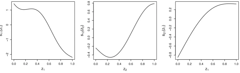
were considered, and sample sizes were set to 500, 1500 and 3000. For each combination of parameter settings, the number of simulated datasets was 250. Models were fitted with and without exclusion restriction (ER and non-ER, respectively). Specifically, in the latter casez2iwas not included in the selection equation.

[image:8.544.66.486.51.179.2]

Fig. 1. The test functions used in the simulation studies.

To make a fair comparison, the smooth components of the proposed method were represented usingP-splines with the same settings. Models were also fitted neglecting the sample selection issue: using the selected sample, simply fit Eq.(5)

via penalized least squares, again with the same number ofP-spline bases and penalty order. As this naive approach cannot correct sample selection bias, badly biased parameter estimates are clearly expected in the simulation results. However, reporting such results should be useful to highlight the negative effects that the neglect of non-random sample selection has on parameter estimates. Following a reviewer’s suggestion, we also employed a standard Heckman approach where non-linear effects were modeled using second-order polynomial terms.

3.1. Results

In this section, we only show a subset of results; these are representative of all empirical findings. Since the selection equation is not affected by sample selection bias, we focus on the estimation results for the outcome equation only.Table 1

reports the percentage relative bias and the root mean squared error (RMSE) for

θ

22

, ρ

and

σ

, when assuming that ER holds and approximately 50% of the total number of observations are available to fit the outcome equation. The approaches employed are naive, standard Heckman with second-order polynomial terms, and penalized Bayesian and ML estimation (naive, HeckP, W&K and M&R, respectively).Table 2shows the RMSE and 95% average coverage probability (ACP) for the four approaches when estimatings21

(

z1

)

under the same settings as described above.Tables 3and4report the bias and RMSE for

ˆ

θ

22

,

ρ

ˆ

and

σ

ˆ

, and RMSE and ACP for

ˆ

s21

(

z1

)

, respectively, for the non-ER case when approximately 75% of the total number of observations are selected for the outcome equation. This scenario should be reasonably close to the empirical illustration presented in Section4, where there is no ER and the 77% of observations are selected. The results for the non-ER case when approximately 50% of observations are selected are reported inAppendix D(Table 8).Table 5reports the results obtained under the ER scenario with 50% of selected observations when in the data generating process the simple non-linear function s21

(

z1

)

is swapped with functions11

(

z1

)

. In this case,

θ

11was set to

−

3.05. As inWiesenfarth and Kneib(2010), based on the estimates for 200 fixed covariate values, RMSE

(

ˆ

s

)

was calculated as





200

b=1



ˆ

s

(

z1b

)

−

s

(

z1b

)



2

. In terms of computing mean times, M&R showed lower computational cost than W&K. Specifically, mean times for M&R were between 0.02 and 0.17 min depending onnand

ρ

. Compared to M&R, W&K approximately took between 25 and 100 times longer to fit a sample selection model.

The main results can be summarized as follows.

•

Table 1shows that the neglect of non-random sample selection leads to seriously biased parameter estimates. When

ρ

is small, HeckP outperforms all other methods in terms of bias. However, as

ρ

increases (i.e., the sample selection issue becomes more pronounced), M&R and W&K outperform HeckP, with M&R being the best in terms of bias. For high

ρ

, M&R performs the best in terms of bias and precision. Asnincreases, the W&K, M&R and HeckP estimates show convergence to their true values. Similar conclusions are reached fors21

(

z1

)

(seeTable 2). The 95% ACPs for M&R are more accurate than those for W&K and HeckP. This suggests that a fully Bayesian approach, which accounts for smoothing parameter uncertainty, yields slightly conservative pointwise intervals. This finding supports the argument byMarra and Wood

(2012) (see Section2.3) and is in agreement with the results ofWiesenfarth and Kneib(2010). We did not report the ACPs for the biased naive fits because these were clearly below the nominal level.

•

In the non-ER case, when 50% of observations are selected (Table 8inAppendix D), all methods exhibit higher bias as compared to the ER case. In addition, similar trends as those inTables 1and2are detected, with W&K and M&R being the best and naive being the worst as

ρ

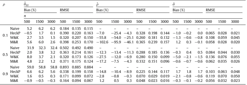
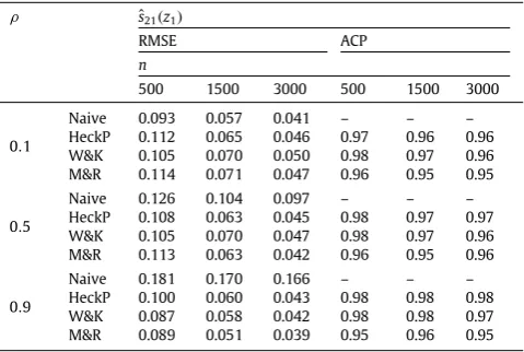
increases. When about three-fourth of the total number of observations are available for the outcome equation, the same patterns can again be observed but with lower bias and RMSE (seeTables 3and4). This finding complements the argument in the final paragraph of Section2.1by suggesting that the presence of ER is necessary to obtain good estimation results, unless the percentage of selected observations is high.

Table 1

Percentage biases and RMSEs forθˆ22,ρˆandσˆobtained from the ER experiments, when employing the naive, standard Heckman (with second-order polynomial terms), penalized Bayesian and ML estimation approaches (naive, HeckP, W&K and M&R). Number of simulated datasets and approximate percentage of selected observations are 250% and 50%. True values ofθ22andσare−1.5 and 1.ρandndenote the correlation between the errors of the selection and outcome equations, and the sample size. See Section3for further details.

ρ _θˆ₂₂ ρˆ σˆ

Bias (%) RMSE Bias (%) RMSE Bias (%) RMSE

n

500 1500 3000 500 1500 3000 500 1500 3000 500 1500 3000 500 1500 3000 500 1500 3000

0.1

Naive 5.2 6.2 6.2 0.184 0.135 0.115 – – – – – – – – – – – –

HeckP −0.5 1.7 0.1 0.390 0.220 0.163 −7.0 −25.4 −4.3 0.328 0.198 0.144 −1.0 −0.2 0.0 0.065 0.028 0.021 W&K 2.7 3.5 1.5 0.320 0.207 0.150 −55.8 −54.0 −25.1 0.260 0.181 0.132 −1.3 −0.6 −0.8 0.108 0.059 0.045 M&R 5.6 6.0 2.6 0.398 0.253 0.170 −102.6 −95.9 −46.1 0.365 0.239 0.157 1.2 0.3 −0.1 0.058 0.028 0.020

0.5

Naive 31.9 32.3 32.4 0.502 0.492 0.490 – – – – – – – – – – – –

HeckP 2.0 3.8 3.2 0.363 0.214 0.161 −12.3 −13.4 −11.3 0.288 0.185 0.136 −0.3 0.4 0.5 0.084 0.044 0.030 W&K 8.0 3.7 2.1 0.320 0.173 0.126 −27.5 −12.0 −6.9 0.280 0.150 0.099 −5.0 −2.1 −1.5 0.136 0.076 0.055 M&R 4.8 2.2 1.2 0.371 0.175 0.124 −17.2 −7.5 −4.3 0.332 0.151 0.096 −0.6 −0.7 −0.6 0.062 0.035 0.026

0.9

Naive 59.0 58.8 58.8 0.893 0.885 0.884 – – – – – – – – – – – –

[image:9.544.38.506.101.263.2] [image:9.544.152.391.324.486.2]

HeckP 6.6 6.2 5.6 0.338 0.199 0.158 −14.8 −10.4 −8.9 0.225 0.144 0.117 1.7 1.8 1.7 0.103 0.063 0.048 W&K 1.6 0.5 0.3 0.171 0.099 0.072 −2.8 −0.8 −0.3 0.070 0.029 0.019 −2.1 −0.8 −0.6 0.119 0.070 0.050 M&R −0.9 −0.5 −0.3 0.164 0.094 0.067 1.2 0.5 0.3 0.048 0.023 0.016 −0.3 −0.1 −0.2 0.056 0.032 0.023

Table 2

RMSEs and 95% average coverage probabilities forˆs21(z1)obtained from the ER experiments, when employing naive, HeckP, W&K and M&R. Number of simulated datasets and approximate percentage of selected observations are 250% and 50%. See the caption ofTable 1for further details.

ρ ˆs21(z1)

RMSE ACP

n

500 1500 3000 500 1500 3000

0.1

Naive 0.121 0.075 0.059 – – – HeckP 0.143 0.079 0.056 0.97 0.97 0.96 W&K 0.137 0.085 0.066 0.98 0.97 0.97 M&R 0.164 0.099 0.069 0.96 0.96 0.95

0.5

Naive 0.200 0.185 0.178 – – – HeckP 0.135 0.076 0.055 0.97 0.97 0.97 W&K 0.134 0.078 0.058 0.97 0.97 0.97 M&R 0.146 0.080 0.056 0.96 0.96 0.96

0.9

Naive 0.314 0.311 0.309 – – – HeckP 0.124 0.073 0.056 0.98 0.97 0.98 W&K 0.099 0.065 0.049 0.98 0.98 0.97 M&R 0.101 0.062 0.043 0.96 0.96 0.95

previous case, this scenario better highlights the advantage of penalized regression splines over polynomial models. Overall, results show that HeckP does not model adequately regressor effects. Specifically, for any value of

ρ

andn, the HeckP RMSE of

ˆ

s11

(

z1

)

is consistently higher than that of M&R. In addition, the residual confounding induced by the mismodeled non-linear effects seems to have negative consequences on the estimation of the parametric effects, where HeckP underperforms in terms of accuracy and precision.

•

We also carried out additional simulation experiments where the model errors are generated according to a bivariate Student-tdistribution with 3 degrees of freedom; seeTables 9and10inAppendix D. As expected, results are worse than those presented in this section. However, the use of ER helps to obtain better estimates although still not as good as those produced when the assumption(3)is met. Even worse results (available upon request) are found when using asymmetric or bimodal bivariate model error distributions, case in which the presence of ER cannot really help. The reason for this result is that the likelihood of the model is wrongly specified (i.e., we assume normality but the model errors are generated from a Student-tdistribution) and ML approaches are known to be sensitive to such issues.

Table 3

Percentage biases and RMSEs forθˆ22,ρˆandσˆobtained from the non-ER experiments, when employing the naive, standard Heckman (with second-order polynomial terms), penalized Bayesian and ML estimation approaches (naive, HeckP, W&K and M&R). Number of simulated datasets and approximate percentage of selected observations are 250% and 75%. See the caption ofTable 1for further details.

ρ _θˆ

22 ρˆ σˆ

Bias (%) RMSE Bias (%) RMSE Bias (%) RMSE

n

500 1500 3000 500 1500 3000 500 1500 3000 500 1500 3000 500 1500 3000 500 1500 3000

0.1

Naive 3.1 3.3 3.4 0.136 0.088 0.072 – – – – – – – – – – – –

HeckP −0.1 0.4 −0.6 0.297 0.173 0.122 −24.8 −26.0 3.0 0.431 0.253 0.188 −1.6 −0.5 −0.2 0.065 0.029 0.019 W&K 1.8 1.9 0.6 0.200 0.145 0.099 −60.8 −59.8 −25.7 0.278 0.218 0.150 −3.9 −1.4 −1.2 0.099 0.051 0.040 M&R 2.4 2.2 0.7 0.253 0.159 0.105 −83.4 −70.4 −29.3 0.378 0.252 0.168 1.1 0.5 0.1 0.047 0.023 0.016

0.5

Naive 17.1 17.5 17.5 0.285 0.271 0.267 – – – – – – – – – – – –

HeckP 1.6 1.6 0.7 0.290 0.171 0.118 −28.0 −20.6 −15.2 0.408 0.253 0.187 −0.8 0.1 0.2 0.080 0.038 0.029 W&K 6.9 3.0 1.8 0.233 0.138 0.090 −47.1 −24.0 −15.5 0.365 0.210 0.139 −7.0 −3.2 −1.8 0.130 0.071 0.051 M&R 5.1 1.3 0.8 0.261 0.126 0.083 −36.7 −14.4 −11.1 0.415 0.190 0.119 −0.4 −0.4 −0.5 0.050 0.028 0.021

0.9

Naive 31.2 31.6 31.6 0.481 0.478 0.477 – – – – – – – – – – – –

[image:10.544.43.508.92.255.2] [image:10.544.155.395.312.473.2]

HeckP 2.3 3.0 1.9 0.272 0.159 0.117 −25.4 −19.6 −15.7 0.367 0.249 0.199 0.8 1.5 1.2 0.096 0.056 0.045 W&K 2.3 0.5 0.4 0.159 0.078 0.055 −14.0 −8.1 −7.8 0.205 0.090 0.080 −4.8 −1.5 −1.7 0.130 0.060 0.045 M&R 0.4 −0.1 0.1 0.147 0.073 0.053 −7.6 −6.3 −6.6 0.174 0.068 0.065 −0.8 −0.4 −0.5 0.048 0.025 0.019

Table 4

RMSEs and 95% average coverage probabilities forˆs21(z1)obtained from the non-ER experiments, when employing naive, HeckP, W&K and M&R. Number of simulated datasets and approximate percentage of selected observations are 250% and 75%. See the caption ofTable 1for further details.

ρ ˆs21(z1)

RMSE ACP

n

500 1500 3000 500 1500 3000

0.1

Naive 0.093 0.057 0.041 – – – HeckP 0.112 0.065 0.046 0.97 0.96 0.96 W&K 0.105 0.070 0.050 0.98 0.97 0.96 M&R 0.114 0.071 0.047 0.96 0.95 0.95

0.5

Naive 0.126 0.104 0.097 – – – HeckP 0.108 0.063 0.045 0.98 0.97 0.97 W&K 0.105 0.070 0.047 0.98 0.97 0.96 M&R 0.113 0.063 0.042 0.96 0.95 0.96

0.9

[image:10.544.42.508.526.635.2]

Naive 0.181 0.170 0.166 – – – HeckP 0.100 0.060 0.043 0.98 0.98 0.98 W&K 0.087 0.058 0.042 0.98 0.98 0.97 M&R 0.089 0.051 0.039 0.95 0.96 0.95

Table 5

Percentage biases and RMSEs forθˆ22,ρ,ˆ σˆ andˆs11(z1)obtained from the ER experiments, when employing the standard Heckman (with second-order polynomial terms) and ML estimation approaches (HeckP and M&R). Number of simulated datasets and approximate percentage of selected observations are 250 and 50%. See Section3for further details.

ˆ

θ22 ρˆ σˆ ˆs11(z1)

Bias (%) RMSE Bias (%) RMSE Bias (%) RMSE RMSE

n

500 3000 500 3000 500 3000 500 3000 500 3000 500 3000 500 3000

0.1 HeckP 6.0 7.1 0.644 0.272 −87.7 −87.4 0.425 0.194 −2.5 −1.5 0.071 0.030 1.564 1.564 M&R −0.1 −0.3 0.662 0.256 −30.3 −5.0 0.359 0.168 −0.9 0.0 0.064 0.021 1.526 1.528

0.5 HeckP 8.6 7.8 0.584 0.257 258.7 296.4 0.444 0.335 −1.4 −0.8 0.069 0.029 1.569 1.565 M&R −0.5 −0.6 0.573 0.241 −21.7 −5.3 0.335 0.147 −0.6 0.0 0.081 0.030 1.511 1.523

0.9 HeckP 9.3 8.0 0.561 0.233 607.7 694.7 0.664 0.705 −0.3 0.0 0.091 0.034 1.572 1.566 M&R 2.4 −1.5 0.510 0.211 −18.6 −2.9 0.282 0.077 −0.2 −0.3 0.103 0.044 1.501 1.519

4. Empirical illustration

[image:11.544.106.438.71.257.2]

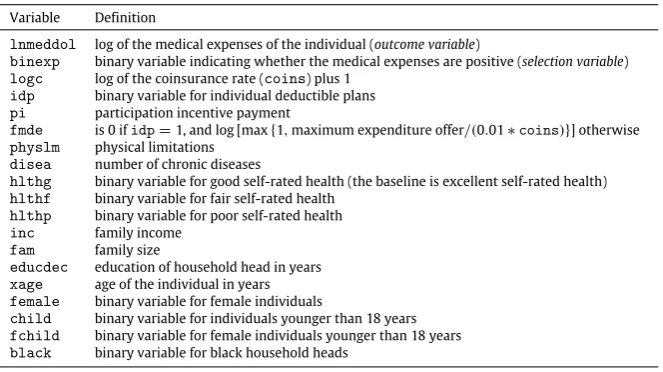
Table 6

Description of the outcome and selection variables, and of the regressors.

Variable Definition

lnmeddol log of the medical expenses of the individual (outcome variable)

binexp binary variable indicating whether the medical expenses are positive (selection variable) logc log of the coinsurance rate (coins) plus 1

idp binary variable for individual deductible plans pi participation incentive payment

fmde is 0 ifidp=1, and log [max{1,maximum expenditure offer/(0.01∗coins)}] otherwise physlm physical limitations

disea number of chronic diseases

hlthg binary variable for good self-rated health (the baseline is excellent self-rated health) hlthf binary variable for fair self-rated health

hlthp binary variable for poor self-rated health inc family income

fam family size

educdec education of household head in years xage age of the individual in years female binary variable for female individuals

child binary variable for individuals younger than 18 years fchild binary variable for female individuals younger than 18 years black binary variable for black household heads

utilization and outcome conducted in the United States between 1974 and 1982 (Newhouse, 1999). As explained in the introductory section, the aim was to quantify the relationship between various covariates and annual health expenditures in the population as a whole.

In this context, non-random sample selection arises because the sample consisting of individuals who used health care services differ in important characteristics from the sample of individuals who did not use them. Because some characteristics cannot be observed, traditional regression modeling is likely to deliver biased estimates. We, therefore, need to correct parameter estimates for sample selection bias. We use the same subsample as inCameron and Trivedi(2005,

p. 553), and model annual health expenditures. The sample size and number of selected observations are 5574 and 4281. The variables are defined inTable 6. Additional information can be found inCameron and Trivedi(2005,Table 20.4) and

Newhouse(1999).

FollowingCameron and Trivedi(2005) the outcome and the selection equations include the same set of regressors. In M&R and W&K, the two equations include

logc

,

idp

,

fmde

,

physlm

,

disea

,

hlthg

,

hlthf

,

hlthp

,

female

,

child

,

fchild

and

black

as parametric components, and smooth functions of

pi

,

inc

,

fam

,

educdec

and

xage

, represented usingP-spline bases with 20 inner knots and penalty matrices based on second order differences. For naive, the same model specification is adopted but clearly a selection equation is not present. As for standard Heckman, we model the effects of

pi

,

inc

,

fam

,

educdec

and

xage

using second-order polynomials. For W&K, the number of iterations for burn-in, of samples used for estimation, and degree of thinning were the same as those employed in the simulation study.

The use of smooth functions for

xage

,

educdec

and

inc

is suggested by the fact that these covariates embody productivity and life-cycle effects that are likely to influence health expenditures non-linearly.Dismuke and Egede(2011) andSullivan et al.(2007) consider parametric specifications where non-linear effects are modeled by categorizing these variables into groups based on intervals. However, categorizing a continuous variable has several disadvantages since, for example, it introduces problems of defining cut-points and assumes a priori that the relationship between response and covariate is flat within intervals (e.g.,Marra and Radice, 2010). As for

fam

and

pi

, we do not have a priori knowledge of their effects and imposing linear or quadratic relationships may prevent us from revealing interesting non-linear relationships. Smooth functions of other covariates such as

idp

and

disea

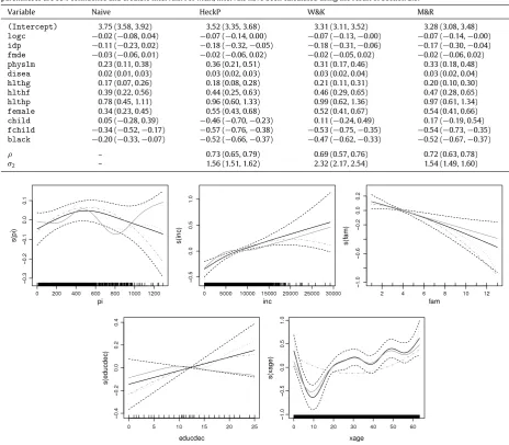
are not considered as their number of unique covariate values is too small.

Table 7andFig. 2report the parametric and smooth function estimates for the outcome equation (which is the one of interest) when applying the four approaches on the RAND RHIE dataset. Computational times for M&R and W&K were 1.03 and 18.26 min, respectively.

The parametric effects obtained using HeckP, M&R and W&K are very similar (except for the effect of

child

) and differ from those of naive. Specifically, the M&R and W&K results suggest that socioeconomic factors (

black

,

female

,

child

, and

fchild

) as well as health status variables (

physlm

,

disea

,

hlthg

,

hlthf

,

hlthp

) have a stronger effect on annual health expenses as compared to the naive results. The health insurance variables (

logc

,

idp

) seem not to determine the annual medical expenses when using naive. The estimated smooths for the socioeconomic variables (

inc

,

fam

,

educdec

[image:12.544.40.505.86.492.2]

Table 7

Parametric estimates of the annual medical expense equation obtained by applying the naive, standard Heckman (with second-order polynomial terms), penalized Bayesian and ML estimation approaches (naive, HeckP, W&K and M&R, respectively) on the RAND RHIE dataset described in Section4. Within parentheses are 95% confidence and credible intervals. For M&R, intervals have been calculated using the result of Section2.3.

Variable Naive HeckP W&K M&R

(Intercept) 3.75 (3.58, 3.92) 3.52 (3.35, 3.68) 3.31 (3.11, 3.52) 3.28 (3.08, 3.48) logc −0.02 (−0.08, 0.04) −0.07 (−0.14, 0.00) −0.07 (−0.13,−0.00) −0.07 (−0.14,−0.00) idp −0.11 (−0.23, 0.02) −0.18 (−0.32,−0.05) −0.18 (−0.31,−0.06) −0.17 (−0.30,−0.04) fmde −0.03 (−0.06, 0.01) −0.02 (−0.06, 0.02) −0.02 (−0.05, 0.02) −0.02 (−0.06, 0.02) physlm 0.23 (0.11, 0.38) 0.36 (0.21, 0.51) 0.31 (0.17, 0.46) 0.33 (0.18, 0.48) disea 0.02 (0.01, 0.03) 0.03 (0.02, 0.03) 0.03 (0.02, 0.04) 0.03 (0.02, 0.04) hlthg 0.17 (0.07, 0.26) 0.18 (0.08, 0.28) 0.21 (0.11, 0.31) 0.20 (0.10, 0.30) hlthf 0.39 (0.22, 0.56) 0.44 (0.25, 0.63) 0.46 (0.29, 0.65) 0.47 (0.28, 0.65) hlthp 0.78 (0.45, 1.11) 0.96 (0.60, 1.33) 0.99 (0.62, 1.36) 0.97 (0.61, 1.34) female 0.34 (0.23, 0.45) 0.55 (0.43, 0.68) 0.52 (0.41, 0.67) 0.54 (0.41, 0.66) child 0.05 (−0.28, 0.39) −0.46 (−0.70,−0.23) 0.11 (−0.24, 0.49) 0.17 (−0.19, 0.54) fchild −0.34 (−0.52,−0.17) −0.57 (−0.76,−0.38) −0.53 (−0.75,−0.35) −0.54 (−0.73,−0.35) black −0.20 (−0.33,−0.07) −0.52 (−0.66,−0.37) −0.47 (−0.62,−0.33) −0.52 (−0.67,−0.37)

ρ – 0.73 (0.65, 0.79) 0.69 (0.57, 0.76) 0.72 (0.63, 0.78)

σ2 – 1.56 (1.51, 1.62) 2.32 (2.17, 2.54) 1.54 (1.49, 1.60)

Fig. 2. Smooth function estimates obtained by applying naive (gray lines), HeckP (gray dot-dashed lines), W&K (gray dotted lines) and M&R (black lines) on the RAND RHIE dataset described in Section4. The black dashed lines represent 95% pointwise confidence intervals calculated from the M&R estimates. The ‘rug plot’, at the bottom of each graph, shows the covariate values. To avoid clutter, credible intervals for W&K have not been reported. Due to the identifiability constraints, the estimated curves are centered around zero.

with that found in the simulated non-ER scenario with percentage of selected observations equal to 75%. Overall, the M&R and W&K estimates are coherent with the predictions of economic theory. For example, the results of age, education and income are consistent with the interpretation that health expenditure increases as people become older, have more years of schooling, and are wealthier. Also, individual health expenditure decreases as family size increases.

spline is approximately equivalent to a pure regression spline with degrees of freedom close to that of the penalized fit (e.g.,

Wood, 2006, pp. 210–212). This topic is beyond the scope of this paper and will be addressed in future research.

5. Conclusions

We introduced an algorithm to estimate a regression spline sample selection model for Gaussian data. The proposal is based on the penalized likelihood estimation framework. The construction of confidence intervals has also been illustrated, and the problem of identification has been discussed. The method has been tested and compared to a Bayesian counterpart and the classic Heckman sample selection model. Finally, the proposed approach and its competitors have been illustrated on data from the RAND Health Insurance Experiment on annual health expenditures. The

R

package

SemiParSampleSel

(Marra and Radice, 2012) implements the ideas discussed in this article.

The results of our simulation study highlighted the detrimental effects that the neglect of non-random sample selection has on parameter estimation. They also suggested that the two Bayesian and ML regression spline approaches considered in this article are effective and generally outperform standard Heckman with polynomials. The Bayesian and ML methods were found to perform similarly, with the former being more computationally expensive than the latter. We also found that ER is generally required to obtain good estimation results.

Because ML estimators are sensitive to model error misspecification, methods allowing for different bivariate distributions of the errors can be developed. For example,Marchenko and Genton(2012) introduced a sample selection model where the errors are assumed to follow a bivariate Student-t distribution. However, in their implementation the structure of the linear predictor is parametrically pre-specified. The proposed approach could be extended by adopting either a copula (e.g.,Nelsen, 2006) or a nonparametric distribution function estimation framework. Future research will be conducted toward these directions.

Acknowledgments

Giampiero Marra was supported by the Engineering and Physical Sciences Research Council (grant EP/J006742/1). We are indebted to the Editor, Associate Editor and two reviewers for the detailed comments, which helped us improve the manuscript and clarify the main messages.

Appendix A. Analytical expressions forgandH

The expressions for the gradient vector and Hessian matrix that are referred to in Section2.2are given below. Let us defineX_vi

=



uT

vi

,

B T

vi



for

v

=

1

,

2

, σ

2

=

exp

(σ

2∗

), ρ

=

tanh

(ρ

∗

_),

_e

2i

=

y2i

−

η

2i

,

a

=



1

−

ρ

2

,

_A

i

=

(η

1i

+

ρ

σ2e2i

)/

a

,

l1i

=

φ(

−

η

1i

)/

Φ

(

−

η

1i

),

l2i

=

φ(

Ai

)/

Φ

(

Ai

),

ec

=

exp

(

2

ρ

∗

_),

_PA

i

= −



Φ

(

Ai

)φ(

Ai

)

Ai

+

φ(

Ai

)

2



/

Φ

(

Ai

)

2

,

PEi

=

−



−

Φ

(

−

η

_1i

)φ(

−

η

_1i

)η

_1i

+

φ(

−

η

_1i

)

2



/

Φ

(

−

η

_1i

)

2

,

R

= {

4

ρ

ec

(ρ

−

1

)

}

/(

ec

+

1

),

Mi

=

(

2ece2i

)/

{

(

ec

+

1

)σ

2a

}

andC

=

−

1

+

ρ

+



ρ

2

_(ρ

₋

₁

₎



/

a2_{. The remaining quantities are defined in Section2.} The elements of the score vector are

g1

=

n



i=1



−

(

1

−

y1i

)

l1i

+

y1il2i

a



X1i

,

g2

=

n



i=1 y1i



e2i

σ

2 2

−

l2i

ρ

σ

2a



X2i

,

g3

=

n



i=1 y1i



−

1

+



e2i

σ

2



2

−

l2i

ρ

e2i

σ

2a



,

g4

=

n



i=1 y1i



l2i



Mi

(

1

−

ρ)

−

AiR 2a2



.

The elements of the Hessian are

H11

=

n



i=1



(

1

−

y1i

)

PEi

+

y1iPAi

a2



XT 1iX1i

,

H12

=

n



i=1



−

y1iPAi

ρ

σ

2a2



XT 1iX2i

,

H13

=

n



i=1



−

y1iPAi

ρ

e2i

σ

2a2

