Implementation of a Bayesian linear regression framework for nuclear prognostics

Nuclear Prognostics

Omer Panni1, Graeme West2, Victoria Catterson3, Stephen McArthur4, Dongfeng Shi5and Ieuan Mogridge6 1,2,3,4_{University of Strathclyde, Glasgow, G1 1XW, United Kingdom}

[email protected] [email protected] [email protected] [email protected]

5_{Rolls-Royce Control and Data Services Ltd, Derby, DE24 8BJ, United Kingdom}

[email protected]

6_{EDF Energy, Gloucester, GL4 3RS, United Kingdom}

[email protected]

ABSTRACT

Steam turbines are an important asset of nuclear power plants (NPPs), and are required to operate reliably and ef-ficiently. Unplanned outages have a significant impact on the ability of the plant to generate electricity. Therefore, predictive and proactive maintenance which can avoid un-planned outages has the potential to reduce operating costs while increasing the reliability and availability of the plant.

A case study from the data of an operational steam tur-bine of a NPP in the UK was used for the implementation of a Bayesian Linear Regression (BLR) framework. An appropriate model for the deterioration under study is se-lected. The BLR framework was applied as a prognostic technique in order to calculate the remaining useful life (RUL). Results show that the accuracy of the technique varies due to the nature of the data that is utilised to esti-mate the model parameters.

1. INTRODUCTION

Steam turbines are expensive and an important part of a nu-clear power plant. The consequences of technical failure could compromise the safe and economic operation of the plant. An effective condition monitoring system ensures that the plant is operating in acceptable condition by providing accurate in-formation about the current health of the plant. This work Omer Panni et al. This is an open-access article distributed under the terms of the Creative Commons Attribution 3.0 United States License, which permits unrestricted use, distribution, and reproduction in any medium, provided the original author and source are credited.

investigates the use of prognostic techniques to predict future health of steam turbine assets.

The main aim of prognostics is to estimate the remaining use-ful life of the asset and provide decision support for mainte-nance when the asset is in service. Prognostics have been successfully applied to a wide range of maintenance and re-liability applications in the industries of aerospace (Zaidan et al., 2013; Qiancheng et al., 2011; Saha et al., 2009), power networks (Catterson et al., 2016; Rudd et al., 2011), defence (Hess & Fila, 2002), consumer electronics (Gu et al., 2009; Zheng et al., 2014) and nuclear generation (Di Maio et al., 2011; Coble et al., 2010). The main advantages of prognos-tics are reduction in unplanned outages, increased reliabil-ity and availabilreliabil-ity, and reduced life-cycle costs (Sun, Zeng, Kang, & Pecht, 2012).

ex-pansion between the turbine casing and the supports. When investigating the fault, the broad engineering judgement was that this fault manifested itself as a linear relationship and hence the choice of a linear model. Subsequent analysis has shown this assumption to be incorrect over the full span of the degradation and an important outcome of this work is to rec-ommend a more representative model of degradation be cho-sen. However, this case study is still useful for explaining the development and deployment of prognostic techniques within a nuclear environment.

2. APPLICATIONREQUIREMENTS

This paper focuses on a particular case study fault within the High Pressure (HP) steam turbine of a nuclear power plant in the UK. Figure 1 shows the general representation of the arrangement for handling thermal expansion in a steam tur-bine. The outer casing palms of the HP cylinder lean on the transversal keys attached to the bearing pedestals. The transversal keys guide the lateral thermal expansion of the casing. The bottom of the bearing pedestals is attached to the longitudinal keys allowing the bearing pedestal to slide on the foundation frame when the metal temperature of the turbine varies during the start-up (runup) and stop (rundown) operating conditions (Leyzerovich, 2008).

Figure 1. General Steam Turbine Arrangement (Leyzerovich, 2008)

The entire weight of the steam turbine rests on the bearing pedestals, as a result of which substantial frictional forces are produced which hinder the axial movement of the bear-ing pedestal along the foundation frame. As a result, this can manifest in an increased displacement of the HP shaft, and in an increased level of vibration within the bearings. The fault is slow and progressive, in that without intervention the level of displacement increases over time which can result in distortion of the casing, increased vibration, damage to the turbine bearings and couplings etc. However, if the turbine is taken offline or stopped and the casing cools sufficiently, the displacement may reduce as well.

This fault was observed within one turbine, fully analysed by the engineers, and corrective action taken by changing the interface between the pedestal and foundation from injected grease (which was inserted at first as a remedial solution to

re-duce friction) to a self-lubricating graphite-impregnated ma-terial. However, there is a desire to develop an automated system that can detect the presence of this specific fault, and predict the time remaining until the displacement reaches a level requiring intervention. The intervention threshold is de-rived from ISO 7919-2:2009 (BSI, 2009), an industry stan-dard which defines a warning threshold at 82.5um of dis-placement. Therefore, the aim of the prognostic system is to predict the RUL until displacement reaches82.5um. Since there is only a single case study instance of this fault captured, the approach to developing the prognostic system must utilise engineering judgement in combination with the case study data. Expertise from the plant engineer suggested that casing expansion was expected to increase linearly over time without intervention. This broadly matched the pattern seen within the case study data (see Section 3.1).

Another application requirement is that RUL prediction er-rors should tend to be early rather than late. If the prediction is late (ie failure occurs earlier than predicted), maintenance may not be scheduled in time to prevent the failure. On the other hand, if the prediction is early (ie failure occurs later than predicted), maintenance may be scheduled earlier than needed, leading to more interventions over time with associ-ated higher costs and downtime. While the prediction should be as accurate as possible, the consequences of a late predic-tion are more significant than those of an early predicpredic-tion, and therefore early predictions are preferred.

BLR was selected as a technique which can meet these cri-teria. The main advantage of using BLR is that it estimates RUL in the form of a probability distribution to avoid the risk of early failure. BLR updates the degradation model using the degradation history and current degradation data, as a re-sult of which uncertainty in degradation model parameters is reduced.

3. DATAANALYSIS

Data was captured from the turbine from various operational states, including online, run down, and run up conditions. For a typical day, data is usually recorded in a single file. However, during fault conditions, the data logging system can record multiple files within one day by changing the data log-ging frequency. The dataset studied here consisted of 6685 files, containing measurement parameters such as bearing ve-locity, shaft displacement, and generated power. The data was then segregated based on the operational states.

summarised. In other words, each parameter in each file was represented by one value. A window of the online profile of mean power is shown in Figure 2.

Figure 2. Mean Online Power

Figure 2 shows the variation in mean power across a period of approximately 15 months. The power fluctuates according to the operational state of the turbine. Most of the time it oper-ates at full power, 660 MW approx. During refuelling outages the power is lowered to 70% of full power then dropped to 30%while fuel assemblies are exchanged. The data relating to refuelling events was removed, as changes in power were clearly seen to influence vibration data, and therefore made it difficult to identify any pattern visually by considering this full set of data across all power levels. From here on, this dataset is referred as the Full Power dataset.

3.1. High Pressure (HP) Turbine Displacement

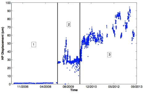
Through visual analysis of the Full Power dataset, three pat-terns in HP displacement that are labelled with region num-bers in Figure 3 were observed. In region 1, there is very low displacement and after this region a step change is observed which is due to a change in operational settings. In region 2, displacement tends to remain relatively steady with fluctua-tions towards the start. In region 3, a ramp up in displacement can be observed. This behaviour has been investigated by the diagnostic engineer, and is attributed to thermal expansion of the casing of the steam turbine.

The gaps in the HP Displacement data are due to the removal of the outages/stoppage durations, online data captured below full power, and other vibration data captured during the state of run up.

3.2. Change Point Analysis

Change point analysis is used to find the location of points within a data sequence where there are significant changes. The location of the change point is the maximum or mini-mum point in a vector of the sum of differences between each

Figure 3. HP Displacement

data point and the mean of all data points. Additional change points can be determined within a region by repeating the pro-cess (Killick & Eckley, 2014).

Change point analysis was applied to the HP displacement to identify points of deviation. This technique identifies change points in iterations. For HP displacement, two iterations were performed based on the observation of the online full power HP displacement data. In the first iteration, the cumulative sum of the difference of the online full power HP displace-ment data from its mean was calculated, which resulted in the change point 1 as shown in Figure 4. This change point is the lowest cumulative sum of the difference between the data points and their mean.

Figure 4. Cumulative Sum Of HP Displacement

Figure 5. HP Ramp Case Study

4. BAYESIANLINEARREGRESSION

Based on the broad engineering judgement, the fault mani-fested itself as a linear relationship and therefore, first order polynomial is selected as a degradation model (see Section 2). A first order polynomial function is a straight line which has two parameters: the slope and the y-intercept which can be expressed asw =

w0

w1

, wherew0 is the intercept and

w1 is the slope. Bayesian Linear Regression (BLR) starts

with no knowledge aboutw, therefore, without any knowl-edge of a straight line representing the degradation trend. If predictions of RUL are made at this stage, the output will be random. This belief aboutwbefore any data is observed can be represented as a probability distribution. This probabil-ity distribution is known as a prior or prior probabilprobabil-ity distri-bution. As data is observed (i.e. measurements of HP Dis-placement are made), the likelihood of the data can be calcu-lated as a conditional probability of the data given the straight line parameters. BLR uses observed data to update the prior probability ofw to form a posterior distribution ofw. The posterior distribution narrows down the set of likely straight lines which best fit the degradation trend. After enough data has been observed, the uncertainty inw(or the slope and the y-intercept) has been reduced so that relatively few straight lines are candidates for the “true” degradation trend. At this point, predictions of the RUL cover a fairly narrow range of values, since all candidate straight lines reach the threshold around the same time.

Bayesian Linear Regression (BLR) uses Bayes theorem to convert the prior probability of the model parameters (the slope and the y-intercept) into posterior probability by incor-porating the evidence provided by the data in the form of the likelihood function. The Bayes theorem in generalised form (Bishop, 2006) is expressed as:

p(w|D) =p(D|w)p(w)

p(D) (1)

wherep(w|D)is the posterior probability distribution,p(D|w)

is the likelihood function,p(w)is the prior probability distri-bution andp(D)is the probability of the data. Alternatively according to (Gelman et al., 2004), given the above definition of the likelihood function, Bayes theorem can be expressed as:

posterior∝likelihood×prior (2)

4.1. Model Setup

According to (Murphy, 2012), before the application of BLR, degradation is modelled as:

y=φ(x)Tw+ (3) wherey is the degradation signal (HP displacement in our case), is random error, wis vector of weights (the slope and the y-intercept) andφ(x)T is first order polynomial ba-sis withxdenoting time. The first order polynomial basis function in reduced form can be represented as: φ(x)T_{w =}

1 x1

w0

w1

.

4.2. Bayesian Linear Regression Framework

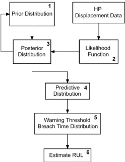
As shown in Figure 6, there are six parts in the Bayesian Lin-ear Regression (BLR) framework. For the first three parts of the BLR Framework, Bayes theorem is applied to update the prior probability distribution of the model parameters to form a posterior distribution with the likelihood of the ob-servation data. Once the model parameters w(or the slope and the y-intercept) are updated, they are used to get the pre-dicted signal over the desired time as shown by “predictive distribution” in Figure 6. In the final step of Figure 6, the warning threshold breach time distribution is obtained to es-timate warning threshold breach timeT, in order to calculate the remaining useful life.

The following subsections describe each step in more detail.

4.2.1. Prior Distribution

The weights are modelled as a multivariate normal distribu-tion to capture the variable dependency. (In the case of a lin-ear model there are two dimensions to the distribution, one each forw0andw1). Therefore, the prior distribution can be

specified as:

p(w) =N(w|m0, S0) (4)

For simplicity, the prior is modelled as a zero mean Gaussian distribution so thatm0 = 0andS0 = α−1I withα → 0.

Therefore, when no data is observed the posterior distribu-tion is the same as the prior distribudistribu-tion. Also, when data points arrive sequentially, the posterior distribution acts as a prior distribution for the subsequent data point. In zero mean Gaussian distribution form, the prior can be expressed as:

p(w|α) =N(w|0, α−1I) (5) The value of the parameter αselected is 2. Several initial values of the parameterαwere tested and it made little to no difference to the output as its effect tends to diminish very quickly.

4.2.2. Likelihood

The likelihood is the conditional probability of the observed dataxand the model parameters(w, β), and is given by:

p(y|x, w, β) =N(φ(x)Tw, β−1) (6) whereβ is called the noise precision parameter. Similar test-ing was performed for parameterβas forα, and the value for parameterβselected is 25.

4.2.3. Posterior Distribution

According to Equation (5), the posterior distribution is pro-portional to the product of the likelihood function and the prior distribution. Mathematically it can be expressed as:

p(w|x, y, α, β)∝p(y|x, w, β)p(w|α) (7) Due to the fact that the prior has been chosen to be a conjugate normal distribution, the posterior distribution is also normal and therefore can be expressed as:

p(w|x, y, α, β) =N(y|m(x), s2(x)) (8) wheres2_(x)−1_=S−1

0 +βx

T_{xandm(x) =s}2_(x)(S−1 0 m0+

βxT_{y). Since the prior has been modelled as a zero mean} Gaussian distribution, therefore,s2_(x)−1_=αI+βxT_xand m(x) =βs2_(x)xT_{y. As mentioned earlier, due to the choice} of prior, the posterior distribution acts as a prior distribution for the subsequent data point when data points arrive sequen-tially. The resulting posterior is also used to compute the

pre-dictive distribution.

4.2.4. Predictive Distribution

The posterior distribution results in update of the model pa-rametersw, which can be used to make predictions ofyat a given future point in time. Therefore, the predictive distribu-tion is evaluated using the following equadistribu-tion:

p(ynew|y, α, β) =

Z

p(y|x, w, β)p(w|x, y, α, β) (9)

This predictive distribution represents the predicted degrada-tion signalynewprobabilistically. The predictive distribution can also be expressed as:

p(ynew|x, y, α, β) =N(y|m(x)Tx, σ2N(x)) (10) whereσ2_N(x) = _β1 +xTs(x)x. It should be noted that the predicted values ofynewcorrespond to a Normal distribution rather than one single value. This is fundamentally because of the uncertainty in the model parametersw: there is uncer-tainty in the slope of the linear trendw1and in the intercept

w0. The distribution ofynewvalues is the result of combining predictions from all linear trends within the envelope of pos-sible parameters. This is one of the key benefits of the BLR framework, i.e. that it can explicitly track the uncertainty in the linear model itself.

4.2.5. Warning Threshold Breach Time Distribution

As discussed in Section 2, the application places two require-ments on the handling of the displacement threshold. First, the threshold itself is set to82.5um, which is defined in ISO 7919-2:2009 as a warning limit. That means that when dis-placement breaches this threshold,yT hresh, there is still time for the plant operator to intervene before more serious limits are reached.

Within the case study data, the point of threshold breach has been defined as the mean time of the first 20 data points to breachyT hresh. This was chosen because a single data point may breach the threshold due to transient behaviour, but 20 data points represents a more consistent trend. This mean time of threshold breach is considered the true end-of-life point that the prognostic system should predict.

Secondly, early predictions are preferred over late predictions. In order to reduce the chance of late predictions, a Warning Threshold Breach Time Distribution is obtained by noting all possible predicted threshold breach timest. The predicted threshold breach timetis the predicted end-of-life point when the mean of the predictive distributionynew reaches or ex-ceeds the thresholdyT hresh. Together, all values oftgive a distribution of predictions.

breach times t was chosen as T, there would be an equal chance of early and late predictions. By selecting an earlier point, late predictions should be less likely.

4.2.6. Remaining Useful Life

RUL is the remaining time before the degradation signal crosses the threshold and can be calculated as:

RU L=T−xt (11)

whereT is the warning threshold breach time and xtis the current time or the time of the prognosis.

5. RESULTS& DISCUSSION

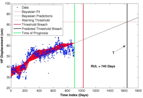
The HP displacement case study was used to assess the per-formance of the developed algorithm. Figure 7 and Figure 8 show RUL estimates when 300 and 400 data points of the HP displacement case study are used respectively. It can be seen that the implemented algorithm estimates the future health of the steam turbine using the case study data (blue dots).

Figure 7. RUL Predictions: 300 Data Points

Figure 8. RUL Predictions: 400 Data Points

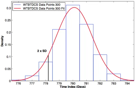
The distributions of warning threshold breach timestfor the batch of 300 and 400 data points are shown in Figure 9 and Figure 10.

Figure 9. Warning Threshold Breach Time Predictions: 300 Data Points

Figure 10. Warning Threshold Breach Time Predictions: 400 Data Points

As described in Section 4.2.5, a value of two standard devi-ations from the mean was chosen as the warning threshold breach timeT.

The comparison of true RUL and predicted RUL is given in Table 1. The results show that when 300, 350, 400 and 450 data points of the HP displacement case study are fed into the BLR framework, early prediction of warning threshold breach is observed which is due to increase in HP displace-ment data just before the time of prognosis (represented as solid green lines in Figure 7 and Figure 8). It should also be noted that due to the slow and progressive nature of the fault, large values of RUL predictions are observed.

con-Table 1. Early Prediction: Comparison of True RUL and Pre-dicted RUL

Set Of Data Points

True RUL (Days)

Predicted RUL (Days)

Prediction (Early or

Late)

300 726 478 248 Early

350 676 396 280 Early

400 626 414 212 Early

450 576 502 74 Early

sider further.

First, the errors in Table 1 are generally large. If the error is over 200 days, there is a significant amount of remaining life that may be lost through early scheduling of maintenance. While early predictions are preferred, overall accuracy is also important.

Secondly, and more critically, the performance of the algo-rithm tends to vary with different amounts of input data. For instance, when batches of 500 and 900 datapoints are used, the predictions are late as shown in Figures 11 and 12.

Figure 11. Late RUL Predictions: 500 Data Points The comparison of true RUL and predicted RUL is given in Table 2. The results show that the technique does generate late predictions. When it may be expected that performance improves with more data, in fact the predictions become later and less accurate when derived from more data.

Table 2. Late Prediction: Comparison of True RUL and Pre-dicted RUL

Set Of Data Points

True RUL (Days)

Predicted RUL (Days)

Prediction (Early or

Late)

250 776 941 165 Late

500 526 559 33 Late

750 276 575 299 Late

900 126 745 619 Late

Reasons for this performance were considered in detail. The

Figure 12. Late RUL Predictions: 900 Data Points

original case study data was re-examined alongside the BLR performance. It is clear that the technique is performing cor-rectly, as the predicted linear trend updates as new data is added. However, while the case study exhibits an overall lin-ear trend, the short term behaviour captures some additional process which causes deviations around the trend line. The BLR predictions are highly dependent on the trend of the data at the prediction timext, and the technique has difficulty in separating the long term and short term behaviour.

This suggests that a more appropriate technique for prognos-tics of this case study would better handle the non-linearities in the data, and more consistently produce only early pre-dictions. As mentioned in Section 3, the raw data was trans-formed into the Full Power dataset by removing the refuelling data, outages/stoppage durations, online data captured below full power, and other vibration data captured during the state of run up which will almost certainly affect the degradation. The turbine will have the chance to cool down and therefore, a temporary reduction in vibration levels would be seen. In addition, the fault was recognised during the case study time period and remedial action was taken which may have intro-duced non-linearities into the process. While BLR is able to make predictions when this fault type occurs, specifics of the application domain mean that an alternative technique must be considered.

6. CONCLUSION& FUTUREWORK

In this paper, a BLR framework is presented as a prognostics technique. The first order polynomial function was selected as a degradation model based on broad engineering judge-ment of the fault manifesting itself as a linear relationship. The model parameters are updated by incorporating the evi-dence provided by the data in the form of the likelihood. Up-dated model parameters are then used to get the predictions of HP displacement.

thresh-old breach timeT was chosen to be at the earlier end of the range of all possible predicted threshold breachest. A value of two standard deviations from the mean was chosen as a balance between avoiding late warning while maximising as-set life.

The results of the implementation show that the technique is performing correctly. However, the short term behaviour causes deviations around the linear trend line. The BLR tech-nique currently suffers from its inability to separate the long term and short term behaviour.

Future work will involve using alternative techniques for prog-nostics of this case study in order to better handle the non-linearities in the data, and more consistently produce only early predictions.

ACKNOWLEDGMENT

The authors would like to thank Rolls-Royce PLC and EDF Energy for their support and direction.

REFERENCES

Bishop, C. M. (2006). Pattern Recognition and Machine Learning. Springer.

BSI. (2009). BS ISO 7919-2: Mechanical Vibration - Evalu-ation Of Machine VibrEvalu-ation By Measurements On Ro-tating Shafts(Tech. Rep.). British Standards Institute. Catterson, V. M., Melone, J., & Gracia, M. S. (2016).

Prog-nostics Of Transformer Paper Insulation Using Statis-tical Particle Filtering Of Online Data. IEEE Electrical Insulation.

Coble, J., Humberstone, M., & Hines, J. W. (2010). Adap-tive Monitoring, Fault Detection And Diagnostics, And Prognostics System for The IRIS Nuclear Plant(Tech. Rep.). DTIC Document.

Di Maio, F., Ng, S. S., Tsui, K.-L., & Zio, E. (2011). Na¨ıve Bayesian classifier for on-line remaining useful life prediction of degrading bearings. In MMR2011 (pp. 1–14).

Gebraeel, N. Z., Lawley, M. A., Li, R., & Ryan, J. K. (2005). Residual-Life Distributions From Component Degra-dation Signals: A Bayesian Approach. IIE Transac-tions,37(6), 543–557.

Gelman, A., Carlin, J. B., Stern, H. S., & Rubin, D. B. (2004).Bayesian Data Analysis(2nd ed.). Boca Raton, Florida.

Gu, J., Barker, D., & Pecht, M. (2009). Health Monitoring And Prognostics Of Electronics Subject To Vibration Load Conditions. IEEE Sensors Journal,9(11), 1479-1485.

Hess, A., & Fila, L. (2002). The Joint Strike Fighter (JSF) PHM Concept: Potential Impact On Aging Aircraft Problems. In (p. 3021 - 3026). IEEE Aerospace

Con-ference.

Kan, M. S., Tan, A. C., & Mathew, J. (2015). A Review On Prognostic Techniques For stationary and Non-linear Rotating Systems.Mechanical Systems and Sig-nal Processing,62-63, 1–20.

Killick, R., & Eckley, I. (2014). Changepoint: An R Pack-age For Changepoint Analysis. Journal of Statistical Software,58(3), 1–19.

Leyzerovich, A. S. (2008). Steam Turbines for Modern Fossil-Fuel Power Plants. Georgia, USA: The Fair-mont Press, Inc.

Murphy, K. P. (2012). Machine Learning: A Probabilistic Perspective. Cambridge, MA: The MIT Press.

Qiancheng, W., Shunong, Z., & Rui, K. (2011). Re-search Of Small Samples Avionics Prognostics Based On Support Vector Machine. InPrognostics and Sys-tem Health Management Conference, Shenzhen, China

(pp. 1–5).

Rudd, S., Catterson, V. M., McArthur, S., & Johnstone, C. (2011). Circuit Breaker Prognostics Using SF6 Circuit Breaker Prognostics Using SF6 Data. IEEE Power and Energy Society General Meeting.

Saha, B., Celaya, J. R., Goebel, K., & Wysocki, P. F. (2009). Towards Prognostics For Electronics Components. In

IEEE Aerospace Conference, Montana, USA(p. 1-7). Sun, B., Zeng, S., Kang, R., & Pecht, M. (2012). Benefits and

Challenges of System Prognostics. IEEE Transactions on Reliability,61(2), 323-335.

Zaidan, M., Mills, A., & Harrison, R. (2013). Bayesian framework for aerospace gas turbine engine prognos-tics. InIEEE Aerospace Conference, Montana, USA

(p. 1-8).

Zheng, Y., Wu, L., Li, X., & Yin, C. (2014). A Relevance Vector Machine-Based Approach For Remaining Use-ful Life Prediction Of Power MOSFETs. In Prognos-tics and System Health Management Conference, Hu-nan, China(p. 642-646).

BIOGRAPHIES

Omer Panniis an EngD student within the Institute for En-ergy and Environment at the University of Strathclyde, UK. He received his M.Eng in Electronic & Electrical Engineering from the University of Strathclyde in 2012. His EngD focuses on prognostics for steam turbines in nuclear power plants, in collaboration with Rolls-Royce PLC and EDF Energy.

Graeme Westis a Lecturer within the Institute for Energy and Environment at the University of Strathclyde, UK. He received his B.Eng. (Hons) and PhD degrees from the Uni-versity of Strathclyde in 1998 and 2002 respectively. His research interests include condition monitoring, diagnostics and prognostics for nuclear power plant applications.

She received her B.Eng. (Hons) and Ph.D. degrees from the University of Strathclyde in 2003 and 2007 respectively. Her research interests include condition monitoring, diagnostics, and prognostics for power engineering applications.

Stephen McArthuris a Professor within the Institute for En-ergy and Environment at the University of Strathclyde, UK. He received his B.Eng. (Hons) and Ph.D. degrees from the University of Strathclyde in 1992 and 1996 respectively. His

research interests include intelligent systems applications in power engineering, condition monitoring, and multi-agent sys-tems.

Dongfeng Shiis a Technical Specialist with Rolls-Royce Con-trol and Data Services Ltd, Derby, United Kingdom.