Circuits, Systems and Signal Processing manuscript No.
(will be inserted by the editor)
Least squares based iterative identification methods for
linear-in-parameters systems using the decomposition technique
Feifei Wang · Yanjun Liu · Erfu Yang
Received: 28 October 2015 / Revised: 2 December 2015
Abstract By extending the least squares based iterative (LSI) method, this paper presents a decom-position based LSI (D-LSI) algorithm for identifying linear-in-parameters systems and an interval-varying D-LSI algorithm for handling the identification problems of missing-data systems. The basic idea is to apply the hierarchical identification principle to decompose the original system into two fictitious subsystems, then to derive new iterative algorithms to estimate the parameters of each subsystem. Compared with the LSI algorithm and the interval-varying LSI algorithm, the decom-position based iterative algorithms have less computational load. The numerical simulation results demonstrate that the proposed algorithms work quite well.
Keywords Parameter estimation · Iterative identification · Decomposition technique· Missing data·Linear-in-parameters system
1 Introduction
Parameter estimation and mathematical models are essential for system identification [13, 31, 33], system optimization [16, 24] and state and data filtering [14, 19, 32]. Exploring new parameter esti-mation methods is an eternal theme of system identification [5, 6] and many identification methods have been developed for linear and nonlinear systems [1, 25, 38, 40], dual-rate sampled systems [9, 11, 36] and state-delay systems [28]. Iterative methods can be used for estimating parameters and solving matrix equations [4]. The iterative identification algorithms make full use of the measured data at each iteration and thus can produce more accurate parameter estimates than the existing recursive identification algorithms [29]. For decades, many iterative methods have been applied in the parameter estimation, such as the Newton iterative method [7, 26, 41, 42], the gradient based
F.F. Wang (Corresponding author) [email protected]
Y.J. Liu
yanjunliu [email protected]
Key Laboratory of Advanced Process Control for Light Industry (Ministry of Education), Jiangnan Univer-sity, Wuxi 214122, People’s Republic of China
E.F. Yang
Department of Design, Manufacture and Engineering Management, Space Mechatronic Systems Technology Labora-tory, Strathclyde Space Institute, University of Strathclyde, Glasgow G1 1XJ, Scotland, United Kingdom
E-mail: [email protected]
B)LQDOWH[
iterative methods [39], the least squares based iterative (LSI) method [17]. Jin et al. studied the LSI identification methods for multivariable integrating and unstable processes in closed loop [23]; Wang et al. derived several gradient based iterative estimation algorithms for a class of nonlinear systems with colored noises using the filtering technique [37].
The least squares identification method involves matrix inversion and its computational complex-ity depends on the dimensions of the covariance matrices [18]. In order to reduce the computational complexity, the decomposition technique is usually taken to transform a large-scale system into several subsystems with small sizes, which can be easier to identify. Chen et al. developed a decom-position based least squares identification algorithm for input nonlinear systems by adopting the key term separation technique [2]; Zhang proposed a decomposition based LSI identification algorithm for output-error moving average systems based on the hierarchical identification principle [43].
In the field of system identification, missing-data systems have received much attention. Dual-rate sampled systems and multiDual-rate (non-uniformly) sampled systems can be regarded as a class of the systems with missing data [10]. In recent years, different identification methods for missing-data systems have been reported in the literature, e.g., the interval-varying auxiliary model based recursive least squares method [8], the filtering based multiple-model method [27] and the interval-varying auxiliary model based multi-innovation stochastic gradient (V-AM-MISG) identification method [8, 12]. Recently, Jin et al. extended the V-AM-MISG method to multivariable output-error systems with scarce measurements [22] by means of the interval-varying and multi-innovation methods in [8, 12]; Raghavan et al. studied the expectation maximization based state-space model identification problems with irregular output sampling [30].
This paper applies the decomposition technique to study the parameter identification problems of linear-in-parameters systems for improving computational efficiency. The key is to decompose the information vector into two information vectors and the parameter vector into two sub-parameter vectors with smaller dimensions and fewer variables, and then to estimate the sub-parameters of each subsystem, respectively. The main contributions are as follows.
– A decomposition based LSI (D-LSI) algorithm is developed for linear-in-parameters systems by employing the hierarchical identification principle.
– An interval-varying D-LSI algorithm is derived for estimating the parameters of the systems with missing data.
– The proposed algorithms have higher computational efficiency than the LSI algorithm and the interval-varying LSI algorithm.
This paper is organized as follows. Section 2 introduces the identification model of the linear-in-parameters systems. Section 3 gives an LSI algorithm for comparisons. A D-LSI algorithm for the linear-in-parameters systems is developed in Sect. 4. Section 5 describes the parameter estimation problem with missing data and proposes an interval-varying LSI algorithm. Section 6 derives an interval-varying D-LSI algorithm to reduce computational load. The effectiveness of the proposed algorithms are illustrated by two simulation examples in Sect. 7. Finally, Section 8 gives some conclusions.
2 System description and identification model
Let us introduce some notation. “A =: X” or “X := A” stands for “A is defined as X”; ˆϑ(t) denotes the estimate of ϑ at time t; the norm of a matrix (or a column vector) X is defined by
kXk2 := tr[XXT]; 1n stands for an n-dimensional column vector whose elements are all 1; the superscript T denotes the matrix transpose.
Consider the linear-in-parameters system which can be expressed as
A(z)y(t) =φ T(t)
F(z)θ+v(t), (1)
wherey(t)∈Ris the measured output,φ(t)∈Rmis the information vector consisting of the system
input-output data, θ ∈Rm is the parameter vector to be estimated, v(t)∈Ris the random white noise with zero mean and varianceσ2,A(z) andF(z) with known ordersn
a andnf are polynomials
in the unit backward shift operator z−1with the propertyz−1y(t) =y(t−1), and defined by
A(z) := 1 +a1z−1+a2z−2+. . .+anaz
−na, a i∈R,
F(z) := 1 +f1z−1+f2z−2+. . .+fnfz
−nf, f i∈R.
The objective of this paper is to use the decomposition technique to derive iterative methods for estimating the parametersθ,ai andfi in (1) from observation data for reducing the computational
load. Without loss of generality, assume thatφ(t) =0,y(t) = 0 andv(t) = 0 fort60. Define the parameter vectors and the information vectors,
ϑ:= [aT,fT,θT]T∈Rn, n:=n
a+nf +m,
a:= [a1, a2, . . . , ana]T∈Rna,
f := [f1, f2, . . . , fnf]T∈Rnf,
ϕ(t) := [ϕT
y(t),ϕTx(t),φT(t)]T∈R n,
ϕy(t) := [−y(t−1),−y(t−2), . . . ,−y(t−na)]T∈Rna,
ϕx(t) := [−x(t−1),−x(t−2), . . . ,−x(t−nf)]T∈Rnf.
Define the intermediate variable
x(t) := φ T(t)θ F(z)
= [1−F(z)]x(t) +φT(t)θ
= ϕT
x(t)f+φT(t)θ. (2)
Then, System (1) can be rewritten as
y(t) = [1−A(z)]y(t) +x(t) +v(t)
=ϕT
y(t)a+ϕTx(t)f+φT(t)θ+v(t) (3)
=ϕT(t)ϑ+v(t). (4)
Equation (4) is the identification model of System (1), and its parameter vectorϑ contains all the parameters θ,aiandfi of the system.
3 The least squares based iterative algorithm
In this section, we give a least squares based iterative algorithm for comparisons.
Consider the newestpdata fromj=t−p+ 1 toj =t(prepresents the data length). According to the identification model in (4), define a quadratic function:
J(ϑ) :=
p−1
X
j=0
[y(t−j)−ϕT(t−j)ϑ]2.
Assume that the information matrixϕ(t) is persistently exciting for largep. Minimizing the function J(ϑ), we can obtain the least squares estimate of the parameter vectorϑ:
ˆ ϑ(t) =
p−1
X
j=0
ϕ(t−j)ϕT(t−j)
−1
p−1
X
j=0
ϕ(t−j)y(t−j). (5)
Notice that the estimate ˆϑ(t) in (5) is impossible to obtain directly because the information vector ϕ(t−j) contains the unknown termx(t−i). Here, the approach is based on the hierarchical
identi-fication principle: letk= 1,2,3, . . .be an iterative variable, ˆϑk(t) :=
ˆ ak(t)
ˆ fk(t)
ˆ θk(t)
∈Rnbe the iterative
estimate ofϑat iterationk, use the estimate ˆxk−1(t−i) ofx(t−i) to construct the estimate ˆϕx,k(t)
ofϕx(t) at iterationk:
ˆ
ϕx,k(t) := [−xˆk−1(t−1),−xˆk−1(t−2), . . . ,−ˆxk−1(t−nf)]T∈Rnf,
and define the estimate ofϕ(t):
ˆ
ϕk(t) := [ϕTy(t),ϕˆ
T
x,k(t),φ
T(t)]T∈Rn.
Replacing ϕx(t), θ and f in (2) with ˆϕx,k(t), ˆθk(t) and ˆfk(t), respectively, the estimate ˆxk(t) of
x(t) can be computed by
ˆ
xk(t) = ˆϕTx,k(t) ˆfk(t) +φT(t)ˆθk(t).
Replacing ϕ(t−j) in (5) with ˆϕk(t−j), we can obtain the following least squares based iterative
(LSI) algorithm for estimatingϑ:
ˆ
ϑk(t) = ˆSk−1(t) p−1 X
j=0
ˆ
ϕk(t−j)y(t−j), (6)
ˆ Sk(t) :=
p−1
X
j=0
ˆ
ϕk(t−j) ˆϕTk(t−j), (7)
ˆ
ϕk(t) = [ϕTy(t),ϕˆ
T
x,k(t),φT(t)]T, (8)
ϕy(t) = [−y(t−1),−y(t−2), . . . ,−y(t−na)]T, (9)
ˆ
ϕx,k(t) = [−xˆk−1(t−1),−ˆxk−1(t−2), . . . ,−xˆk−1(t−nf)]T, (10)
ˆ
xk(t) = ˆϕTx,k(t) ˆfk(t) +φT(t)ˆθk(t), (11)
ˆ ϑk(t) =
ˆ ak(t)
ˆ fk(t)
ˆ θk(t)
. (12)
The LSI parameter estimation algorithm is able to make full use of all the input-output data in each iteration and thus the parameter estimation accuracy can be greatly improved.
4 The decomposition based LSI algorithm
The LSI algorithm can improve the parameter estimation accuracy, but the disadvantage is that it needs heavy computational load for large-scale systems. By means of the hierarchical identification principle, the following derives a D-LSI algorithm to improve the computational efficiency.
The identification model in (3) includes the known information vectorsϕy(t) andφ(t), and the
unknown information vectorϕx(t). Define a new information vector
ϕ1(t) := [ϕTy(t),φT(t)]T∈R
na+m, (13)
and the corresponding parameter vector
θ1:= [aT,θT]T∈Rna+m.
Based on the hierarchical identification principle [3], by defining two intermediate variables
y1(t) :=y(t)−ϕTx(t)f, (14)
y2(t) :=y(t)−ϕT1(t)θ1, (15)
we can decompose the identification model in (3) into the following two fictitious sub-models:
y1(t) =ϕT1(t)θ1+v(t), (16)
y2(t) =ϕTx(t)f+v(t). (17)
The parameter vectorsθ1=
a θ
andf to be identified are included in the two sub-models, respec-tively.
According to Equations (16) and (17), minimizing the quadratic functions
J1(θ1) :=
p−1
X
j=0
[y1(t−j)−ϕT1(t−j)θ1]2,
J2(f) :=
p−1
X
j=0
[y2(t−j)−ϕTx(t−j)f]2,
we can obtain the following least squares estimates of the parameter vectorsθ andf:
ˆ θ1(t) =
p−1 X
j=0
ϕ1(t−j)ϕT1(t−j)
−1
p−1 X
j=0
[ϕ1(t−j)y1(t−j)], (18)
ˆ f(t) =
p−1
X
j=0
ϕx(t−j)ϕTx(t−j)
−1
p−1
X
j=0
[ϕx(t−j)y2(t−j)]. (19)
Here, we have used the assumption that the information vectors ϕ1(t) and ϕx(t) are persistently
exciting for large p. Substituting (14)–(15) into (18)–(19), respectively, we have
ˆ θ1(t) =
p−1
X
j=0
ϕ1(t−j)ϕT
1(t−j)
−1
p−1
X
j=0
ϕ1(t−j)[y(t−j)−ϕT
x(t−j)f], (20)
ˆ f(t) =
p−1 X
j=0
ϕx(t−j)ϕTx(t−j)
−1
p−1 X
j=0
ϕx(t−j)[y(t−j)−ϕT1(t−j)θ1]. (21)
However, the information vectorϕx(t) contains the unknown termx(t−i), the algorithm in (20)–
(21) cannot be implemented. Similarly, we use the hierarchical identification principle to solve this
problem: let ˆθ1,k(t) := [ˆaTk(t),ˆθ
T
k(t)]T∈Rna+mbe the iterative estimate ofθ1at iterationk, ˆϕx,k(t)
be the estimate ofϕx(t) by replacingx(t−i) with its estimate ˆxk−1(t−i) at iterationk−1.
Replacingϕx(t),f and θ1 in (20)–(21) with their corresponding estimates ˆϕx,k(t), ˆfk−1(t) and ˆ
θ1,k−1(t), respectively, we can summarize the decomposition based LSI (D-LSI) algorithm of the
linear-in-parameters systems as
ˆ
θ1,k(t) = S1−1(t) p−1 X
j=0
ϕ1(t−j)[y(t−j)−ϕˆTx,k(t−j) ˆfk−1(t)], (22)
S1(t) :=
p−1 X
j=0
ϕ1(t−j)ϕT1(t−j), (23)
ˆ
fk(t) = ˆS
−1 2,k(t)
p−1
X
j=0
ˆ
ϕx,k(t−j)[y(t−j)−ϕ1T(t−j)ˆθ1,k−1(t)], (24)
ˆ
S2,k(t) := p−1 X
j=0
ˆ
ϕx,k(t−j) ˆϕTx,k(t−j), (25)
ϕ1(t) = [ϕTy(t),φT(t)]T, (26)
ϕy(t) = [−y(t−1),−y(t−2), . . . ,−y(t−na)]T, (27)
ˆ
ϕx,k(t) = [−xˆk−1(t−1),−ˆxk−1(t−2), . . . ,−xˆk−1(t−nf)]T, (28)
ˆ
xk(t) = ˆϕTx(t) ˆfk(t) +φT(t)ˆθk(t), (29)
ˆ
θ1,k(t) =
ˆ ak(t)
ˆ θk(t)
, (30)
ˆ
ak(t) := [ˆa1,k(t),ˆa2,k(t), . . . ,ˆana,k(t)]
T, (31)
ˆ
fk(t) := [ ˆf1,k(t),fˆ2,k(t), . . . ,fˆnf,k(t)]
T. (32)
In the D-LSI algorithm, the dimensions of the covariance matrices S−1
1 (t) and ˆS
−1
2,k(t) in (22)
and (24) are (na+m)×(na+m) andnf×nf. In the LSI algorithm, the dimension of the covariance
matrix ˆS−1
k (t) in (6) is (na+m+nf)×(na +m+nf). Thus the D-LSI algorithm requires less
computational cost than the LSI algorithm.
The steps involved in the D-LSI algorithm to compute the parameter estimation vectors ˆθ1,k(t)
and ˆfk(t) are listed in the following.
1. Set the data lengthp, lett=p, collect the observation data{y(i),φ(i):i= 0,1, . . . , p−1}, and set a small positive numberε.
2. Collect the observation datay(t) andφ(t), and formϕy(t) using (27) andϕ1(t) using (26).
3. Let k = 1, set the initial values ˆθ1,0(0) = 1na+m/p0, ˆf0(0) = 1nf/p0, ˆx0(t−i) = 1/p0 (i =
1,2, . . . , nf),p0= 106.
4. Form ˆϕx,k(t) using (28), computeS1(t) and ˆS2,k(t) using (23) and (25).
5. Update the parameter estimation vectors ˆθ1,k(t) and ˆfk(t) using (22) and (24), respectively.
6. Read ˆθk(t) from ˆθ1,k(t) using (30), and compute ˆxk(t) using (29).
7. Compare ˆθ1,k(t) with ˆθ1,k−1(t) and ˆfk(t) with ˆfk−1(t): if
kθˆ1,k(t)−θˆ1,k−1(t)k+kfˆk(t)−fˆk−1(t)k6ε,
obtaink, ˆθ1,k(t) and ˆfk(t), increasetby 1, and go to Step 2; otherwise, increasekby 1, and go
to Step 4.
5 The interval-varying LSI algorithm
This section derives an interval-varying LSI algorithm to solve the identification problems of systems with missing data.
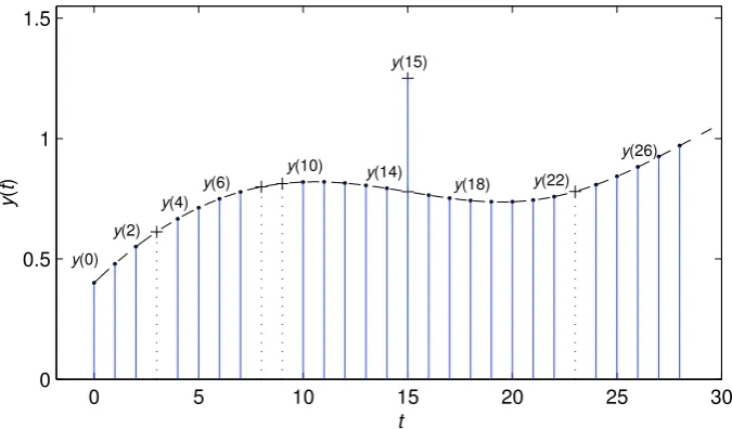
In many applications, there are many reasons for missing sampled-data to arise. In general, a missing-data system implies that most data are available and few data are missing over a period of time. The following considers such a system with missing data that the inputs are normally available at every instant t because the input signals are usually generated by digital computers in practice, and only a small number of data are missing, as shown in Fig. 1 [8, 12], where “+” stands for missing data or bad data (outliers or unbelievable data), e.g., the outputs y(3), y(8), y(9), y(23), . . . are missing samples andy(15),. . .are unbelievable samples.
0 5 10 15 20 25 30
0 0.5 1 1.5
t
y
(
t
)
y(15)
y(0) y(2)
y(4) y(6)
y(10) y(14)
y(18) y(22)
y(26)
Fig. 1 A missing output data pattern
For convenience, we define an integer sequence{ts, s= 0,1,2, . . .}satisfying
0 =t0< t1< t2< t3< . . . < ts−1< ts< . . .
witht∗
s:=ts−ts−1>1, such thaty(t) andϕy(t) are available only whent=ts(s= 0,1,2, . . .), or
equivalently, the data set{y(ts),ϕy(ts) :s= 0,1,2, . . .}contains all available outputs. For instance,
for the missing-data pattern in Fig. 1, when the order na = 3, define the integer sequence {t0,t1, t2, . . ., t9, . . .}, for t0 = 0, t1 = 7, t2 = 13,. . ., t9 = 28,. . ., i.e., {y(t0),ϕy(t0)}, {y(t1),ϕy(t1)},
{y(t2),ϕy(t2)}, . . .,{y(t9),ϕy(t9)},. . . are available.
Replacingtin (4) with tsgives
y(ts) =ϕT(ts)ϑ+v(ts) (33)
with
ϕ(ts) = [ϕTy(ts),ϕxT(ts),φT(ts)]T,
ϕy(ts) = [−y(ts−1),−y(ts−2), . . . ,−y(ts−na)]T,
ϕx(ts) = [−x(ts−1),−x(ts−2), . . . ,−x(ts−nf)]T. (34) 1
[image:7.595.68.406.261.459.2]Consider p data from i = ts−p+1 to i = ts. Define the stacked output vector Y(ts) and the
stacked information matrixΨ(ts) as
Y(ts) :=
y(ts)
y(ts−1)
.. . y(ts−p+1)
∈Rp, Ψ(ts) :=
ϕT(t
s)
ϕT(t
s−1)
.. . ϕT(t
s−p+1)
∈Rp×n
.
Assume that the information vectorϕ(ts) is persistently exciting for largep, that is, [ΨT(ts)Ψ(ts)]
is nonsingular. The difficulty is that the information vectorϕx(ts) inΨ(ts) contains the unknown
variablex(ts−i). Replacingx(ts−i) in (34) with their estimates ˆxk−1(ts−i) at iterationk−1, and
minimizing the quadratic function
J(ϑ) :=kY(ts)−Ψ(ts)ϑk2,
we can obtain the following interval-varying least squares based iterative (V-LSI) algorithm for estimating the parameter vectorϑ:
ˆ
ϑk(ts) = [ ˆΨ
T
k(ts) ˆΨk(ts)]
−1ΨˆT
k(ts)Y(ts), (35)
ˆ
ϑk(t) = ˆϑk(ts), t∈Ts:={ts, ts+ 1, . . . , ts+1−1}, (36)
Y(ts) = [y(ts), y(ts−1), . . . , y(ts−p+1)]T, (37)
ˆ
Ψk(ts) = [ ˆϕk(ts),ϕˆk(ts−1), . . . ,ϕˆk(ts−p+1)]T, (38)
ˆ
ϕk(ts) = [ϕTy(ts),ϕˆTx,k(ts),φT(ts)]T, (39)
ϕy(ts) = [−y(ts−1),−y(ts−2), . . . ,−y(ts−na)]T, (40)
ˆ
ϕx,k(ts) = [−xˆk−1(ts−1),−xˆk−1(ts−2), . . . ,−xˆk−1(ts−nf)]T, (41)
ˆ
ϑk(ts) = [ˆaTk(ts),fˆkT(ts),θˆ
T
k(ts)]T, (42)
ˆ
xk(j) = ˆϕTx,k(j) ˆfk(ts) +φT(j)ˆθk(ts), j∈[t1, ts+1], xˆk(i) = 1/p0, i6t1−1. (43)
We simply hold the parameter estimate ˆϑk(t) remains unchanged over the interval [ts, ts+1−1].
6 The interval-varying D-LSI algorithm
In the following, we study an interval-varying D-LSI algorithm based on the decomposition technique to reduce computational cost.
Replacingtin (14)–(17) withts gives
y1(ts) =y(ts)−ϕTx(ts)f
=ϕT
1(ts)θ1+v(ts),
y2(ts) =y(ts)−ϕT1(ts)θ1
=ϕT
x(ts)f+v(ts).
Define the stacked output vectors Y(ts),Y1(ts) andY2(ts), and the stacked information matrices
Ψ1(ts) andΨx(ts) as
Y(ts) :=
y(ts)
y(ts−1)
.. . y(ts−p+1)
∈Rp, Y1(ts) :=
y1(ts)
y1(ts−1)
.. . y1(ts−p+1)
∈Rp, Y2(ts) :=
y2(ts)
y2(ts−1)
.. . y2(ts−p+1)
∈Rp,
Ψ1(ts) := ϕT
1(ts)
ϕT
1(ts−1) .. . ϕT
1(ts−p+1)
∈Rp×(na+m), Ψ
x(ts) :=
ϕT
x(ts)
ϕT
x(ts−1) .. . ϕT
x(ts−p+1)
∈Rp×nf.
Define two quadratic functions:
J1(θ1) :=kY1(ts)−Ψ1(ts)θ1k2,
J2(f) :=kY2(ts)−Ψx(ts)fk2.
Assume that the information vectors ϕ1(ts) and ϕx(ts) are persistently exciting for large p, that
is, [ΨT
1(ts)Ψ1(ts)] and [ΨTx(ts)Ψx(ts)] are nonsingular. Letting the partial derivatives ofJ1(θ1) and J2(f) with respect toθ1andf be zero leads to the following least squares estimates of the parameter
vectorsθ1 andf:
ˆ
θ1(ts) = [ΨT1(ts)Ψ1(ts)]
−1 ΨT
1(ts)Y1(ts)
= [ΨT
1(ts)Ψ1(ts)]
−1 ΨT
1(ts)[Y(ts)−Ψx(ts)f], (44)
ˆ
f(ts) = [ΨTx(ts)Ψx(ts)]
−1 ΨT
x(ts)Y2(ts)
= [ΨT
x(ts)Ψx(ts)]
−1
ΨT
x(ts)[Y(ts)−Ψ1(ts)θ1]. (45)
However, we can see that the right-hand sides of Equations (44)–(45) contain the unknown param-eters θ1 and f, and the information vectorϕx(ts) inΨx(ts) contains the unknown term x(ts−i),
so the estimates ˆθ1(ts) and ˆf(ts) are impossible to compute directly. Here, we use the hierarchical
identification principle to solve this problem: let ˆθ1,k(ts) :=
ˆ ak(ts)
ˆ θk(ts)
and ˆfk(ts) be the iterative
estimates ofθ1=
a θ
andf at iterationk, respectively, and ˆxk(ts−i) be the estimate ofx(ts−i).
Define
ˆ
ϕx,k(ts) := [−xˆk−1(ts−1),−xˆk−1(ts−2), . . . ,−xˆk−1(ts−nf)]T∈Rnf,
ˆ
Ψx,k(ts) :=
ˆ ϕT
x,k(ts)
ˆ ϕT
x,k(ts−1) .. . ˆ ϕT
x,k(ts−p+1)
∈Rp×nf.
Replacingθ,f andϕx(ts) in (2) with ˆθk(ts), ˆfk(ts) and ˆϕx,k(j), the estimate ˆxk(j) ofx(j) can be
computed by
ˆ
xk(j) = ˆϕTx,k(j) ˆfk(ts) +φT(j)ˆθk(ts).
ReplacingΨx(ts),θ1andf in (44)–(45) with their corresponding estimates ˆΨx,k(ts), ˆθ1,k−1(ts) and
ˆ
fk−1(ts), respectively, we can summarize the interval-varying D-LSI algorithm of computing ˆθ1,k(ts)
and ˆfk(ts) as
ˆ
θ1,k(ts) = [ΨT1(ts)Ψ1(ts)]−1ΨT1(ts)[Y(ts)−Ψˆx,k(ts) ˆfk−1(ts)], (46)
ˆ
θ1,k(t) = ˆθ1,k(ts), t∈Ts:={ts, ts+ 1, . . . , ts+1−1}, (47)
ˆ
fk(ts) = [ ˆΨ
T
x,k(ts) ˆΨx,k(ts)]−1Ψˆ
T
x,k(ts)[Y(ts)−Ψ1(ts)ˆθ1,k−1(ts)], (48)
ˆ
fk(t) = ˆfk(ts), (49)
Y(ts) = [y(ts), y(ts−1), . . . , y(ts−p+1)]T, (50)
Ψ1(ts) = [ϕ1(ts),ϕ1(ts−1), . . . ,ϕ1(ts−p+1)]T, (51)
ˆ
Ψx,k(ts) = [ ˆϕx,k(ts),ϕˆx,k(ts−1), . . . ,ϕˆx,k(ts−p+1)]T, (52)
ϕ1(ts) =
ϕy(ts)
φ(ts)
, (53)
ϕy(ts) = [−y(ts−1),−y(ts−2), . . . ,−y(ts−na)]T, (54)
ˆ
ϕx,k(ts) = [−xˆk−1(ts−1),−xˆk−1(ts−2), . . . ,−xˆk−1(ts−nf)]T, (55)
ˆ
xk(j) = ˆϕTx,k(j) ˆfk(ts) +φT(j)ˆθk(ts), j∈[t1, ts+1−1], (56)
ˆ
θ1,k(ts) =
ˆ ak(ts)
ˆ θk(ts)
, (57)
ˆ
ak(ts) = [ˆa1,k(ts),ˆa2,k(ts), . . . ,aˆna,k(ts)]
T, (58)
ˆ
fk(ts) = [ ˆf1,k(ts),fˆ2,k(ts), . . . ,fˆnf,k(ts)]
T. (59)
To initialize the algorithm, we take ˆθ1,0(t0) and ˆf0(t0) as real vectors with small positive entries,
e.g., ˆθ1,0(t0) = 1na+m/p0, ˆf0(t0) = 1nf/p0, ˆx0(i) = 1/p0 (i 6 t1−1), p0 = 10
6. The parameter
estimates ˆθ1,k(t) and ˆfk(t) in (47) and (49) remain unchanged over the interval [ts, ts+1−1].
The interval-varying D-LSI algorithm (which is abbreviated as the V-D-LSI algorithm) uses the data over the finite data window with the length p, thus the V-D-LSI algorithm can track time-varying parameters and be used for online identification. The interval-varying identification algorithms are proposed for missing-data systems but can be extended to systems with scarce mea-surements.
7 Examples
Example 1 Consider the following linear-in-parameters system: A(z)y(t) = φ
T(t)
F(z)θ+v(t),
A(z) = 1 +a1z−1+a2z−2= 1 + 0.27z−1+ 0.75z−2,
F(z) = 1 +f1z−1+f2z−2= 1−0.31z−10.44z−2,
θ= [b1, b2]T= [−0.56,0.91]T,
ϑ= [a1, a2, f1, f2, b1, b2]T= [0.27,0.75,−0.31,0.44,−0.56,0.91]T.
In simulation, {φ(t)} is taken as an uncorrelated persistent excitation vector sequence with zero mean and unit variance, {v(t)} as a white noise sequence with zero mean and different variances σ2= 0.102andσ2= 0.502, respectively. Take the data lengtht=p=L
e= 3000 data and apply the
LSI algorithm and the D-LSI algorithm to identify this example system, the parameter estimates and their errors δ versus iteration k are shown in Tables 1–2 and Figs. 2–3 where the parameter estimation error is defined as δ:=kϑˆk−ϑk/kϑk ×100%.
From Tables 1–2 and Figs. 2–3, we can draw the following conclusions.
– The estimation errors given by the LSI algorithm and the D-LSI algorithm become smaller (in general) as iterationkincreases or the noise varianceσ2decreases – see Tables 1–2 and Figs. 2–3.
– The parameter estimates given by the LSI algorithm and the D-LSI algorithm are very close to the true parameters for largek – see Tables 1–2.
Table 1 The LSI parameter estimates and errors versus iterationk
σ2 k a
1 a2 f1 f2 b1 b2 δ(%)
0.102 1 0.12130 0.86000 -0.00337 0.00290 -0.56235 0.82223 39.77604
2 0.14538 0.77527 -0.22870 0.29238 -0.56294 0.93341 14.77629 5 0.26612 0.74741 -0.30777 0.43972 -0.55836 0.90819 0.39812 10 0.27048 0.74969 -0.31134 0.44190 -0.55829 0.90758 0.26492 20 0.27048 0.74970 -0.31134 0.44191 -0.55829 0.90758 0.26512 0.502 1 0.13918 0.84802 -0.00655 0.00878 -0.55630 0.80354 39.10793
[image:11.595.72.401.226.540.2]2 0.16413 0.77135 -0.26148 0.29224 -0.55690 0.93013 13.24651 5 0.26898 0.74869 -0.31399 0.44738 -0.55145 0.89849 1.16127 10 0.27235 0.74989 -0.31740 0.44807 -0.55140 0.89829 1.27600 20 0.27234 0.74990 -0.31737 0.44809 -0.55140 0.89828 1.27613 True values 0.27000 0.75000 -0.31000 0.44000 -0.56000 0.91000
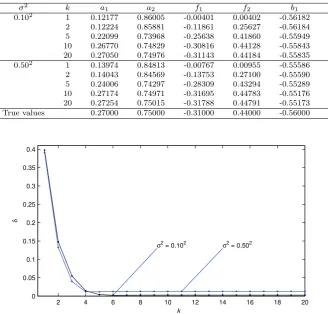
Table 2 The D-LSI parameter estimates and errors versus iterationk
σ2 k a
1 a2 f1 f2 b1 b2 δ(%)
0.102 1 0.12177 0.86005 -0.00401 0.00402 -0.56182 0.82139 39.69414
2 0.12224 0.85881 -0.11861 0.25627 -0.56184 0.82332 23.23453 5 0.22099 0.73968 -0.25638 0.41860 -0.55949 0.88763 5.53938 10 0.26770 0.74829 -0.30816 0.44128 -0.55843 0.90584 0.39957 20 0.27050 0.74976 -0.31143 0.44184 -0.55835 0.90758 0.26330 0.502 1 0.13974 0.84813 -0.00767 0.00955 -0.55586 0.80239 39.03257
2 0.14043 0.84569 -0.13753 0.27100 -0.55590 0.80614 21.44534 5 0.24006 0.74297 -0.28309 0.43294 -0.55289 0.88201 3.51513 10 0.27174 0.74971 -0.31695 0.44783 -0.55176 0.89762 1.27090 20 0.27254 0.75015 -0.31788 0.44791 -0.55173 0.89826 1.27761 True values 0.27000 0.75000 -0.31000 0.44000 -0.56000 0.91000
2 4 6 8 10 12 14 16 18 20
0 0.05 0.1 0.15 0.2 0.25 0.3 0.35 0.4
k
δ
σ2 = 0.502 σ2 = 0.102
Fig. 2 The LSI estimation errors versuskwithσ2= 0.102 andσ2= 0.502
Example 2 Consider the following linear-in-parameters system with missing data: A(z)y(t) = φ
T(t)
F(z)θ+v(t),
A(z) = 1 +a1z−1+a2z−2= 1−1.17z−1+ 0.45z−2,
F(z) = 1 +f1z−1+f2z−2= 1−0.35z−1+ 0.52z−2,
θ= [b1, b2]T= [0.56,0.93]T,
ϑ= [a1, a2, f1, f2, b1, b2]T= [−1.17,0.45,−0.35,0.52,0.56,0.93]T.
The simulation conditions are similar to those of Example 1, here the noise variances σ2 = 0.502
and σ2 = 1.002, respectively. Takes =p =L
e = 3000 and t∗s = 3, collect the input-output data {φ(t), y(ts)}. Apply the V-LSI algorithm and the V-D-LSI algorithm to identify this example system, 1
[image:11.595.67.421.588.702.2]2 4 6 8 10 12 14 16 18 20 0
0.05 0.1 0.15 0.2 0.25 0.3 0.35 0.4
k
δ
σ2 = 0.502 σ2 = 0.102
Fig. 3 The D-LSI estimation errors versuskwithσ2= 0.102andσ2= 0.502
the parameter estimates and their estimation errors δ := kϑˆk(ts)−ϑk/kϑk ×100% versus k are
[image:12.595.90.392.75.248.2]shown in Tables 3–4 and Figs. 4–5.
Table 3 The V-LSI parameter estimates and errors versus iterationk
σ2 k a
1 a2 f1 f2 b1 b2 δ(%)
0.502 1 -1.10186 0.53319 -0.00827 0.00558 0.53791 1.16373 37.75946
2 -1.01136 0.42678 -0.42767 0.25248 0.54744 0.98116 18.37233 5 -1.11555 0.43635 -0.40614 0.43932 0.55198 0.93555 6.40856 10 -1.16423 0.45656 -0.33473 0.48704 0.55060 0.94772 2.39188 15 -1.16632 0.45156 -0.33942 0.51080 0.55093 0.94364 1.23667 20 -1.16497 0.44977 -0.34347 0.51439 0.55107 0.94211 1.01806 1.002 1 -1.11442 0.51426 -0.01346 0.00942 0.53073 1.15876 37.17634
2 -1.11032 0.45120 -0.34239 0.38281 0.54239 0.97659 8.90486 5 -1.15952 0.44729 -0.35694 0.51329 0.54587 0.94197 1.32722 10 -1.16450 0.44895 -0.34075 0.51349 0.54520 0.94783 1.48817 15 -1.16474 0.44887 -0.34008 0.51416 0.54518 0.94804 1.49924 20 -1.16474 0.44885 -0.34008 0.51424 0.54518 0.94803 1.49831 True values -1.17000 0.45000 -0.35000 0.52000 0.56000 0.93000
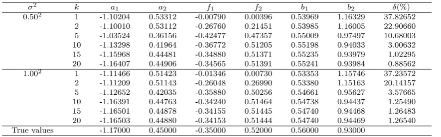
Table 4 The V-D-LSI parameter estimates and errors versus iterationk
σ2 k a1 a2 f1 f2 b1 b2 δ(%)
0.502 1 -1.10204 0.53312 -0.00790 0.00396 0.53969 1.16329 37.82652
2 -1.10010 0.53112 -0.26760 0.21451 0.53985 1.16005 22.90660 5 -1.03524 0.36156 -0.42477 0.47357 0.55009 0.97497 10.68003 10 -1.13298 0.41964 -0.36772 0.51205 0.55198 0.94033 3.00632 15 -1.15968 0.44481 -0.34880 0.51371 0.55235 0.93979 1.02295 20 -1.16407 0.44906 -0.34565 0.51391 0.55241 0.93984 0.88562 1.002 1 -1.11466 0.51423 -0.01346 0.00730 0.53353 1.15746 37.23572
2 -1.11209 0.51143 -0.26048 0.26990 0.53380 1.15163 20.14157 5 -1.12652 0.42035 -0.35880 0.50256 0.54661 0.95627 3.57665 10 -1.16391 0.44763 -0.34240 0.51464 0.54738 0.94437 1.25490 15 -1.16501 0.44878 -0.34155 0.51445 0.54740 0.94468 1.26483 20 -1.16503 0.44880 -0.34153 0.51444 0.54740 0.94469 1.26540 True values -1.17000 0.45000 -0.35000 0.52000 0.56000 0.93000
From Tables 3–4 and Figs. 4–5, it is clear that as the iterationkincreases, the parameter estimates given by the V-LSI algorithm and the V-D-LSI algorithm converge to their true values, and the
[image:12.595.70.512.360.496.2] [image:12.595.70.513.561.699.2]2 4 6 8 10 12 14 16 18 20 0
0.05 0.1 0.15 0.2 0.25 0.3 0.35 0.4
k
δ
σ2 = 1.002 σ2 = 0.502
Fig. 4 The V-LSI estimation errors versuskwithσ2= 0.502andσ2= 1.002
2 4 6 8 10 12 14 16 18 20
0 0.05 0.1 0.15 0.2 0.25 0.3 0.35 0.4
k
δ
σ2 = 1.002 σ2 = 0.502
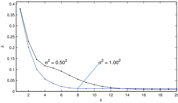
Fig. 5 The V-D-LSI estimation errors versuskwithσ2= 0.502andσ2= 1.002
estimation errors become smaller (generally); under the same data length and noise variance, the estimation accuracies of the V-LSI algorithm and the V-D-LSI algorithm are close.
8 Conclusions
A D-LSI algorithm and a V-D-LSI algorithm are derived for identifying the linear-in-parameters systems by means of the least squares search and the decomposition technique. The analysis shows that under the same noise level and iteration, the D-LSI algorithm and the V-D-LSI algorithm give almost same parameter estimation accuracy. Compared with the LSI algorithm and the V-LSI algorithm, the decomposition based iterative algorithms require less computational cost. The simulation results indicate that the proposed algorithms can generate highly accurate parameter estimates. The identification idea can be extended to study the parameter estimation problems of other linear systems and nonlinear systems with colored noises, missing-data systems and scarce measurement systems [34, 35], hybrid networks and uncertain chaotic delayed systems [20, 21], and can be applied to other fields [15].
[image:13.595.83.379.76.248.2] [image:13.595.83.380.290.463.2]Acknowledgements This work was supported by the National Natural Science Foundation of China (No. 61304138), the Natural Science Foundation of Jiangsu Province (China, BK20130163), the 111 Project (B12018) and the Univer-sity Graduate Scientific Research Innovation Program of Jiangsu Province (SJZZ15 0151).
References
1. M. Amairi, Recursive set-membership parameter estimation using fractional model. Circuits Syst. Signal Process.
34(12), 3757–3788 (2015)
2. H.B. Chen, F. Ding, Y.S. Xiao, Decomposition-based least squares parameter estimation algorithm for input nonlinear systems using the key term separation technique. Nonlinear Dyn.79(3), 2027–2035 (2015)
3. H.B. Chen, Y.S. Xiao, et al., Hierarchical gradient parameter estimation algorithm for Hammerstein nonlinear systems using the key term separation principle. Appl. Math. Comput.247, 1202–1210 (2014)
4. M. Dehghan, M. Hajarian, Iterative algorithms for the generalized centro-symmetric and central anti-symmetric solutions of general coupled matrix equations. Eng. Comput.29(5), 528–560 (2012)
5. F. Ding, System Identification – New Theory and Methods. Beijing: Science Press, 2013.
6. F. Ding, System Identification—Performances Analysis for Identification Methods, Science Press, Beijing, 2014. 7. F. Ding, K.P. Deng, X.M. Liu, Decomposition based Newton iterative identification method for a Hammerstein
nonlinear FIR system with ARMA noise. Circuits Syst. Signal Process.33(9), 2881–2893 (2014)
8. F. Ding, J. Ding, Least squares parameter estimation with irregularly missing data. Int. J. Adapt. Control Signal Process.24(7), 540–553 (2010)
9. J. Ding, C.X. Fan, J.X. Lin, Auxiliary model based parameter estimation for dual-rate output error systems with colored noise. Appl. Math. Model.37(6), 4051–4058 (2013)
10. J. Ding, J.X. Lin, Modified subspace identification for periodically non-uniformly sampled systems by using the lifting technique. Circuits Syst. Signal Process.33(5), 1439-1449 (2014)
11. F. Ding, X.M. Liu, Y. Gu, An auxiliary model based least squares algorithm for a dual-rate state space system with time-delay using the data filtering, Journal of the Franklin Institute – Engineering and Applied Mathematics 353 (2016). doi: 10.1016/j.jfranklin.2015.10.025
12. F. Ding, G. Liu, X.P. Liu, Parameter estimation with scarce measurements. Automatica47(8), 1646–1655 (2011) 13. F. Ding, X.H. Wang, Q.J. Chen, Y.S. Xiao, Recursive least squares parameter estimation for a class of output non-linear systems based on the model decomposition. Circuits Syst. Signal Process.35, (2016). doi: 10.1007/s00034-015-0190-6
14. F. Ding, Y.J. Wang, J. Ding, Recursive least squares parameter estimation algorithms for systems with colored noise using the filtering technique and the auxiliary model. Digit. Signal Process.37, 100-108 (2015)
15. C.L. Fan, H.J. Li, X. Ren, The order recurrence quantification analysis of the characteristics of two-phase flow pattern based on multi-scale decomposition. Trans. Inst. Meas. Control37(6), 793-804 (2015)
16. Y.Q. Hei, W.T. Li, W.H. Fu, X.H. Li, Efficient parallel artificial bee colony algorithm for cooperative spectrum sensing optimization. Circuits Syst. Signal Process.34(11), 3611–3629 (2015)
17. Y.B. Hu, Iterative and recursive least squares estimation algorithms for moving average systems. Simul. Model. Pract. Theory34, 12–19 (2013)
18. Y.B. Hu, B.L. Liu, Q. Zhou, C. Yang, Recursive extended least squares parameter estimation for Wiener nonlinear systems with moving average noises. Circuits Syst. Signal Process.33(2), 655–664 (2014)
19. J. Huang, Y. Shi, H.N. Huang, Z. Li, l-2–l-infinity filtering for multirate nonlinear sampled-data systems using T-S fuzzy models. Digit. Signal Process.23(1), 418–426 (2013)
20. Y. Ji, X.M. Liu, Unified synchronization criteria for hybrid switching-impulsive dynamical networks. Circuits Syst. Signal Process.34(5), 1499-1517 (2015)
21. Y. Ji, X.M. Liu, et al, New criteria for the robust impulsive synchronization of uncertain chaotic delayed nonlinear systems. Nonlinear Dyn.79(1), 1-9 (2015)
22. Q.B. Jin, Z. Wang, X.P. Liu, Auxiliary model-based interval-varying multi-innovation least squares identification for multivariable OE-like systems with scarce measurements. J. Process Control35, 154–168 (2015)
23. Q.B. Jin, Z. Wang, J. Wang, Least squares based iterative identification for multivariable integrating and unstable processes in closed loop. Appl. Math. Comput.242, 10–19 (2014)
24. Q.B. Jin, Z. Wang, Q. Wang, R.G. Yang, Optimal input design for identifying parameters and orders of MIMO systems with initial values. Appl. Math. Comput.224, 735–742 (2013)
25. Q.B. Jin, Z. Wang, R.G. Yang, J. Wang, An effective direct closed loop identification method for linear multi-variable systems with colored noise. J. Process Control24(5), 485–492 (2014)
26. J.H. Li, Parameter estimation for Hammerstein CARARMA systems based on the Newton iteration, Applied Mathematics Letters 26 (1) (2013) 91-96.
27. W.L. Li, Y.M. Jia, J.P. Du, J. Zhang, Robust state estimation for jump Markov linear systems with missing measurements. J. Frankl. Inst.350(6), 1476–1487 (2013)
28. J. Li, J.D. Zhu, Z.H. Feng, Y.J. Zhao, D.H. Li, Passive multipath time delay estimation using MCMC methods. Circuits Syst. Signal Process.34(12), 3897–3913 (2015)
29. X.G. Liu, J. Lu, Least squares based iterative identification for a class of multirate systems. Automatica46(3), 549–554 (2010)
30. H. Raghavan, A.K. Tangirala, R.B. Gopaluni, S.L. Shah, Identification of chemical processes with irregular output sampling. Control Eng. Pract.14(4), 467–480 (2006)
31. C.F. So, S.H. Leung, Maximum likelihood whitening pre-filtered total least squares for resolving closely spaced signals. Circuits Syst. Signal Process.34(8), 2739–2747(2015)
32. Y.J. Wang, F. Ding, Iterative estimation for a nonlinear IIR filter with moving average noise by means of the data filtering technique. IMA J. Math. Control Inf. (2016). doi: 10.1093/imamci/dnv067
33. X.H. Wang, F. Ding, Convergence of the recursive identification algorithms for multivariate pseudo-linear regres-sive systems. Int. J. Adapt. Control Signal Process.30, (2016). doi: 10.1002/acs.2642
34. X.H. Wang, F. Ding, Recursive parameter and state estimation for an input nonlinear state space system using the hierarchical identification principle. Signal Process.117, 208–218 (2015)
35. D.Q. Wang, Y.P. Gao, Recursive maximum likelihood identification method for a multivariable controlled autore-gressive moving average system. IMA J. Math. Control Inf. (2015) doi: 10.1093/imamci/dnv021
36. D.Q. Wang, H.B. Liu, et al., Highly efficient identification methods for dual-rate Hammerstein systems, IEEE Trans. Control Syst. Technol.23(5), 1952-1960 (2015)
37. C. Wang, T. Tang, Several gradient-based iterative estimation algorithms for a class of nonlinear systems using the filtering technique. Nonlinear Dyn.77(3), 769–780 (2014)
38. D.Q. Wang, W. Zhang, Improved least squares identification algorithm for multivariable Hammerstein systems. J. Franklin Inst. – Eng. Appl. Math.352(11), 5292-5370 (2015)
39. L. Xu, The damping iterative parameter identification method for dynamical systems based on the sine signal measurement, Signal Processing 120 (2016) 660-667.
40. L. Xu, A proportional differential control method for a time-delay system using the Taylor expansion approxima-tion, Appl. Math. Computat.236, 391-399 (2014)
41. L. Xu, Application of the Newton iteration algorithm to the parameter estimation for dynamical systems. J. Computat. Appl. Math.288, 33-43 (2015)
42. L. Xu, L. Chen, W.L. Xiong, Parameter estimation and controller design for dynamic systems from the step responses based on the Newton iteration. Nonlinear Dyn.79(3), 2155–2163 (2015)
43. W.G. Zhang, Decomposition based least squares iterative estimation for output error moving average systems. Eng. Comput.31(4), 709–725 (2014)