City, University of London Institutional Repository
Citation
:
Kyriakou, I., Nomikos, N., Pouliasis, P. K. & Papapostolou, N. C. (2016). Affine-Structure Models and the Pricing of Energy Commodity Derivatives. European Financial Management, 22(5), pp. 853-881. doi: 10.1111/eufm.12071This is the accepted version of the paper.
This version of the publication may differ from the final published
version.
Permanent repository link:
http://openaccess.city.ac.uk/12848/Link to published version
:
http://dx.doi.org/10.1111/eufm.12071Copyright and reuse:
City Research Online aims to make research
outputs of City, University of London available to a wider audience.
Copyright and Moral Rights remain with the author(s) and/or copyright
holders. URLs from City Research Online may be freely distributed and
linked to.
Affine-structure models and the pricing of energy
commodity derivatives
Ioannis Kyriakou
1, Nikos K. Nomikos,
Panos K. Pouliasis and Nikos C. Papapostolou
Cass Business School, City University London
106 Bunhill Row, London EC1Y 8TZ, UK
E-mails: [email protected]; [email protected];
p [email protected]; [email protected]
1We thank Gianluca Fusai for fruitful discussions and Russell Gerrard for his valuable
contri-bution that helped improve the paper. Versions of this paper have been presented at the
Cass-ESCP 51st Meeting of the Euro Working Group on Commodities and Financial Modelling, Winter
2014 Conference of the Multinational Finance Society, 4th Energy Finance Christmas Workshop
(EFC14), Energy Finance Seminar (University of Duisburg-Essen, April 2015) and Commodity
Markets Workshop (Oslo, May 2015). We thank R¨udiger Kiesel, Marcel Prokopczuk and other
participants for useful feedback. Usual caveat applies. Correspondence: Ioannis Kyriakou, E-mail:
Abstract
We consider a seasonal mean-reverting model for energy commodity prices with jumps and Heston-type stochastic volatility, as well as three nested models for comparison. By exploiting the affine form of the log-spot models, we develop a general valuation framework for futures and discrete arithmetic Asian options. We investigate five major petroleum commodities from the European market (Brent crude oil, gasoil) and US market (light sweet crude oil, gasoline, heating oil) and analyze the effects of the competing fitted stochastic spot models in futures pricing, Asian options pricing and hedging. We find evidence that price jumps and stochastic volatility are important features of the petroleum price dynamics.
Keywords: energy prices, affine models, futures, arithmetic Asian options, control vari-ate Monte Carlo
1
Introduction
Understanding the stochastic process governing the energy price is essential, owing to the
indispensable role of hydrocarbons in the world economy and the response of macroeconomic
aggregates to oil price shocks. Concerns about the security of energy supply and the influence
of geopolitical events and global economic activity on petroleum prices create the need for
reliable and efficient tools to price energy-related securities and projects.
Energy commodities are predominantly different from conventional financial assets such
as equity and fixed-income securities and, due to intricate price formation mechanisms,
tra-ditional modelling techniques are not directly applicable. For example, seasonal effects arise
naturally from periodic supply and demand patterns1 and have been successfully modelled
by several authors including Routledge et al. (2000) and Borovkova and Geman (2006). In
addition, commodity prices mean-revert to the marginal cost of production; relevant
the-oretical arguments and empirical evidence have been put forward by Bessembinder et al.
(1995), Schwartz and Smith (2000) and Casassus and Collin-Dufresne (2005), among others.
In effect, prices may temporarily be high or low, but will tend toward an equilibrium level.
Furthermore, temporary supply and demand imbalances, changes in market expectations, or
even unanticipated macroeconomic developments may cause sudden jumps in energy prices
(Hilliard and Reis, 1998, Clewlow and Strickland, 2000). Due to construction lags on the
supply side, even a relatively small change in demand can, at times, cause immediate market
movements of large magnitude. Yet, jumps in returns are transient and a more persistent
component may be required. In fact, compared to other markets, energy price volatility is
both relatively higher and more variable over time (see, e.g., Pindyck, 2004). Trolle and
Schwartz (2009) develop a stochastic volatility model for crude oil and highlight its
impor-tance in commodity derivatives pricing. Larsson and Nossman (2011) find that, in addition
1For example, heating oil prices experience an upward pressure during winter when storage capacity
to stochastic volatility, jumps are essential to capture the time series properties of oil prices.
Accounting for both jumps and stochastic volatility provides a reasonable characterization
of energy commodity prices in that it explains the skewness and fat-tail feature of
commod-ity return distributions. Furthermore, it gives rise to realistic implied volatilcommod-ity patterns for
short-term options without also affecting long-term smiles.
The previous discussion encourages the empirical testing of different spot model
specifica-tions for further use as inputs in derivatives pricing and risk management, energy investment
evaluation, asset allocation and planning. The aim of this paper is to conduct a
compre-hensive analysis of stochastic dynamic modelling of European and US petroleum commodity
prices and enrich existing literature with some new insights in several applications such as
futures pricing, options pricing and hedging. In terms of scope our work shares similarities
with recent contributions in the finance literature focused on other markets like, for
exam-ple, the equity index (see Kaeck and Alexander, 2013), freight (see Nomikos et al., 2013)
and real estate (see Fabozzi et al., 2012) markets. More specifically, we consider a seasonal
mean-reverting spot price model with compound Poisson jumps and Heston-type stochastic
volatility, as well as three nested models for comparison: a diffusion with stochastic
volatil-ity, a jump diffusion with constant volatilvolatil-ity, and the classical Schwartz (1997) model with
constant volatility. The Heston (1993) volatility model is both mean-reverting and positive,
accounts for volatility clustering, dependence in increments and realistic implied volatility
patterns. Furthermore, it allows a simple description of the correlation between the driving
noises in the returns and volatility processes; in particular, positive correlation is interpreted
in terms of the so-called inverse leverage effect, i.e., the observation that in commodity
mar-kets large upward price moves are associated with high volatility due to negative relationship
between inventory and prices (e.g., see Pindyck, 2004, Geman, 2005).
The contribution of our paper is three-fold. Firstly, we derive the bivariate characteristic
function of the suggested jump diffusion model with stochastic volatility by solving a system
prices, tackling previously noted (see Benth, 2011) mathematical challenges originated by
the mean-reverting term in the price dynamics in the Heston stochastic volatility framework
and rendering this useful for calibration purposes. Secondly, we fit the models to spot and
futures prices of Brent crude oil and gasoil from the European market and light sweet crude
oil, gasoline and heating oil from the US market. This is the first study to systematically
apply a selection of stochastic models in the particular markets. We find that ignoring jumps
and/or stochastic volatility leads to a less realistic description of the true data-generating
process (DGP). The flexibility of the proposed general model specification is also confirmed
by its ability to accurately fit the observed futures curves in the different markets. The final
line of research that we contribute to in this paper relates to average (Asian) options, whose
terminal payoff depends on the average level of an energy price during a pre-specified time
window (e.g., see Zhang, 1995). These options are very popular in the energy commodity
markets (for example, NYMEX and ICE offer several average price products linked to energy,
e.g., Brent and WTI average price options) as a means of managing price exposure and
potential impact on transactions, due to the time elapsed until a tanker vessel completes
its route from the production site or refinery to its destination. Using our characteristic
function results we obtain closed-form solutions for geometric average options, which we
then use to implement efficient Monte Carlo simulation with control variates to price the
more prevalent discrete arithmetic average options. This way we present a unified pricing
framework under the four models considered, while extending earlier contributions by Kemna
and Vorst (1990) and Fusai and Meucci (2008) based, respectively, on Gaussian and L´evy
log-spot models to members from the more general affine class. The particular technique
provides fast and accurate simulation outcome, which allows us to study the implications of
the assumed spot price dynamics on the Asian option prices. In addition, we set up delta
hedging strategies for the Asian option and investigate their performance under correct
or misspecified hedges with omitted risk factors. We find that the hedging performance
that, under a true DGP encompassing both price jumps and stochastic volatility, which is
corroborated by our analysis, a misspecified hedge that omits the jumps is closest to the true
hedge.
Last but not least, we note that our proposed model framework is of chief relevance to
other markets like, for example, currency and agricultural commodity markets, where the
importance of stochastic volatility and/or jump risk is well-documented (e.g., see Bates,
1996, Ahlip, 2008, Geman and Nguyen, 2005, Brooks and Prokopczuk, 2013). In particular,
Asian options serve as a cheaper alternative to plain vanilla options in hedging, for example,
exposure to a collapse of an exchange rate; or as a means of reducing the exercise of market
power by virtue of the averaging effect, for example, in agricultural commodity markets
where a ‘large player’ can drive the market up or down affecting the payoff of an, otherwise
equivalent, plain vanilla option (see Geman, 2005).
The remainder of this paper is organized as follows. In Section 2 we present our model
assumptions for the dynamics of the spot energy prices. Section 3 provides a description
of the data and the estimation methodology employed. Empirical results are presented in
Section 4. In Section 5 we introduce our valuation framework for discrete arithmetic average
options and apply in pricing and hedging. Section 6 concludes. Mathematical proofs are
deferred to the appendix.
2
Model Specification and Properties
Let (Ω,F, P) be a probability space equipped with filtration F := (Ft)t>0. Define the commodity spot price process S as the sum of a predictable component and a stochastic
component
The predictable component defined by the following sinusoidal function with a linear trend
ft=δ0+δ1sin(2π(t+τ1)) +δ2sin(4π(t+τ2)) +δ3t, (1)
with parameters δ0, δ1, τ1, δ2, τ2, δ3, accounts for deterministic regularities in the spot price
evolution, i.e., seasonal fluctuations and time trend capturing the long-run growth in prices.
Geman (2005) suggests a mean-reverting model framework for commodity spot prices with
stochastic volatility. We adopt the particular model specification and extend this to
accom-modate sudden jumps in the prices, so that the log deseasonalized (and detrended) spot
price X dynamics are given by
dXt=k(ε−Xt)dt+
p
VtdBt+dLt, (2)
where k is the speed at which random shocks dissipate and process X reverts toward level
ε. The evolution of the spot price variance V is modelled by the square-root diffusion as in
Heston (1993), i.e.,
dVt=α(β−Vt)dt+γpVtdWt (3) with positive parameters α (speed of variance mean-reversion), β (long-run mean variance)
and γ (volatility of variance). B and W are correlated standard Brownian motions (i.e.,
E(BtWt) = ρt) allowing possible inverse leverage effect, i.e., high prices associated with high
volatility translating to ρ > 0. The spot price jump arrival is governed by the independent
time-homogeneous compound Poisson process L with constant arrival rate of λ > 0 jumps
(per unit time) of independent and identically normally distributed sizes J withE(J) =: µJ
and Var(J) =:σJ2. Henceforth, we will be using the acronym MRJSV when referring to the
model (2)–(3).
In this study we additionally consider three nested cases of the general model (2)–(3)
MRSV: diffusion model (dLt= 0 for all t) with Heston stochastic volatility.
MRJ: jump diffusion model with constant volatility √Vt =σ for all t.
MR: Schwartz dynamics with dLt = 0 and
√
Vt=σ for all t.
In Sections 3 and 5 we derive futures and option prices based on our proposed model
framework. For this purpose, we require risk neutral dynamics for the spot price. Following
Benth (2011) we employ standard change of measure with respect to the Brownian motion
driving the spot price dynamics
dBt˜ :=dBt+√h
Vt dt,
wherehis the (constant) market price of risk. Note that one may also introduce a change of
measure in the volatility dynamics; we do not consider this here but, instead, as we explain
in Section 3, we calibrate the stochastic volatility model to market prices of traded futures
contracts. A measure-change with respect to the jump process L is also not considered.
MRJSV belongs to the class of affine-structure models (see Duffie et al., 2000 and Duffie
et al., 2003), hence the characteristic function φV,X(t, u1, u2) :=E(exp{iu1Vt+iu2Xt}) has
exponentially affine dependence onV andX, i.e., there exist functionsψ0, ψ1, ψ2 :R+×R2 →
C so that
φV,X(t, u1, u2) = exp{ψJ(t, u2) +ψ0(t, u1, u2) +ψ1(t, u1, u2)V0+ψ2(t, u1, u2)X0}, (4)
where
ψJ(t, u2) :=λt
eiu2µJ−12σ2Ju22 −1
and ψ0, ψ1, ψ2 satisfy the system of Riccati equations
∂ψ2
∂t = −kψ2, (5)
∂ψ1
∂t = −αψ1+ 1 2γ
2ψ2
1 +ργψ1ψ2+
1 2ψ
2
2, (6)
∂ψ0
∂t = αβψ1+k(ε−h/k)ψ2, (7)
subject to the boundary conditions
ψ0(0, u1, u2) = 0, ψ1(0, u1, u2) =iu1, ψ2(0, u1, u2) =iu2.
By straightforward integration of (5) and (7) we get that
ψ2(t, u1, u2) =iu2e−kt (8)
and
ψ0(t, u1, u2) =αβ
Z t
0
ψ1(s, u1, u2)ds+iu2(ε−h/k)(1−e−kt),
respectively. Solving (6) explicitly is not trivial; from Proposition 3 (see Appendix A.1), the
general solution to (6) is given by (A.3)
ψ1(t, u1, u2) = − 2iu2k
γ2 e
−kt
ζ(iu2e−kt) +
M(t, u2)
C(u1, u2)− 12γ2
Rt
0M(s, u2)ds ,
where M is defined in (A.6) and
C(u1, u2) :=
exp−iu2ργ
k + 2
Riu2
0 ζ(y)dy
iu1+ 2iuγ22kζ(iu2)
satisfiesψ1(0, u1, u2) = iu1. Function ζ, which satisfies Eq. (A.1), admits the representation
ζ(y) = X∞ j=1djy
where the coefficients {dj}∞j=1 satisfy the recursion
j+ 1−α−k
k
dj+1 =
Xj−1
i=1didj−i1j>1− ργ
k dj1j>0+ γ2 4k21j=0.
(Alternatively, one may consider solving (6) numerically using, e.g., Matlab built-in solvers,
however, at increased computational cost.)
In the case of the one-dimensional MRJ model with constant volatility σ, the
character-istic function φX(t, u) := E eiuXt
takes the simplified form
φX(t, u) = exp
ψJ(t, u) +iu(ε−h/k)(1−e−kt)− σ2u2
4k (1−e
−2kt
) +iue−ktX0
(9)
(see Cont and Tankov, 2004), whereas in the cases of the MRSV and MR models the
char-acteristic functions of (V, X) andX, respectively, follow directly from (4) and (9) forλ = 0.
3
Data and Estimation Methodology
In this study we consider five energy commodities: two representatives of the European
petroleum market and three from the US market. European spot prices are the dated Brent
(CB), which serves as a benchmark assessment of the price of physical light crude oil in the
North Sea, and the gasoil (GO) European Economic Community Cost in North West Europe;
corresponding futures contracts are traded on the Intercontinental Exchange (ICE Futures
Europe). US spot prices are the light sweet crude oil WTI (CL) at Cushing, Oklahoma,
RBOB gasoline (HU), and No. 2 heating oil (HO) in New York harbor; corresponding
futures are traded on NYMEX of the CME Group. For the purposes of our study we use
a time series of constant-maturity futures; the futures curve is constructed by cubic spline
interpolation of market prices of traded futures contracts. Volume and open interest data
lead us to consider a block of 12 contracts for each commodity from 1 up to 12 months to
at the same point in time avoiding problems related to thin trading, expiration effects and
discontinuities from rolling over futures contracts. We consider a 4-year period from March
12,2009 to March 11,2013, that is, a total of 1,043 daily observations after the necessary
refinements for bank holidays. Data are collected from Datastream.
We use daily historical spot price data to estimate the predictable component (1) for
each commodity. We then employ a two-stage estimation procedure based on Clewlow and
Strickland (2000), Benth (2011) and Broadie et al. (2007). First, using the log deseasonalized
spot price time series, we obtain the spot parameter estimates of the MRJSV and nested
MRSV, MRJ, MR models of Section 2 by recursive filtering. Given these, in the second
stage we use the information embedded in end-of-day futures contract quotes to estimate
the volatility parameters and the market price of risk.
In more details, we define a jump as an observation in the log deseasonalized price changes
series that is greater in absolute value than a market-specific threshold given by a multiple
of the sample standard deviation of the deseasonalized series (see Clewlow and Strickland,
2000). The prices on the identified ‘jump dates’ are substituted by the averages of the
two adjacent prices, the standard deviation of the updated series is recalculated and the
same procedure is repeated until no more jumps are identified2. We then estimate the jump
arrival rateλ by the average number of identified jumps per year; the estimates of the mean
µJ and standard deviation σJ of the jump size distribution are given by the average and
standard deviation of the jump returns, respectively3; parameters k and εof the spot model
are estimated using OLS regression. In order to calibrate the remaining parameters, i.e., the
2We choose the threshold (multiplemof the sample standard deviation) that leads to the best calibrated
model, i.e., the one that minimizes the Jarque and Bera (1980) statistic of the filtered series (ensures that daily log-price changes are closest to the normal distribution). To this end, we implement the jump-removal procedure for different multiples m= 0.5 +k/100,k = 0, . . . ,450, and find that the optimal multiples m∗ are for each market 2.8 (CB), 2.75 (GO), 2.7 (CL), 2.7 (HU) and 2.8 (HO).
3Empirical evidence suggests that the Clewlow–Strickland recursive-filtering approach can be superior
variance model parameters α, β, γ, the correlation coefficient ρ and the market price of risk
h, we use end-of-day futures contract quotes. This is possible given explicit expressions for
the futures price F under the different model specifications.
Proposition 1 The futures price F(0, T) at time 0 for a contract expiring at timeT > 0is given by
F(0, T) = E(ST) = f(T) +E(eXT),
where
E(eXT) =
φV,X(T,0,−i), under MRJSV (and MRSV with λ= 0) φX(T,−i), under MRJ (and MR with λ= 0)
.
Proof. Follows from (4) and (9).
Let Fj,l be the observed futures prices at time tj of a contract maturing at Tl. The
theoretical futures priceFθ(tj, Tl) is given in Proposition 1;Fθ(tj, Tl) depends on the observed
log deseasonalized spot price time series {Xj}nj=1, the unobserved variance series {Vj}nj=1
which we approximate by the (conditional) expected variance{Vˆj}nj=1where ˆVj :=β+( ˆVj−1− β)e−α/264 with unknown ˆV1 to be estimated, and the parameter vectorθ := ( ˆV1, α, β, γ, ρ, h). We obtain θ by minimizing the Euclidean distance between the observed and theoretical
futures prices
θ∗ := arg min θ
Xn
j=1
Xm
l=1
q
|Fj,l−Fθ(tj, Tl)|2, (10)
wherem = 12 is the number of maturities and n= 1,043 the number of days in the sample.
4
Empirical Results
In this section we discuss the estimation results of the four model specifications MRJSV,
MRSV, MRJ and MR for each of the CB, GO, CL, HU and HO markets. We begin the
models in commodity futures pricing. By means of a simulation study, we further examine
if the specified models can accurately represent the true spot price dynamics4.
4.1
Model Calibration
We fit first the predictable component (1) with a trend and two terms capturing annual
and semi-annual seasonal cycles; standard likelihood ratio test leads to acceptance of the
hypothesis of both annual and semi-annual seasonality at the 5% significance level for all
markets. The estimated parameters are reported in Panel A of Table 1 along with their
standard errors. Results suggest that all markets exhibit significant regularities: adjusted
¯
R2 are 76% and 82% for the European CB and GO, and 59%, 79% and 83% for the US CL,
HU and HO.
Next, we employ the estimation procedure described in Section 3. Parameter estimates
with standard errors are reported in Panel B of Table 1. Several remarks are in order.
Parameter k estimates imply that the expected time for the log deseasonalized spot prices
to return half way toward levelε is 51 days (half-lifek−1ln 2), on average, for the European markets (CB and GO) and 35 days for the US markets (CL, HU and HO); inclusion of jumps
in the spot price model results in increased half-lives of 55 and 44 days, respectively, as jump
returns are less persistent. Jumps are infrequent events and tend to be negative. More
specifically, we find that jumps in the European markets are less frequent, i.e., expected
3.2-3.4 jumps per year for GO and CB versus 4.6-5.0 for HO and CL and 7.6 for HU, and
have smaller standard deviation, i.e., 6.4%-6.7% for CB and GO versus 7.7%-7.9% for CL
and HO and 9.2% for HU. The relative importance of the jump component is also evident
by its percentage contribution to the total variance of the fitted spot model, which lies in
4Throughout the paper, we consider the following sample-path generation techniques for the MR, MRSV,
12%-13% for CB and GO, 19%-21% for CL and HO, and 29% for HU.
Turning next to the volatility model parameters, in the case of the MRSV model the
estimated speeds of variance mean-reversion translate to average half-lives (α−1ln 2) of 5.2 (CB and GO) and 3.6 days (CL, HU and HO). In general, the long-run mean variance,
volatility of variance and the correlation between log-prices and variance innovations are
lower for the European CB and GO than for the US CL, HO and HU. We note that the
correlation is found positive in consistency with the inverse leverage effect in energy prices,
meaning that high prices are associated with high volatility, which can be attributed to the
negative relationship between prices and inventory (e.g., see Pindyck, 2004). Incorporating
price jumps (i.e., case of the MRJSV model) has a downward effect on the speed of variance
mean-reversion, long-run mean variance, volatility of variance and correlation level, as the
need for the variance process to create large sudden movements becomes less important.
In addition, we compute the root mean square error (RMSE) and relative RMSE (RRMSE)
of the model-implied theoretical futures prices given in Proposition 1 for each model with
respect to the observed futures prices: RMSE :=
q
1 nm
Pn
j=1
Pm
l=1|Fθ∗(tj, Tl)−Fj,l| 2
and
RRMSE :=
q
1 nm
Pn
j=1
Pm
l=1|Fθ∗(tj, Tl)/Fj,l−1| 2
, where Fj,l is the observed futures prices
at time tj of a contract maturing at Tl, F(tj, Tl) is the theoretical futures price given in
Proposition 1 for each model under the optimal parameter set θ∗ (see Eq. 10), m = 12 (no. of maturities) and n = 1,043 (no. of days in the sample period March 12,2009 to
March 11,2013). Results presented in Panel C of Table 1 suggest that MRJSV generates
lowest pricing error: across markets, average RRMSE is 13% and maximum RRMSE is
16% (HU). (We reach similar conclusion if we consider the mean absolute percentage
er-ror MAPE := 1 nm
Pn
j=1
Pm
l=1|Fθ∗(tj, Tl)/Fj,l−1|; results are currently not presented for brevity.) To test whether any of the extended versions of the basic MR model with price
jumps and/or stochastic volatility yields significant improvement in the futures pricing
per-formance, we apply the Hansen (2005) test5. We find that accurately modelling jumps in the
5We define loss function (LF) differentials between the MR model and each of the MRSV, MRJ and
spot price dynamics improves satisfactorily the fit of the resulting theoretical futures prices
to the observed futures prices compared to the MR model; admitting additionally stochastic
volatility improves the fit further. More specifically, compared to MR, MRJSV provides
a 4% average, across markets, reduction in the RMSE. Unsurprisingly, highest reduction,
that is, 6.3%, is reported in the HU market having the most frequent price jumps, highest
jump size standard deviation, volatility of variance and correlation between variance and
log-price processes. The improvement in the fit brought by MRJSV compared to MRSV
is still high, that is, 2.1% average reduction in the RMSE, whereas compared to MRJ the
RMSE reduction is up to 1%.
We conclude this analysis by referring to an additional error statistic, that is, the mean
percentage error MPE := nm1 Pn j=1
Pm
l=1(Fθ∗(tj, Tl)/Fj,l−1), which we compute for the entire
term structure of futures prices and use to test for systematic bias. The outcome of the test
suggests rejection of this hypothesis at conventional significance levels. For brevity we do
not detail these results here, but we can make these available upon request.
4.2
Simulation Study: True Data-Generating Process
As a next stage in our analysis, we examine whether the proposed models can accurately
represent the true price dynamics of the commodities of interest. Similarly to Kaeck and
Alexander (2013), we compare the model-implied distributions to the empirical one for each
commodity in terms of a set of statistics. We employ the following test procedure: for
each commodity we approximate the empirical distribution of the log-returns using
station-ary bootstrap and construct 90% bootstrap confidence intervals for the standard deviation,
skewness, kurtosis, 1st and 99th percentiles and expected shortfalls at the 1% and 99% levels.
Then, for each model, we simulate 100,000 price paths and log-return sample statistics, and
calculate the percentage number of simulated statistics of a given type falling within the
wherej = 1, . . . , n= 1,043. Then, using 5,000 bootstrap simulations, we test the null hypothesis that MR is not outperformed by the other models, i.e.,H0 :E(LF)≤0. For more details, we refer to White (2000)
corresponding bootstrap confidence interval; a value closer to 1 implies smaller discrepancy
between the observed and assumed price dynamics. The model with the best relative
perfor-mance for given statistic type is indicated by an asterisk in Table 2. If we take a close look
at the table, we see that, although the MR model appears to be fitting well the standard
deviation and the 99th percentile (65% and 89%, respectively, of the time on average across
markets), it naturally does not capture the skewness and kurtosis (33% and 10%,
respec-tively) of the empirical distribution. As a result, the left tail is missed more often in the
case of MR (and MRSV but to a lesser extent). On the other hand, including jumps (i.e.,
case of MRJ and MRJSV models) allows a more balanced and thus accurate fitting of the
tails, adequately accounting for both the skewness and excess kurtosis commonly found in
commodity log-returns. In particular, comparing model-implied standard deviation,
skew-ness and kurtosis across the five markets for each model, we observe that MRJSV produces
more realistic statistics in 10 cases out of 15 (3 statistics × 5 markets). The 1st and 99th
percentiles as well as the expected shortfalls at the 1% and 99% levels of the empirical and
model-implied log-return distributions are also reported suggesting overall superiority of the
MRJSV model in 10 out of 20 cases.
In addition, we employ the two-sample Kolmogorov–Smirnov test with the null hypothesis
stating that the observed and simulated log-return distributions are equal. To this end, for
each of the simulated price paths of the competing models, we test the null hypothesis and
store thep-value. Table 2 reports the percentage number of times the null hypothesis cannot
be rejected at the 10% significance level. In the case of the MR model the null hypothesis
cannot be rejected in 62.1% (CB), 56.5% (GO), 55.1% (CL), 35.7% (HO) and 59.7% (HU) of
the simulation runs. Accounting for price jumps or stochastic volatility (i.e., MRJ or MRSV
model) raises the evidence in favour of the null hypothesis, while the combined effect (i.e.,
case of MRJSV model) is found strongest with non-rejection in 88.4% (CB), 92.8% (GO),
82.1% (CL), 84.4% (HO) and 80.1% (HU) of the time.
more realistic description of the true DGP, accounting for the stylized patterns of the spot
prices in the petroleum markets under consideration.
5
Application on Discrete Arithmetic Asian Options
In what follows we investigate the impact of the proposed stochastic models in Section 2 in
terms of the pricing and delta hedging of options on the discrete arithmetic average spot
price, which are particularly popular in commodity markets. The need for realistic spot price
models capturing the unique characteristics of energy commodities raises substantially the
complexity of the option pricing problem. We solve this by means of an efficient Monte Carlo
simulation approach, which we develop based on the model properties presented in Section
2. We then execute pricing and delta hedging simulation exercises based on the calibrated
model parameters in Section 4.
5.1
Option Pricing
Suppose that the spot price S is monitored over the period [0, T], T > 0, at the following
equidistant dates: 0, δ, . . . , jδ, . . . , nδ =T.
The terminal payoff of the arithmetic Asian option depends on the average of the past
n+ 1 spot prices
1 n+ 1
Xn
j=0Sjδ =An+1+ 1 n+ 1
Xn
j=0fjδ,
where f is given by (1) and
An+1 := 1 n+ 1
Xn
j=0(Sjδ −fjδ) = 1 n+ 1
Xn
j=0e Xjδ
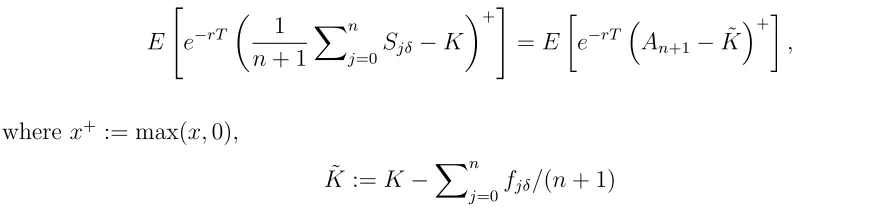
fixed strike price K reads
E
"
e−rT
1 n+ 1
Xn
j=0Sjδ −K
+#
=E
e−rT An+1−K˜
+
, (11)
where x+:= max(x,0),
˜
K :=K−Xn
j=0fjδ/(n+ 1)
is the deseasonalized strike price, andr the continuously compounded risk free rate of
inter-est. Note that the price of the put-type option can be obtained via standard put-call parity.
By analogy, the price of the Asian call option on the geometric average spot price is given
by
E
e−rT
eYn+1 −K˜
+
, (12)
where
Yn+1 := 1 n+ 1
Xn
j=0ln(Sjδ−fjδ) = 1 n+ 1
Xn
j=0Xjδ. (13)
For the purposes of our analysis, we estimate the price of the arithmetic option, i.e.,
evaluate (11), by employing an accurate control variate Monte Carlo (CVMC) scheme with
[image:19.612.71.513.103.208.2]100,000 simulations and the geometric Asian option price (12) used as control variate (see
Table 3 and Glasserman, 2004 for more details). Given the exact closed-form expression for
the price of the geometric option under Black–Scholes–Merton model assumptions, Kemna
and Vorst (1990) show that the geometric option serves as an efficient control variate in
the simulation of the arithmetic option. Fusai and Meucci (2008) extend to L´evy log-spot
models by adopting a Fourier transform approach, whereas in this paper we generalize to
non-L´evy members of the affine class, including the MRJSV model and the nested models
of Section 2. To this end, we derive first the characteristic function of the log-geometric
average, φYn+1(u) :=E(exp{iuYn+1}), under the given model assumptions.
(a) under the MRJSV model dynamics by
φYn+1(u) = exp
nXn
j=1(ψJ(δ, ϑj) +ψ0(δ, ηj, ϑj)) +ψ1(δ, η1, ϑ1)V0+iϑ0X0
o
, (14)
whereηn:= 0, ϑn :=u/(n+1),ηj :=−iψ1(δ, ηj+1, ϑj+1)andϑj :=−iψ2(δ, ηj+1, ϑj+1)+ u/(n+ 1) for 0≤j ≤n−1.
(b) under the MRJ model dynamics by
φYn+1(u) =
Yn
j=0exp
iu n+ 1X0e
−kjδ
×Yn
j=1exp
ψJ(δ, ηj) +iηj(ε−h/k)(1−e−kδ)− σ2η2
j 4k (1−e
−2kδ )
,
where ηj :=uPn
−j m=0e
−mkδ/(n+ 1) for 0< j ≤n.
Relevant results under the MRSV and MR models follow directly by setting λ= 0.
Proof. See Appendix A.2.
Given the characteristic function of the log-geometric average, the exact price of the
geometric Asian option (12) can be computed by means of the Fourier-inversion formula
with respect to the log-strike price ˜κ:= ln ˜K
E
e−rT eYn+1−K˜
+
= e
−ξκ˜−rT 2π
Z
R
e−iuκ˜ φYn+1(u−ξi−i)
(iu+ξ)(iu+ξ+ 1)du, (15)
where constant ξ > 0 ensures integrability in ˜κ (see Carr and Madan, 1999). Formula (15)
can be evaluated using the (fractional) fast Fourier transform algorithm (e.g., fftorcztin
Matlab, see ˇCern´y and Kyriakou, 2011 for more details) which outputs the geometric Asian
option prices on a fine, equally spaced grid of log-strike prices.
Based on the estimated model parameters (see Table 1) and using our results for the
geometric Asian option, we implement standard CVMC setup (see Table 3) to estimate the
to maturity arithmetic Asian call options with daily monitoring (i.e., n= 22). In particular,
the strike price is set equal to 100%, 95% and 105% of the spot price. The current spot
price and variance are set equal to exp(ε) andβ, respectively, and the risk free interest rate
is given by the average 3-month US T-bill rate throughout the sample period. Computed
option prices are presented in Table 4 in monetary terms (CB $/bbl, GO $/mt, CL
-$/bbl, HU - c$/gal, HO - c$/gal) as well as relative to the spot price and the price of the
corresponding ATM option.
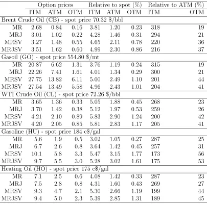
Results suggest that ignoring jumps and stochastic volatility leads to lower option prices.
More specifically, we find that, across all markets, MRSV and MRJSV prices are
system-atically higher than the corresponding MRJ prices, which, further, are higher than the MR
ones. In fact, the discrepancies between MRSV, MRJSV and MRJ prices versus MR prices
are higher for in-the-money options, whereas these reduce the more out-of-the-money the
option. Our observation based on option prices under non-L´evy (i.e., dependent) log-returns
adds to earlier contributions by Fusai and Meucci (2008) and ˇCern´y and Kyriakou (2011),
who observe similar pattern across different level of moneyness based on option prices
rely-ing on L´evy (i.e., independent) assumptions for stock log-returns. As noted in ˇCern´y and
Kyriakou (2011), such pattern is attributed to the combined kurtosis-skewness effect in a
L´evy and non-L´evy, as opposed to normal, log-return distribution.
5.2
Hedge Performance Comparisons
The MRJ, MRSV and MRJSV models we have considered in this paper generally correspond
to incomplete markets due to the presence of stochastic jumps and/or volatility, thus
intro-ducing a hedging error in a delta hedging strategy even in the theoretical limit of continuous
rebalancing as the two instruments (the underlying and the risk free bond) are not enough to
span the sources of uncertainty. In the case of the one-factor MR diffusion, existence of error
can be attributed to the discreteness of the portfolio rebalancing frequency. In what follows,
options and inspect the performance of the delta hedge in the various markets. We define
the hedging error as the difference between the value of the daily-rebalanced hedge portfolio
and the value of a 1-month to maturity, daily-averaged ATM arithmetic Asian option for a
1-week hedge period.
We use Monte Carlo simulation to gauge the magnitude and distributional characteristics
of the hedging error. For each commodity we simulate the distribution of the hedging
error when the underlying data-generating process is given by either of the MR, MRJ,
MRSV and MRJSV models and (a) the hedge portfolios are formed accordingly, or (b)
the hedge portfolios are misspecified, i.e., are formed based on alternative models. In fact,
case (b) is more realistic as the hedger never really knows the true DGP, hence develops the
hedging approach based on some assumptions. The particular task allows us to investigate
the sensitivity of the hedging performance to model misspecification, in other words, the
impact of incorrectly specifying the underlying data-generating process and forming the
hedge portfolios. In simulating the hedging error distributions under the dynamic strategy,
the option prices are estimated daily using the CVMC approach in Section 5.1, whereas the
option deltas using a modified version based on straightforward application of the pathwise
technique (see Glasserman, 2004) with the geometric Asian option delta used as control
variate.
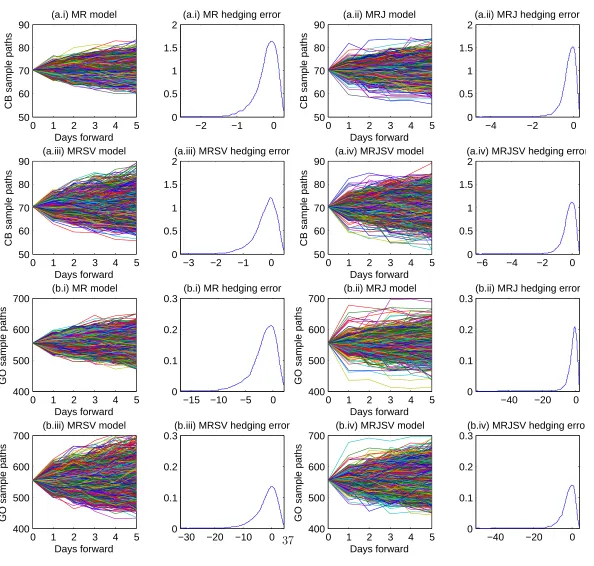
We consider first computed hedging errors under each driving process with the hedge
portfolios formed accordingly. Figure 1 plots the simulated price paths of each underlying
commodity across the 5-day hedge period coupled with the hedging error distributions at the
closing of the week-long hedging exercise, under the four data-generating processes. Most
of the hedging errors are negative, irrespective of the direction of the moves in the price
of the underlying. As discussed in Carr and Wu (2014), the reason is that the option price
exhibits convexity with the price of the underlying, resulting in the value of the delta neutral
portfolio being below the value of the option contract under sufficiently large price
when jumps are allowed, and therefore larger moves in the price of the underlying, as in our
MRJ and MRJSV models. Our results are consistent with those of Carr and Wu (2014) in
the sense of achieving negative skewness of hedging error and positive excess kurtosis, even
in the case of the underlying price moving purely diffusively; as shown in Figure 1, this effect
becomes more perceptible when discontinuities are allowed in the price dynamics. This also
explains the negative mean hedging error reported in Panel A of Table 5 across all markets
and models (see also Brooks and Prokopczuk, 2013 for the case of European options),
al-though expectedly this is smaller (in absolute value) in the case of the pure diffusion model.
Models with jumps and/or stochastic volatility generate hedging errors with increased
stan-dard deviation compared to the basic one-factor model. Therefore, the performance of the
delta hedge deteriorates when more than one risk factors are allowed.
In the event of model misspecification, the investor’s hedge model deviates from the true
model. Panel B of Table 5 reports the percentage changes in the standard deviation of the
hedging error under different misspecified hedge portfolios, allowing us to explore the effect
of model uncertainty on the hedging error. More specifically, we consider incorrect hedges
containing fewer risk factors than the true model, i.e., the misspecified hedge model either
omits the jump component, the stochastic volatility, or both. Incorrect hedges in this case
always result in increased standard deviation of the hedging error (positive entries in Panel
B). When the MRJSV model represents the true DGP (Panel B.3), as also corroborated
by our analysis in Section 4, we find that the misspecified MRSV hedge performs better
achieving lowest increase of standard deviation in the GO, CL, HU and HO markets, the CB
market being the only exception in which case the MRJ hedge is slightly better. Therefore,
we find that the hedge model with stochastic volatility is closest to the true hedge. Our
observation is consistent with the remarks of Branger et al. (2012) based on the analysis of
different hedging strategies for plain vanilla stock options. It is worth noting that we do
not consider the opposite situation, i.e., hedge models with more risk factors than the true
complicated and involves many risk factors while investors are simpler than ‘real life’ (see
Branger et al., 2012).
Finally, we perform a robustness check of the outcome of the hedging exercise. We
per-turb each of the parameters by ±1% from their original estimates and study the impact
on the variance of the hedging error. Through this sensitivity analysis, we reach that the
signs of the entries in Table 5 remain unchanged. Further research toward this direction
could include, for example, a study of the distribution of the variance (and possibly higher
moments) of the hedging error under parameter resampling; this is a nontrivial and
partic-ularly computationally intensive problem at this stage, due to the extremely large number
of simulations required, whose further investigation is left for future research.
6
Summary and Conclusion
We have considered five major European and US petroleum commodity markets to study
the ability of four different model specifications to realistically portray the dynamics of
the data-generating process using historical spot and futures price data over the period
March 2009 to March 2013. Our selection of models includes a seasonal mean-reverting
spot price model with jumps and Heston-type stochastic volatility (MRJSV) and nested
specifications with/out jumps or stochastic volatility (MR, MRJ, MRSV). In the first stage
of our analysis, we assess relative performance by comparing simulated model-implied and
empirically estimated statistics as well as testing for equality of the observed and simulated
log-return distributions; our exercise indicates superior performance of the MRJSV model
in producing dynamics that are similar to the true price dynamics. Furthermore, using
the theoretical futures prices derived for all competing models, we investigate the fit to the
observed futures curves in the different markets; our error statistics point toward inclusion
of price jumps, while combining with stochastic price volatility improves the fit further.
In addition, given the widespread use of Asian options in commodity markets, we provide
monitoring when the underlying spot is driven by a general exponential affine model. Our
findings suggest that failing to account for price jumps and stochastic volatility leads to
relatively lower option premia, especially for in-the-money call options. Furthermore, we
gauge the distributional characteristics of the hedging error from dynamic delta hedging
strategies applied to an Asian option. In the case of an investor with perfect knowledge of
the stochastic process governing the underlying asset price, the performance of the hedging
strategy deteriorates in the presence of random price jumps and/or volatility. The delta
hedge becomes even more ineffective in the case of incorrectly specified hedges with omitted
risk factors. We find that when the MRJSV model represents the true DGP, as corroborated
by our analysis in Section 4, a misspecified hedge with omitted jumps but allowed stochastic
volatility is closest to the true hedge.
The implications of this research are of chief relevance to market participants, as
spec-ifying correctly the dynamic behaviour of the underlying spot price process is important
for understanding and managing the risks associated with derivative securities, investment
evaluation, asset allocation and planning.
Appendix A:
Proofs
A.1
Proof of general solution to Riccati equation (6)
Proposition 3 Suppose ζ(y), y∈C\{0}, satisfies the equation
ζ0(y) =ζ(y)2+
α−k ky −
ργ k
ζ(y) + γ 2
4k2. (A.1)
Define
χ(t, u2) = − 2iu2k
γ2 e
−ktζ(iu
2e−kt). (A.2)
Then,
(b) the general solution to (6) takes the form
ψ1 =χ+ 1
w, (A.3)
where w satisfies the differential equation
∂w
∂t + −α+iu2ργe
−kt+γ2χ
w=−1
2γ
2. (A.4)
Proof.
(a) From (A.2), we obtain
∂χ
∂t = −kχ− 2u22k2
γ2 e
−2ktζ0
(iu2e−kt)
= −kχ− 2u
2
2k2
γ2 e
−2kt
ζ(iu2e−kt)2+
α−k iu2ke−kt
− ργ
k
ζ(iu2e−kt) + γ2 4k2
= −αχ+1 2γ
2χ2+ργχψ
2 +
1 2ψ
2
2, (A.5)
where the second equality follows from (A.1) and ψ2 in the last equality is given by
(8). It is implied from (A.5) that χ is a solution to (6).
(b) Suppose that χ+ 1/w is an arbitrary solution to (6). Then we have
∂χ ∂t −
1 w2
∂w
∂t =−α
χ+ 1 w +1 2γ 2
χ2+ 2χ w + 1 w2 +ργ
χ+ 1 w
ψ2+ 1 2ψ
2 2
and, further, from (A.5) we get
− 1
w2 ∂w
∂t =− α w + 1 2γ 2 2χ w + 1 w2
+ργψ2 w ,
For the differential equation (A.4) with χ given in (A.2), from standard calculus theory
the integrating factor is
M(t) := exp
−αt− iu2ργ
k e
−kt−2iu
2k
Z
e−ktζ(iu2e−kt)dt
= exp −αt− iu2ργ
k e
−kt+ 2
Z iu2e−kt
0
ζ(y)dy
!
, (A.6)
from which we get the general solution to (A.4)
w(t) = C− 1
2γ
2Rt
0M(s)ds M(t)
where C is the constant of integration.
A.2
Proof of Proposition 2
Proof.
(a) Under the MRJSV model dynamics, we have from (4) that
E exp{iηnVnδ +iϑnXnδ} |F(n−1)δ
= expψJ(δ, ϑn) +ψ0(δ, ηn, ϑn) +ψ1(δ, ηn, ϑn)V(n−1)δ+ψ2(δ, ηn, ϑn)X(n−1)δ(A.7),
and for j =n−1, n−2, . . . ,1
E
exp
ψ1(δ, ηj+1, ϑj+1)Vjδ +
ψ2(δ, ηj+1, ϑj+1) + iu n+ 1
Xjδ
F(j−1)δ
= expψJ(δ, ϑj) +ψ0(δ, ηj, ϑj) +ψ1(δ, ηj, ϑj)V(j−1)δ+ψ2(δ, ηj, ϑj)X(j−1)δ .(A.8)
Evaluating
E eiuYn+1=E
exp
iu n+ 1
Xn
j=0Xjδ
(b) Define Zj = Xjδ − X(j−1)δe−kδ, where j = 1, . . . , n. By recursive substitution in Xjδ =X(j−1)δe−kδ+Zj and summation across all j, we get
Xn
j=0Xjδ =X0+
Xn
j=1
n
X0e−kjδ+
Xn−j
m=0Zje
−mkδo.
Then,
E eiuYn+1 = E
exp
iu n+ 1
Xn
j=0Xjδ
= exp
iu n+ 1
Xn
j=0X0e
−kjδ
E
exp
iu n+ 1
Xn
j=1Zj
Xn−j
m=0e
−mkδ
= Yn j=0exp
iu n+ 1X0e
−kjδ
Yn
j=1E(exp{iηjZj}),
where the last equality follows by stochastic independence of the variables{Zj}n j=1 and the characteristic function of Zj from Eq. (9).
References
Ahlip, R., ‘Foreign exchange options under stochastic volatility and stochastic interest rates’,
International Journal of Theoretical and Applied Finance, Vol. 11(3), 2008, pp. 277–294.
Andersen, L., ‘Simple and efficient simulation of the Heston stochastic volatility model’,
Journal of Computational Finance, Vol. 11(3), 2008, pp. 1–42.
Bates, D.S., ‘Jumps and stochastic volatility: exchange rate processes implicit in deutsche
mark options’, Review of Financial Studies, Vol. 9(1), 1996, pp. 69–107.
Benth, F.E., ‘The stochastic volatility model of Barndorff-Nielsen and Shephard in
Bessembinder, H., Coughenour, J.F., Seguin, P.J. and Smoller, M.M., ‘Mean reversion in
equilibrium asset prices: evidence from the futures term structure’, Journal of Finance, Vol. 50(1), 1995, pp. 361–375.
Borovkova, S. and Geman, H., ‘Seasonal and stochastic effects in commodity forward curves’,
Review of Derivatives Research, Vol. 9(2), 2006, pp. 167–186.
Borovkova, S. and Permana, F., ‘Modelling electricity prices by the potential jump-diffusion’,
in A. N. Shiryaev, M. R. Grossinho, P. E. Oliveira, M. L. Esqu´ıvel, eds.,Stochastic Finance (New York: Springer, 2006), pp. 239–263.
Branger, N., Krautheim, E., Schlag, C. and Seeger, N., ‘Hedging under model
misspecifica-tion: all risk factors are equal, but some are more equal than others...’, Journal of Futures Markets, Vol. 32(5), 2012, pp. 397–430.
Broadie, M., Chernov, M. and Johannes, M., ‘Model specification and risk premia: Evidence
from futures options’, Journal of Finance, Vol. 62(3), 2007, pp. 1453–1490.
Brooks, C. and Prokopczuk, M., ‘The dynamics of commodity prices’, Quantitative Finance, Vol. 13(4), 2013, pp. 527–542.
Carr, P. and Madan, D.B., ‘Option valuation using the fast Fourier transform’, Journal of Computational Finance, Vol. 2(4), 1999, pp. 61–73.
Carr, P. and Wu, L., ‘Static hedging of standard options’,Journal of Financial Econometrics, Vol. 12(1), 2014, pp. 3–46.
Casassus, J. and Collin-Dufresne, P., ‘Stochastic convenience yield implied from commodity
futures and interest rates’, Journal of Finance, Vol. 60(5), 2005, pp. 2283–2331.
ˇ
Cern´y, A. and Kyriakou, I., ‘An improved convolution algorithm for discretely sampled
Clewlow, L. and Strickland, C., Energy Derivatives: Pricing and Risk Management (London: Lacima Publications, 2000).
Cont, R. and Tankov, P., Financial Modelling with Jump Processes (Boca Raton: Chapman & Hall/CRC Press, 2004).
Duffie, D., Filipovi´c, D. and Schachermayer, W., ‘Affine processes and applications in
fi-nance’, The Annals of Applied Probability, Vol. 13(3), 2003, pp. 984–1053.
Duffie, D., Pan, J. and Singleton, K., ‘Transform analysis and asset pricing for affine
jump-diffusions’, Econometrica, Vol. 68(6), 2000, pp. 1343–1376.
Fabozzi, F.J., Shiller, R.J. and Tunaru, R.S., ‘A pricing framework for real estate derivatives’,
European Financial Management, Vol. 18(5), 2012, pp. 762–789.
Fusai, G. and Meucci, A., ‘Pricing discretely monitored Asian options under L´evy processes’,
Journal of Banking & Finance, Vol. 32(10), 2008, pp. 2076–2088.
Geman, H., Commodities and Commodity Derivatives: Modeling and Pricing for Agricul-turals, Metals and Energy (Chichester: Wiley-Finance, 2005).
Geman, H. and Nguyen, V.N., ‘Soybean inventory and forward curve dynamics’, Manage-ment Science, Vol. 51(7), 2005, pp. 1076–1091.
Geman, H. and Roncoroni, A., ‘Understanding the fine structure of electricity prices’, The Journal of Business, Vol. 79(3), 2006, pp. 1225–1261.
Glasserman, P.,Monte Carlo Methods in Financial Engineering (New York: Springer, 2004).
Hansen, P.R., ‘A test for superior predictive ability’, Journal of Business & Economic Statistics, Vol. 23(4), 2005, pp. 365–380.
Heston, S.L., ‘A closed-form solution for options with stochastic volatility with applications
Hilliard, J.E. and Reis, J., ‘Valuation of commodity futures and options under stochastic
convenience yields, interest rates, and jump diffusions in the spot’, Journal of Financial and Quantitative Analysis, Vol. 33(1), 1998, pp. 61–86.
Jarque, C.M. and Bera, A.K., ‘Efficient tests for normality, homoscedasticity and serial
independence of regression residuals’, Economics Letters, Vol. 6(3), 1980, pp. 255–259.
Kaeck, A. and Alexander, C., ‘Stochastic volatility jump-diffusions for European equity
index dynamics’, European Financial Management, Vol. 19(3), 2013, pp. 470–496.
Kemna, A.G.Z. and Vorst, A.C.F., ‘A pricing method for options based on average asset
values’, Journal of Banking & Finance, Vol. 14(1), 1990, pp. 113–129.
Larsson, K. and Nossman, M., ‘Jumps and stochastic volatility in oil prices: Time series
evidence’, Energy Economics, Vol. 33(3), 2011, pp. 504–514.
Nomikos, N. and Andriosopoulos, K., ‘Modelling energy spot prices: Empirical evidence
from NYMEX’, Energy Economics, Vol. 34(4), 2012, pp. 1153–1169.
Nomikos, N.K., Kyriakou, I., Papapostolou, N.C. and Pouliasis, P.K., ‘Freight options:
Price modelling and empirical analysis’, Transportation Research Part E: Logistics and Transportation Review, Vol. 51, 2013, pp. 82–94.
Pindyck, R.S., ‘Volatility and commodity price dynamics’, Journal of Futures Markets, Vol. 24(11), 2004, pp. 1029–1047.
Politis, D.N. and Romano, J.P., ‘The stationary bootstrap’, Journal of the American Statistical Association, Vol. 89(428), 1994, pp. 1303–1313.
Routledge, B.R., Seppi, D.J. and Spatt, C.S., ‘Equilibrium forward curves for commodities’,
Journal of Finance, Vol. 55(3), 2000, pp. 1297–1338.
Schwartz, E. and Smith, J.E., ‘Short-term variations and long-term dynamics in commodity
Schwartz, E.S., ‘The stochastic behaviour of commodity prices: implications for valuation
and hedging’, Journal of Finance, Vol. 52(3), 1997, pp. 923–973.
Sullivan, R., Timmermann, A. and White, H., ‘Data-snooping, technical trading rule
per-formance, and the bootstrap’, Journal of Finance, Vol. 54(5), 1999, pp. 1647–1691.
Trolle, A.B. and Schwartz, E.S., ‘Unspanned stochastic volatility and the pricing of
com-modity derivatives’, Review of Financial Studies, Vol. 22(11), 2009, pp. 4423–4461.
White, H., ‘A reality check for data snooping’, Econometrica, Vol. 68(5), 2000, pp. 1097– 1126.
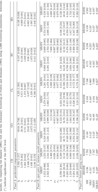
T able 1: Mo del calibration This table presen ts the mo del calibration results. P anel A rep orts the estimated ann ualized parameters (s tan dard errors in [ ]) of the predictable comp onen t (1) for eac h of the Bren t Crude Oil (CB), Gasoil (GO), WTI Crude Oil (CL), Gasoline (HU) and Heating Oil (HO) mark ets (note that parameter δ0 is estimated sub ject to min( St − ft ) = min St to ensure p ositiv e St − ft ). P anel B re p orts the estimated ann ualized parameters (standard e rrors in [ ]) of the MRSV and MRJSV m o dels. P anel C rep orts the e rror statistics computed for the en tire term structure of futures pr ic es: RRMSE := q 1 mn P
n j=1
P
m l=1
| Fθ ∗ ( tj , Tl ) /F j ,l − 1 | 2 and RMSE := q 1 mn P
n j=1
P
m l=1
[image:33.612.205.543.70.730.2]| Fθ ∗ ( tj , Tl ) − Fj ,l | 2 , where Fj ,l is the observ ed futures prices at time tj of a con tract m atu ring at Tl , Fθ ∗( tj , Tl ) is the theoretical futures price giv en in P rop osition 1 for eac h mo del under optimal parameter set θ ∗ (see Eq. 10), m = 12 (no. of maturities) an d n = 1 , 043 (no. of da ys in sample p erio d Marc h 12, 2009 to Marc h 11, 2013). In addition, w e test the n ull h y p othesis th at none of MRJ, MRSV and MRJS V mo dels leads to reduction in futures pricing errors (RRMSE and RMSE) relativ e to the MR mo del, b y emplo yi ng the Hanse n (2005) test and th e stationary b o otstrap of P olitis and Romano (1994) using 5,000 b o otstrap sim ulations. Asterisks ( ∗ ) indicate significance at the 10% lev el. CB GO CL HU HO P anel A: predictable comp onen t parameters δ0 –5.592 [1.217] –40.64 [8.740] –4.235 [1.305] –0.187 [0.029] –0.136 [0.0 38] δ1 3.479 [0.362] –20.56 [2.021] 3.871 [0.480] 0.156 [0.001] –0.069 [0.001 ] τ1 1.204 [0.042] 3.711 [0.055] 1.273 [0.06 7] 1.059 [0.020] 0.774 [0.011] δ2 –2.406 [0.751] –23.62 [0.403] –0.877 [2.582] 0.06 [0.001] 0.062 [0.0 01] τ2 1.836 [0.031] –2.673 [0.024] 1.328 [0.101] 1.073 [0.028] 1.085 [0.067] δ3 14.86 [0.576] 141.2 [4.339] 8.566 [0.91 4] 0.411 [0.012] 0.446 [0.021] P anel B: sp ot price & v ariance mo del parameters MRSV MRJSV MRSV MRJSV MRSV MRJSV MRSV MRJSV MRSV MRJSV ε 4.252 [0.066] 4.253 [0.137] 6.318 [0.056] 6.319 [0.062] 4.279 [0.034] 4.281 [0.041] 0.608 [0.037] 0.609 [0.085] 0 .554 [0.043] 0.559 [0 .058] k 3.563 [0.423] 3.344 [0.206] 3.281 [1.413] 2.999 [0.680] 5.002 [1.775] 4.278 [0.117] 6.385 [2.018] 4.703 [1.034] 4 .088 [1.505] 3.221 [1 .503] λ -3. 400 [0.751] -3.2 [0.540] -5.000 [0.5 26] -7.6 00 [1.064] -4.600 [0.417] µJ -–0.026 [0.016] -–0.013 [0.017] -–0.002 [0.0 15] -–0.007 [0.015] -–0.002 [0.016] σJ -0. 064 [0.001] -0.067 [0.002] -0.077 [0.002] -0.092 [0.002] -0.079 [0.002] h 0.599 [0.301] 0.389 [0.206] 0.643 [0.200] 0.533 [0.184] 0.223 [0.032] 0.215 [0.028] 1.101 [0.323] 0.983 [0.285] 0 .546 [0.244] 0.530 [0 .240] α 36.68 [20.34] 31.52 [18.34] 30.71 [3.442] 16.76 [3.014] 37.33 [19.96] 21.920 [12.89] 84.23 [43.01] 52.32 [24.21] 42.12 [19.87] 40.33 [14.62] β 0.263 [0.064] 0.230 [0.062] 0.349 [0.070] 0.245 [0.052] 0.315 [0.100] 0.216 [0.062] 0.700 [0.101] 0.478 [0.085] 0 .350 [0.100] 0.344 [0 .069] γ 1.259 [0.600] 0.989 [0.546] 1.860 [1.090] 1.084 [0.633] 1.531 [0.770] 1.114 [0.633] 3.694 [2.001] 1.950 [1.109] 1 .817 [1.055] 1.742 [1 .033] ρ 0.204 [0.211] 0.181 [0.226] 0.254 [0.224] 0.186 [0.167] 0.236 [0.212] 0.172 [0.177] 0.452 [0.602] 0.300 [0.326] 0 .247 [0.268] 0.245 [0 .242]
ˆV1
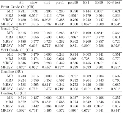
Table 2: True data-generating process testing
We test whether the proposed models (MR, MRJ, MRSV, MRJSV) can accurately represent the true price
dynamics of each commodity (CB, GO, CL, HU, HO). The table reports the relative performance across models in terms of percentage number of simulated log-return statistics of a given type lying within the
corresponding 90% bootstrap confidence interval of the empirical statistic. Table entries correspond to
values in the range 0 to 1: e.g., a value of 0.750 indicates that in 75% of 100,000 simulation runs, the simulated statistic has been within the bootstrap confidence interval. Abbreviations: standard deviation
(std), skewness (skew), kurtosis (kurt), 1st and 99th percentiles (perc1 and perc99) and expected shortfalls
at the 1% and 99% levels (ES1 and ES99). In addition, for each simulation, we employ the two-sample Kolmogorov–Smirnov (K–S) test for equality of the empirical and model-implied log-return distributions
and report the percentage number of times the null hypothesis cannot be rejected at the 10% significance
level. Asterisks (∗) highlight best relative performance across models.
std skew kurt perc1 perc99 ES1 ES99 K–S test Brent Crude Oil (CB)
MR 0.731 0.031 0.295 0.280 0.890 0.144 0.803∗ 0.621 MRJ 0.866 0.556∗ 0.513 0.708 0.951∗ 0.779 0.564 0.833 MRSV 0.789 0.223 0.963∗ 0.388 0.766 0.242 0.747 0.646 MRJSV 0.871∗ 0.515 0.787 0.744∗ 0.860 0.857∗ 0.509 0.884∗ Gasoil (GO)
MR 0.575 0.122 0.189 0.263 0.817 0.109 0.881∗ 0.565 MRJ 0.896∗ 0.556 0.530 0.608 0.937∗ 0.777 0.772 0.811 MRSV 0.788 0.577 0.720 0.282 0.862 0.266 0.857 0.724 MRJSV 0.767 0.606∗ 0.772∗ 0.696∗ 0.821 0.800∗ 0.786 0.928∗ WTI Crude Oil (CL)
MR 0.679 0.479 0.000 0.243 0.834 0.003 0.341 0.551 MRJ 0.855 0.474 0.222 0.621 0.868∗ 0.728∗ 0.763 0.770 MRSV 0.836 0.428 0.283 0.442 0.836 0.455 0.970∗ 0.619 MRJSV 0.876∗ 0.636∗ 0.446∗ 0.737∗ 0.829 0.693 0.901 0.821∗ Gasoline (HU)
MR 0.733 0.515 0.000 0.062 0.970∗ 0.009 0.204 0.597 MRJ 0.824 0.559 0.352 0.597 0.932 0.804 0.743 0.760 MRSV 0.788 0.595 0.814∗ 0.242 0.752 0.426 0.656 0.685 MRJSV 0.855∗ 0.755∗ 0.577 0.719∗ 0.908 0.819∗ 0.918∗ 0.801∗ Heating Oil (HO)
[image:34.612.100.514.298.680.2]Table 3: Control variate Monte Carlo (CVMC) simulation scheme
Summarized CVMC simulation scheme. Inputs: M: number of simulations;n: number of monitoring
(av-eraging) dates;T: option time to maturity;δ: time spacing; ˜K: deseasonalized strike price;r: continuously
compounded risk free interest rate; spot price model params.: ε, k, σ,λ, µJ, σJ, h; stoch. variance model params.: α,β,γ,ρ;E(G) :=E(e−rT(exp(Pn
j=0Xj/(n+ 1))−K˜)+): exact price of geometric Asian option (pre-computed using formula 15);b∗: optimal CV coefficient (pre-estimated using a pilot run, see
Glasser-man, 2004, Section 4.1.3). Control Variate Monte Carlo: simulation of MR model (step 1.b): exact method, e.g., see Glasserman (2004, Section 3.3); simulation of square-root diffusion (step 1.c): χ02
df(cVj−1)
noncentral chi-square random variable withdf := 4αβγ−2 degrees of freedom and noncentrality parameter
cVj−1,c:= 4αe−αδγ−2(1−e−αδ)−1, is simulated using the method described in Glasserman (2004, Section
3.4) (alternatively, for a faster simulation, the low-bias quadratic-exponential method of Andersen, 2008 can
be used); simulation of MRSV model (step 1.d): modified Andersen (2008) method with central
discretiza-tion employed in both integrated log-spot price and variance; simuladiscretiza-tion of compound Poisson process (step 2): improved algorithm in Cont and Tankov (2004, Section 6.1, Algorithm 6.2).
Inputs: M;n; T; δ←T /n; ˜K; r; model params.; E(G);b∗ CVMC simulation:
1. Generate log deseas. spot price (& stochastic variance) sample path: 1a. Generaten indep. normal variates N01,j ∼ N(0,1) for j = 1, . . . , n 1b. SetXj ←Xj−1e−kδ+ (ε−h/k)(1−e−kδ) +σ
p
(1−e−2kδ)/(2k)N
01,j (MR)
1c. SetVj ←c−1e−αδχ0df2(cVj−1) for j = 1, . . . , n
1d. SetXj ←[Xj−1(1−kδ/2) + (kε−h−αβρ/γ)δ+Vj−1(αδ/2−1)ρ/γ +Vj(αδ/2 + 1)ρ/γ+
p
(1−ρ2)(V
j−1+Vj)δ/2N01,j
i
(1 +kδ/2)−1 (MRSV) 2. Generate independent compound Poisson process:
2a. Generaten indep. Poisson variates NJ,j ∼Pois(λδ) forj = 1, . . . , n 2b. GenerateNJ,j indep. normal variates Jj,i∼ N(µJ, σ2J) for i= 1, . . . , NJ,j 2c. GenerateNJ,j indep. uniform variatesUj,i ∼Unif[0, δ] for i= 1, . . . , NJ,j 3. Generate log deseas. spot price path with jumps:
3a. SetXj ←Xj+
PNJ,j
i=1 1Uj,i<δJj,i (MR to MRJ) 3b. SetXj ←Xj+ (1 +kδ/2)
−1PNJ,j
i=1 1Uj,i<δJj,i (MRSV to MRJSV) 4. Generate option payoff samples:
4a. SetC ←e−rT Pn
j=0exp(Xj)/(n+ 1)−K˜
+
(arithmetic average)
4b. SetG←e−rT expPn
j=0Xj/(n+ 1)
−K˜ +
(geometric average)
4c. SetCb ←C−b∗(G−E(G)) (control variate) 5. Repeat steps 1–4 for all M simulations
6. Return option price estimate E(Cb)← M1
P
Cb 7. Return standard error M1−1P
Table 4: Arithmetic Asian option prices
This table reports the price estimates of at-the-money (ATM), in-the-money (ITM) and out-of-the-money (OTM) 1-month to maturity arithmetic Asian call options with daily averaging, obtained by implementing
the control variate Monte Carlo simulation approach in Section 5.1 (see also Table 3) with 100,000
simula-tions, for each model (MR, MRJ, MRSV, MRJSV) and market (CB, GO, CL, HU, HO). The strike price is set equal to 100%, 95% and 105% of the spot price, resp., ATM, ITM and OTM options. The current spot
price and variance are set equal to exp(ε) and β, respectively. Columns 2–4 report option prices, columns
5–7 option prices relative to the spot price (%), columns 8–9 ITM and OTM option prices relative to the price of the corresponding ATM option (%).
Option prices Relative to spot (%) Relative to ATM (%) ITM ATM OTM ITM ATM OTM ITM OTM Brent Crude Oil (CB) - spot price 70.32 $/bbl
MR 2.68 0.84 0.16 3.81 1.20 0.23 318 19 MRJ 3.01 1.02 0.22 4.28 1.46 0.31 294 21 MRSV 3.27 1.48 0.55 4.65 2.11 0.78 220 36 MRJSV 3.51 1.62 0.60 4.99 2.30 0.86 216 37 Gasoil (GO) - spot price 554.80 $/mt
MR 20.87 6.62 1.31 3.76 1.19 0.24 315 19 MRJ 22.26 7.41 1.61 4.01 1.34 0.29 300 21 MRSV 27.75 13.82 6.11 5.00 2.49 1.10 201 44 MRJSV 27.54 13.49 5.58 4.96 2.43 1.01 204 41 WTI Crude Oil (CL) - spot price 72.26 $/bbl
MR 3.65 1.36 0.33 5.05 1.88 0.45 268 23 MRJ 3.70 1.42 0.38 5.12 1.97 0.53 259 26 MRSV 4.21 2.10 0.89 5.83 2.90 1.24 200 42 MRJSV 4.20 2.05 0.85 5.81 2.83 1.17 205 41 Gasoline (HU) - spot price 184 c$/gal
MR 5.6 1.9 0.5 3.02 1.05 0.27 287 25 MRJ 6.7 2.6 0.8 3.64 1.42 0.45 257 31 MRSV 10.1 5.8 3.3 5.47 3.15 1.77 173 56 MRJSV 9.7 5.5 3.0 5.28 3.02 1.61 175 53 Heating Oil (HO) - spot price 175 c$/gal
Table 5: Hedging performance comparisons
Panel A reports for each market the mean and standard deviation (std) of the simulated hedging error at the closing of a week-long dynamic delta strategy with daily rebalancing without model misspecification in
monetary terms (CB - $/bbl, GO - $/mt, CL - $/bbl, HU - $/gal, HO - $/gal). Panel B reports % increases
(positive signs) in the standard deviation of the hedging error when the hedge portfolios are misspecified, in particular, the incorrect hedge models contain fewer risk factors than the true model. Hedging error is
defined as the difference between the value of the daily-rebalanced hedge portfolio and the value of a 1-month
to maturity, daily-averaged ATM arithmetic Asian option for the 1-week hedge period.
CB GO CL HU HO
Panel A: hedges without model misspecification (1) MR hedging error
mean –0.195 –1.711 –0.048 –0.008 –0.003 std 0.294 2.349 0.308 0.011 0.008 (2) MRJ hedging error
mean –0.229 –1.925 –0.052 –0.009 –0.005 std 0.364 3.319 0.518 0.017 0.012 (3) MRSV hedging error
mean –0.212 –1.870 –0.100 –0.009 –0.004 std 0.450 4.280 0.509 0.020 0.013 (4) MRJSV hedging error
mean –0.236 –1.988 –0.102 –0.010 –0.006 std 0.493 4.079 0.547 0.020 0.016 Panel B: % changes in std of hedging error under model misspecification (less risk factors) (1) true MRJ model
MR 2.24 1.32 0.27 8.53 1.18
(2) true MRSV model
MR 5.67 10.63 1.02 28.72 9.06
(3) true MRJSV model
MR 4.40 4.84 1.15 18.34 5.21
MRJ 2.49 3.65 0.41 5.55 5.66
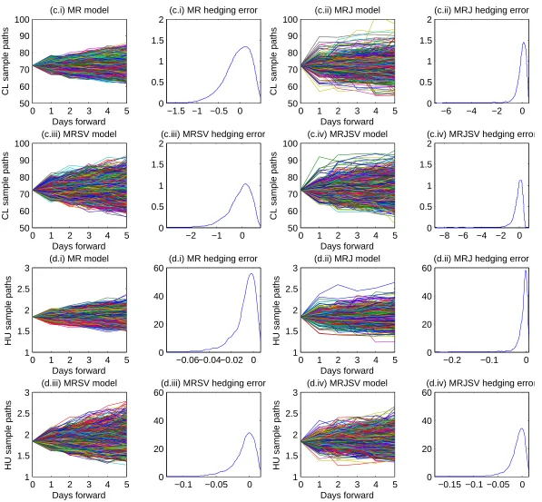
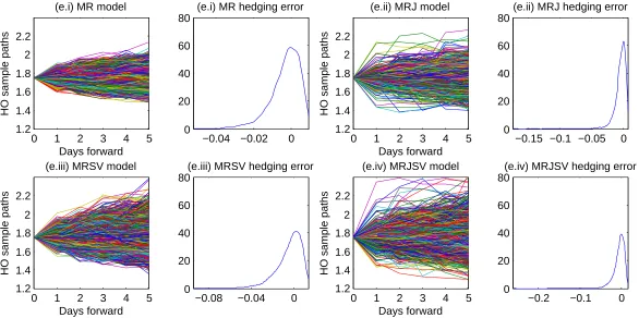
Fig. 1: Simulated commodity price paths and hedging error distributions
Simulated (deseasonalized) price paths of each underlying commodity (panel a: CB $/bbl, panel b: GO -$/mt, panel c: CL - $/bbl, panel d: HU - $/gal, panel e: HO - $/gal) across a 5-day hedge period coupled with the distributions (Matlab’s kernel smoothing function estimates) of the hedging errors at the closing of a week-long dynamic delta strategy with daily rebalancing without model misspecification, under the four data-generating processes (i: MR, ii: MRJ, iii: MRSV, iv: MRJSV). Hedging error is defined as the difference between the value of the daily-rebalanced hedge portfolio and the value of a 1-month to maturity, daily-averaged ATM arithmetic Asian option for the 1-week hedge period.
0 1 2 3 4 5
50 60 70 80 90
(a.i) MR model
Days forward
CB sample paths
−2 −1 0
0 0.5 1 1.5 2
(a.i) MR hedging error
0 1 2 3 4 5
50 60 70 80 90
(a.ii) MRJ model
Days forward
CB sample paths
−4 −2 0
0 0.5 1 1.5 2
(a.ii) MRJ hedging error
0 1 2 3 4 5
50 60 70 80 90
(a.iii) MRSV model
Days forward
CB sample paths
−3 −2 −1 0
0 0.5 1 1.5 2
(a.iii) MRSV hedging error
0 1 2 3 4 5
50 60 70 80 90
(a.iv) MRJSV model
Days forward
CB sample paths
−6 −4 −2 0
0 0.5 1 1.5 2
(a.iv) MRJSV hedging error
0 1 2 3 4 5
400 500 600 700
(b.i) MR model
Days forward
GO sample paths
−15 −10 −5 0
0 0.1 0.2 0.3
(b.i) MR hedging error
0 1 2 3 4 5
400 500 600 700
(b.ii) MRJ model
Days forward
GO sample paths
−40 −20 0
0 0.1 0.2 0.3
(b.ii) MRJ hedging error
500 600 700
(b.iii) MRSV model
GO sample paths
0.1 0.2 0.3
(b.iii) MRSV hedging error
500 600 700
(b.iv) MRJSV model
GO sample paths
0.1 0.2 0.3