City, University of London Institutional Repository
Citation:
Fring, A., Dey, S. & Gouba, L. (2015). Milne quantization for non-Hermitian systems. Journal of Physics A: Mathematical and Theoretical, 48, p. 40. doi: 10.1088/1751-8113/48/40/40FT01This is the accepted version of the paper.
This version of the publication may differ from the final published
version.
Permanent repository link:
http://openaccess.city.ac.uk/12484/Link to published version:
http://dx.doi.org/10.1088/1751-8113/48/40/40FT01Copyright and reuse: City Research Online aims to make research
outputs of City, University of London available to a wider audience.
Copyright and Moral Rights remain with the author(s) and/or copyright
holders. URLs from City Research Online may be freely distributed and
linked to.
City Research Online: http://openaccess.city.ac.uk/ [email protected]
arXiv:1507.03809v1 [quant-ph] 14 Jul 2015
Milne quantization for non-Hermitian systems
Sanjib Dey1,2, Andreas Fring3 and Laure Gouba4
1 Centre de Recherches Math´ematiques (CRM), Universit´e de Montr´eal, Montr´eal - H3C 3J7, Qu´ebec, Canada
2 Department of Mathematics and Statistics, Concordia University, Montr´eal - H3G 1M8, Qu´ebec, Canada
3 Department of Mathematics, City University London, London EC1V 0HB, UK 4 The Abdus Salam International Centre for Theoretical Physics (ICTP),
Strada Costiera 11, I-34151 Trieste Italy
E-mail: [email protected],[email protected],[email protected]
Abstract: We generalize the Milne quantization condition to non-Hermitian systems.
In the general case the underlying nonlinear Ermakov-Milne-Pinney equation needs to be replaced by a nonlinear integral differential equation. However, when the system is PT-symmetric or/and quasi/pseudo-Hermitian the equations simplify and one may employ the original energy integral to determine its quantization. We illustrate the working of the general framework with the Swanson model and two explicit examples for pairs of supersymmetric Hamiltonians. In one case both partner Hamiltonians are Hermitian and in the other a Hermitian Hamiltonian is paired by a Darboux transformation to a non-Hermitian one.
1. Introduction
We analyze two types of non-Hermitian systems, in one case we exploit the fact that the model is quasi/pseudo-Hermitian, the Swanson model, and in the other that it is
PT-symmetric, a supersymmetric pair in which one of the partner Hamiltonians is non-Hermitian.
Our manuscript is organized as follows: In section 2 we recall the key features of the Milne quantization procedure and generalize it to a general non-Hermitian setting. In section 3 we discuss the Swanson model and in section 4 we provide two explicit examples for pairs of supersymmetric Hamiltonians, where in one case both partner Hamiltonians are Hermitian and in the other only one of them. Our conclusions and outlook are stated in section 5.
2. The Milne quantization for Hermitian and non-Hermitian systems
We commence by briefly recalling the key idea of the solution procedure and quantization method proposed originally by Milne in 1930 [1]. Its starting point is the time-independent Schr¨odinger equation in the form
ψ′′(x) +k2(x)ψ(x) = 0, (2.1)
where the continuous energy parameter E and the potential V(x) are combined into the local wavevector k2(x) =~2/2m[E−V(x)]. Assuming the solution to equation (2.1) to be
of the general form
ψ(x) =N ρ(x) sin [φ(x) +α], (2.2) with normalization constantN, constant phaseα, amplitudeρ(x) and variable phaseφ(x) a direct substitution leads to the constraining equations
ρ′′(x) +k2(x)ρ(x) = λ
2
ρ3(x), and ρ
2(x)φ′(x) =λ, (2.3)
withλbeing some arbitrary constant. The first equation in (2.3) is known as the Ermakov-Milne-Pinney (EMP) equation [2, 1, 3]. From (2.2) it is clear that its solution together with a solution for the auxiliary equation for the phase function will lead to an exact solution for the time-independent Schr¨odinger equation (2.1) for generic values of E. Notice that when we neglect ρ′′(x), the two equations in (2.3) combine intoφ′(x) =k(x) which corresponds
to the WKB approximation. In what follows we will employ Pinney’s [3] general solution for the EMP-equation1
ρ(x) =
s
ψ21(x) + λ
2
W2ψ 2
2(x), (2.4)
with ρ(x0) = ρ0 6= 0, ρ′(x0) = ρ′0, −∞ < x0 <∞. Here ψ1, ψ2 are the two fundamental
solutions of the Schr¨odinger equation (2.1) and W :=W(ψ1, ψ2) = ψ1ψ′2−ψ′1ψ2 denotes the corresponding Wronskian. Integrating the second equation in (2.3) directly and taking
1
the initial conditions to beψ1(x0) = 1,ψ2(x0) = 0,ψ′1(x0) = 1,ψ′2(x0) =λimpliesW =λ
and leads to the general solution of equation (2.1) expressed in terms of the solutions to the EMP-equation
ψ(x) =N ρ(x) sin
W
Z x
x0
ρ−2(s)ds+α
. (2.5)
Next we implement the boundary conditions. Demanding the wavefunctionψ(x) to vanish at the boundaries then implies the quantization condition
I(E) = W(E)
π
Z ∞
−∞
ρ−2(s, E)ds=n∈N, (2.6)
when ρ(x) is non-vanishing, meaning that any solution En to I(En) = n constitutes a
bound state energy. Note that the value of I(E) is not sensitive to the normalization factors in the fundamental solution.
When the potential and possibly also the energy eigenvalues are complex the general treatment is more involved. In that case we can make the Ansatz
ψ(x) =N ρ(x)eiφ(x), (2.7) withρ(x), φ(x)∈Rand separate the wavevector into its real and imaginary partk2 =κ+iτ.
The substitution of (2.7) into the time-independent Schr¨odinger equation then yields the two constraining equations when reading off the real and imaginary parts
ρ′′(x) +κ(x)ρ(x) =ρ(x)φ′(x), and φ′′(x)ρ(x) + 2φ′(x)ρ′(x) +τ(x)ρ(x) = 0. (2.8) Combining these two equations generalizes the EMP-equation (2.3) to
ρ′′(x) +κ(x)ρ(x) = 1
ρ3(x)
λ−
Z x
τ(s)ρ2(s)ds
2
(2.9)
with
φ(x) =λ
Z x
ρ−2(s)ds−
Z x
ρ−2(t)
Z t
τ(s)ρ2(s)ds
dt. (2.10)
Evidently when τ = 0 we recover (2.3). These equations are difficult to solve, even in an approximate fashion. However, we may assume that the quantization condition (2.6) still holds whenW(E)∈Rand Im[ρ2(s, E)] is an odd function ins. We will demonstrate below
that these properties can be attributed to thePT-symmetry of the models.
3. A quasi-Hermitian model, the Swanson Hamiltonian
Quasi/pseudo-Hermitian Hamiltonian systems constitute a large subclass of non-Hermitian systems [6, 7, 8]. They are characterized by the fact that their non-Hermitian Hamiltonian
H can be mapped to an isospectral Hermitian counterpart h by means of a similarity transformation h = ηHη−1. The map η is sometimes referred to as the Dyson map [9] and satisfies certain properties. A prime example for which this map and all other relevant quantities are known in its explicit analytic form is the Swanson model [10]
HS =ω
witha=p
ω/2x+i/√2ωp,a†=p
ω/2x−i/√2ωp. Evidently HS is only Hermitian when
α=β, but its isospectral Hermitian counterpart is known to be [11]
hS =
µ+
2 p
2+ µ−
2 x
2, (3.2)
with
µ±= −λ(α+β) +ω∓(α+β−λω)
q
1− (1−(α+λ2β)(−αλω−β)2)2
(1±λ)ω±1 , λ∈[−1,1]. (3.3)
The eigenvalue spectrum for both Hamiltonians is
En=
n+1
2
p
ω2−4αβ, n∈N, (3.4)
and thus real for ω2 ≥4αβ. The corresponding time-independent Schr¨odinger equations are exactly solvable for both Hamiltonians. The two fundamental solutions for the one corresponding to hS can be expressed in terms of parabolic cylinder functions, but in the
current context it is more convenient to employ the solutions in terms of the closely related Whittaker functions
ψ1(x) = √1
xM2√µE −µ+
,−41
rµ
−
µ+x
2
Θ(x) + √i
xM2√µE −µ+
,−14
rµ
−
µ+x
2
Θ(−x), (3.5)
ψ2(x) = √1
xW2√µE −µ+
,−14
rµ
−
µ+x
2
Θ(x) +√i
xW2√µE −µ+
,−14
rµ
−
µ+x
2
Θ(−x). (3.6)
We neglect here normalization factors for the above mentioned reason. Unlike the solutions in terms of parabolic cylinder functions this choice guarantees thatψ1,2(x)∈Rorψ1,2(x)∈
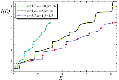
iR, such that ρ(x), W(E) ∈ R. Using these expressions we compute the energy integral
I(E) in (2.6) and depict our results in figure 1.
The energy eigenvalues are located precisely at the expected values at points of inflec-tion of the funcinflec-tion I(E).
4. Non-Hermitian models with supersymmetric Hermitian counterparts
Now we study a model in which we exploit thePT-symmetry of the system. We consider a pair of supersymmetric quantum mechanical [12, 13, 14, 15] models described by the two Hamiltonians
H±=L±L∓ =−
d2 dx2 +U
2(x)
±U′(x) =− d 2
dx2 +V±(x), (4.1)
involving the so-called superpotential U(x). It is easily verified that the solutions to the time-independent Schr¨odinger equationsH±ψ±=Eψ±are related to each other by means
of the two intertwining operatorsL±
L±:=±
d
dx+U(x), ψ±=
1
√
0 2 4 6 8 0
2 4 6 8 10
12 =1/2, , =1/4
=1, , =1/4
=3/2, =1, =1/3 I(E)
[image:6.612.97.491.87.352.2]E
Figure 1: Energy integralsI(E) for the Swanson model, withI((2n−1)/4√2) =I(En−1) =n∈N
forω = 1/2,α= 1/8,β = 1/4 I((2n−1)/2√2) =I(En−1) =n∈Nforω = 1,α= 1/2,β = 1/4
andI((2n−1)11/4√2) =I(En−1) =n∈Nforω= 3/2,α= 1,β= 1/3
Denoting now the two fundamental solutions to the Schr¨odinger equation by ψ and χ, Ioffe and Korsch [16] found that the corresponding Wronskians and solutions to the EMP-equations
W±:=W ψ±, χ±
, ρ±=
q
ψ2±+χ2
± (4.3)
are related to each other as
W+=W−, and Eρ2±= L±ρ∓
2
+W∓
ρ2 ∓
. (4.4)
The first identity follows from a direct substitution of the wavefunction in (4.2) into the defining relation for the Wronskian, the use of the Schr¨odinger equation and recalling that
dW/dx = 0. The derivation of the second identity follows from a direct evaluation. We also add here for later use an intermediate relation from that computation
Eρ2+=U2ρ2−+U(ρ2−)′+ ψ′−2
+ χ′−2
. (4.5)
this case. Separating the real and imaginary parts in the superpotentials in the form
U(x) =a(x) +ib(x), with a(x), b(x)∈R,a(x) = 1
2
d
dxlnb(x), (4.6)
they observed that one obtains a real and a complex partner potential
V−(x) =
3b′2
4b(x)2 −
b′′(x)
2b(x) −b(x)
2 ∈R, (4.7)
V+(x) =
b′′(x)
2b(x) −
b′2
4b(x)2 −b(x)
2+ 2ib′(x) /
∈R. (4.8)
In the following it will be important to utilize the effect of the parity operatorP and time-reversal operatorT on the various quantities involved. Our main requirement is that
V+ becomesPT-symmetric, which is achieved as follows
PT :a(x)→ −a(x), b(x)→b(x); PT :U(x)→ −U(x), V±(x)→V±(x). (4.9)
In order to obtain real eigenvaluesE ∈R, usually referred to as the spontaneously unbroken
PT-symmetric regime, we also require the wavefunctions to be symmetric with regard to the anti-linear PT-operator [18, 19]
PT :ψ±(x),→ψ±(x), χ±(x)→χ±(x), W±(x)→ −W±(x), ρ±(x)→ρ±(x). (4.10)
When assuming thatψ−, χ−∈R, it follows from (4.5) and the subsequent use of the second
relation in (4.4) that
Im Eρ2+
= Imh L+ρ−
2i
= d
dx bρ
2 −
. (4.11)
This implies that for real energies there will not be any contribution to the integral in (2.6) from the imaginary part of the integrand 1/ρ2+ as it will be an odd function. The assumptionψ−, χ−∈Ralso guarantees thatW−∈Rand therefore by the first relation in
(4.4) W+∈R, which are the requirements mentioned at the end of section 2. 4.1 A Hermitian/Hermitian supersymmetric pair
As an illustration for the working of the conventional Milne quantization for supersym-metric pairs we first consider a well studied exactly solvable in the mathematical physics literature, [20, 21, 22], the P¨oschl-Teller model [23]. Taking the superpotential to be of the form
U(x) =λtanx−κcotx, κ, λ∈R,0≤x≤π/2. (4.12)
equation (4.1) yields the pair of potentials
V±(x) =λ(λ±1) sec2x+κ(κ±1) csc2x−(λ+κ)2, (4.13)
withV−(x) being the standard P¨oschl-Teller potential. The fundamental solutions are well
known. We have
ψ−1(x) = sinκxcosλx2F1
"
κ+λ−E˜
2 ,
κ+λ+ ˜E
2 ;κ+
1 2; sin
2x
#
, (4.14)
ψ−2(x) = sin1−κxcosλx2F1
"
1−κ+λ−E˜
2 ,
1−κ+λ+ ˜E
2 ;
3
2−κ; sin
2x
#
and
ψ+1(x) = sinκ+1xcosλ+1x2F1
"
2 +κ+λ−E˜
2 ,
2 +κ+λ+ ˜E
2 ;κ+
3 2; sin
2x
#
,(4.16)
ψ+2(x) = sin−κxcosλ+1x2F1
"
1−κ+λ−E˜
2 ,
1−κ+λ+ ˜E
2 ;
1
2 −κ; sin
2x
#
, (4.17)
where 2F1 denoted hypergeometric function and we abbreviated ˜E :=
p
(κ+λ)2+E.
Solutions to the EMP-equation are simply obtained from (2.4)
ρ±(x) =
q
ψ±1(x)2
+
ψ±2(x)2
, (4.18)
which allows us to compute the energy integrals (2.6) to
I±(E) =
W±(E)
π
Z π/2
0
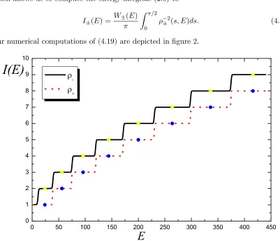
ρ−2± (s, E)ds. (4.19)
Our numerical computations of (4.19) are depicted in figure 2.
0 50 100 150 200 250 300 350 400 450 0
1 2 3 4 5 6 7 8 9 10
-+ I(E)
[image:8.612.96.497.266.612.2]E
Figure 2:Energy integralsI±(E) for a supersymmetric pair of P¨oschl-Teller potentials for coupling constants κ = 2, λ = 3, with I−(0) = I+(24) = 1, I−(24) = I+(56) = 2, I−(56) = I+(96) = 3,
I−(96) =I+(144) = 4, I−(144) = I+(200) = 5, I−(200) = I+(264) = 6, I−(264) = I+(336) = 7,
I−(336) =I+(416) = 8 andI−(416) = 9.
For the selected values of the coupling constantk= 2,λ= 3 the solutions toI±(E±n) =
n+ 1 yield E0− = 0, E+
the well known quantization condition obtained from demanding that limx→0ψ±1(x) =
limx→π/2ψ±1(x) = 0, achieved by setting the first entry of the hypergeometric function2F1
to −nwithn= 0,1,2, . . .
4.2 A Hermitian/Non-Hermitian supersymmetric pair
Next we consider a superpotential giving rise to a Hermitian potential paired with a non-Hermitian potential as proposed in [17]. We take the superpotential U(x) to be of the form
U(x) =−1
2tanhx+
i
2(1−2λ) sechx, λ∈R, (4.20) such that the real and imaginary parts are related as in (4.6). As expected, when evaluating (4.1) one of the partner potentials turn out to be real
V−(x) =
1
4+ (λ−λ
2) sech2x, (4.21)
whereas the other one becomes complex
V+(x) =
1
4 − 1−λ+λ
2
sech2x+i(2λ−1) sechxtanhx, (4.22) albeit PT-symmetric. The fundamental solutions are in this case
ψ−1(x) = sinhxcoshλx2F1
µ−, µ+;
3
2;−sinh
2x
, (4.23)
ψ−2(x) = coshλx2F1
µ−−1
2, µ+− 1 2;
1
2;−sinh
2x
, (4.24)
and according to (4.2) we obtain the solutions for the partner Hamiltonian as
ψ+1(x) = cosh
λ−1(x)
12√E
6
2 cosh2x+ (2λ−1) sinhx(sinhx−i)
2F1
µ−, µ+;
3
2;−sinh
2x
− 1
4sinh
2(2x) [4E+ 4λ(λ+ 2) + 3] 2F1
µ−+ 1, µ++ 1;5
2;−sinh
2x
, (4.25)
ψ+2(x) = cosh
λ−1(x)
4√E
2(2λ−1)(sinhx−i)2F1
µ−−1
2, µ+− 1 2;
1
2;−sinh
2x
+ 1−4E−4λ2
sinhxcosh2x2F1
µ−+
1 2, µ++
1 2;
3
2;−sinh
2x
, (4.26)
whereµ±:= (2 + 2λ±√1−4E)/4.
We have now all the ingredients to evaluate the energy integrals in (4.19). Our results are depicted in figure 3.
For the selected values of the coupling constantλthe solutions toI±(En±) =n+1 yield
E0−=−42,E+
n =En−+1 =−(n−6)(n−7) forn= 0,1,2, . . . This is again the quantization
condition obtained from demanding that limx→±∞ψ±1(x) = 0, achieved by setting the first
entry of the hypergeometric function2F1 to−nwithn= 0,1,2, . . .The remarkable feature
-45 -40 -35 -30 -25 -20 -15 -10 -5 0 0
1 2 3 4 5 6 7 8
-+ I(E)
[image:10.612.100.491.84.356.2]E
Figure 3: Energy integralsI±(E) for a supersymmetric pair potentialsV±in (4.21), (4.22) for the coupling constant λ= 15/2, with I−(−42) = I+(−30) = 1, I−(−30) =I+(−20) = 2, I−(−20) =
I+(−12) = 3,I−(−12) =I+(−6) = 4,I−(−6) =I+(−2) = 5,I−(−2) =I+(0) = 6, andI−(0) = 7.
5. Conclusion
We demonstrated that the Milne quantization procedure can be successfully adopted to non-Hermitian systems that are either quasi/pseudo-Hermitian orPT-symmetric. For each scenario we provided an explicit example. We proposed some generalized formulae for the generic non-Hermitian case, which are left as a challenge to be solved for some concrete example.
Building on the success, it is to be expected that this method can be applied also to systems for which the quantization is still incompletely understood [24], such as the complex Mathieu system currently of great interest as it corresponds to the eigenvalue equation of the collision operator in a two-dimensional Lorentz gas.
Acknowledgements: SD is supported by the Postdoctoral Fellowship jointly funded by the Laboratory of Mathematical Physics of the Centre de Recherches Math´ematiques (CRM) and by Prof. Syed Twareque Ali, Prof. Marco Bertola and Prof. V´eronique Hussin. LG is supported by the Abdus Salam International Centre for Theoretical Physics (ICTP).
References
[2] V. Ermakov, Transformation of differential equations,, Univ. Izv. Kiev.20, 1–19 (1880).
[3] E. Pinney, The nonlinear differential equation y′′
+p(x)y+c/y3= 0, Proc. Amer. Math.
Soc.1, 681(1) (1950).
[4] C. M. Bender and H. F. Jones, WKB analysis of PT-symmetric Sturm–Liouville problems, J. Phys. A 45, 444004 (2012).
[5] C. Eliezer and A. Gray, A note on the time-dependent harmonic oscillator, SIAM J. on Appl. Math. 30, 463–468 (1976).
[6] J. Dieudonn´e, Quasi-hermitian operators, Proceedings of the International Symposium on Linear Spaces, Jerusalem 1960, Pergamon, Oxford , 115–122 (1961).
[7] F. G. Scholtz, H. B. Geyer, and F. Hahne, Quasi-Hermitian Operators in Quantum Mechanics and the Variational Principle, Ann. Phys.213, 74–101 (1992).
[8] A. Mostafazadeh, Pseudo-Hermitian Representation of Quantum Mechanics, Int. J. Geom. Meth. Mod. Phys.7, 1191–1306 (2010).
[9] F. J. Dyson, Thermodynamic Behavior of an Ideal Ferromagnet, Phys. Rev. 102, 1230–1244 (1956).
[10] M. S. Swanson, Transition elements for a non-Hermitian quadratic Hamiltonian, J. Math. Phys.45, 585–601 (2004).
[11] D. P. Musumbu, H. B. Geyer, and W. D. Heiss, Choice of a metric for the non-Hermitian oscillator, J. Phys. A40, F75–F80 (2007).
[12] E. Witten, Dynamical breaking of supersymmetry, Nucl. Phys. B188, 513 (1981).
[13] F. Cooper and B. Freedman, Aspects of Supersymmetric Quantum Mechanics, Annals Phys.
146, 262 (1983).
[14] E. Witten, Constraints on supersymmetry breaking, Nucl. Phys. B202, 253 (1982).
[15] F. Cooper, A. Khare, and U. Sukhatme, Supersymmetry and quantum mechanics, Phys. Rept.251, 267–385 (1995).
[16] M. V. Ioffe and H. Korsch, Nonlinear supersymmetric (Darboux) covariance of the Ermakov-Milne-Pinney equation, Phys. Lett. A 311, 200–205 (2003).
[17] B. Bagchi and R. Roychoudhury, A New PT symmetric complex Hamiltonian with a real spectrum, J.Phys.A33, L1–L3 (2000).
[18] E. Wigner, Normal form of antiunitary operators, J. Math. Phys.1, 409–413 (1960).
[19] C. M. Bender and S. Boettcher, Real Spectra in Non-Hermitian Hamiltonians Having PT Symmetry, Phys. Rev. Lett. 80, 5243–5246 (1998).
[20] H. Kleinert and I. Mustapic, Summing the spectral representations of P¨oschl–Teller and Rosen-Morse fixed-energy amplitudes, J. Math. Phys. 33, 643(20) (1992).
[21] J.-P. Antoine, J.-P. Gazeau, P. Monceau, J. R. Klauder, and K. A. Penson, Temporally stable coherent states for infinite well and P¨oschl–Teller potentials, J. Math. Phys.42, 2349–2387 (2001).
[23] G. P¨oschl and E. Teller, Bemerkungen zur Quantenmechanik des anharmonischen Oszillators, Z. Phys. 83, 143–151 (1933).