Lattice and string worldsheet in AdS/CFT: a numerical study

City, University of London Institutional Repository

Citation

: Forini, V., Bianchi, L., Bianchi, M. S., Leder, B. & Vescovi, E. (2015). Lattice and

This is the published version of the paper.

This version of the publication may differ from the final published

version.

Permanent repository link:

Link to published version

:

Copyright and reuse:

City Research Online aims to make research

outputs of City, University of London available to a wider audience.

Copyright and Moral Rights remain with the author(s) and/or copyright

holders. URLs from City Research Online may be freely distributed and

linked to.

Lattice and string worldsheet in AdS/CFT:

a numerical study

Valentina Forini∗

Humboldt-Universität zu Berlin, Zum Großen Windkanal 6, 12489 Berlin, Germany

E-mail:[email protected]

Lorenzo Bianchi

Humboldt-Universität zu Berlin, Zum Großen Windkanal 6, 12489 Berlin, Germany II. Institut für Theoretische Physik, Universität Hamburg, Luruper Chaussee 149, 22761 Hamburg, Germany

E-mail:[email protected]

Marco S. Bianchi

Center for Research in String Theory - School of Physics and Astronomy Queen Mary University of London, Mile End Road, London E1 4NS, UK E-mail:[email protected]

Bjoern Leder

Institutsrechenzentrum, Institut für Physik

Humboldt-Universität zu Berlin, Newtonstr. 15, 12489 Berlin, German E-mail:[email protected]

Edoardo Vescovi

Humboldt-Universität zu Berlin, Zum Großen Windkanal 6, 12489 Berlin, Germany E-mail:[email protected]

We consider a possible discretization for the gauge-fixed Green-Schwarz (two-dimensional) sigma-model action for the Type IIB superstring and use it for measuring the cusp anomalous

dimension of planarN =4 SYM as derived from string theory. We perform lattice simulations

employing a Rational Hybrid Monte Carlo (RHMC) algorithm and a Wilson-like fermion dis-cretization. In this preliminary study, we compare our results with the expected behavior for very

large values ofg= √λ

4π, which is the perturbative regime of the sigma-model, and find a

qual-itative agreement at finite lattice spacing. For smallergthe continuum limit is obstructed by a

divergence. We also detect a phase in the fermion determinant, whose origin we explain, which

for smallgleads to a sign problem not treatable via standard reweigthing. Results presented here

are discussed thoroughly in [1].

The 33rd International Symposium on Lattice Field Theory 14 -18 July 2015

Kobe International Conference Center, Kobe, Japan*

∗_Speaker.

Lattice and string worldsheet in AdS/CFT: a numerical study Valentina Forini

1. Discussion

An impressive amount of evidence obtained in the last decade indicates the maximally super-symmetric and superconformalN =4 planar super Yang-Mills (SYM) theory as the first example of a non-trivially interacting, four-dimensional gauge theory that might be exactly solvable. The “evidence” refers to the several results, obtained relying on the assumption of an all-order quantum integrability for this model [2], that have been confirmed by direct perturbative computations both in gauge theory and in what AdS/CFT assigns as string dual toN =4 SYM - the Type IIB, Green-Schwarz string propagating in the maximally supersymmetric backgroundAdS_5×S5supported by a self-dual Ramond-Ramond (RR) five-form flux. However, without the assumption of quantum integrability, very little is known about the theory at finite coupling. Here a lattice approach may be powerful. A rich and interesting program of puttingN =4 SYM on the lattice is being carried out for some years by Catterall et al. [3]1.

Following the earlier proposal of [5], we take a different lattice-based route to investigate the finite coupling region of the N =4 SYM theory, discretizing the dual two-dimensional string worldsheet. We focus on a particularly important observable of the theory – the cusp anomalous dimension – which we describe in Section2. From the dual point of view provided by the AdS/CFT correspondence [6], this quantity is measured by the path integral of an open string bounded by a cusped Wilson loop at the AdS boundary, which is where the four-dimensional gauge-theory lives in the holographic picture. This string worldsheet is a highly non-trivial 2d non-linear sigma-model with rich non-perturbative dynamics.

We propose a discretization of such a model in Section 3. It is important to emphasize that,

since the gauge symmetries of the model (bosonic diffeomorphisms andκ-symmetry) are all fixed,

this isnota definition of the Green-Schwarz worldsheet string model à la Wilson lattice-QCD, but

rather an investigation of possible routes via which lattice simulations could be an efficient tool in numerical holography.

In Section4we describe our lattice simulations, which use the Rational Hybrid Monte Carlo

(RHMC) algorithm. Our line of constant physics demands physical masses to be kept constant while approaching the continuum limit, which in the case of finite mass renormalization requires

no tuning of the “bare” mass parameter of the theory (the light-cone momentumP+). For one of

the bosonic fields entering the Lagrangian we determine the correlator and physical mass, confirm-ing the expected finite renormalization and thus no need of tunconfirm-ing. A good agreement with the perturbative sigma-model expectation is reached for both the correlators and the observable under

investigation at very large values of the couplingg=√λ/(4π)(λ is the ’t Hooft coupling of the

AdS/CFT dual gauge theory) 2. For smaller g we observe a divergence, possibly signaling the

presence of infinite mass renormalization for the field content of the theory which so far we have not analyzed and whose study we leave for the future.

One important result of our analysis is the detection of a phase in the fermionic determinant, re-sulting from integrating out the fermions. This phase is introduced by the linearization of fermionic interactions used in [5]. For values of the coupling approaching the non-perturbative regime

(cor-responding to weakly-coupledN =4 SYM) the phase undergoes strong fluctuations, signaling a

severe sign problem. It would be desirable to find alternative ways to linearize quartic fermionic interactions, with resulting Yukawa terms leading to a real, positive definite fermionic determinant. Attempts in this direction are ongoing and we hope to report on them in the near future.

2. The observable: cusp anomaly of planarN =4SYM from string theory

The cusp anomaly of N =4 SYM, in this framework often simply referred to as “scaling

1_{We refer the reader to the POS contribution [4] for a report on interesting recent results.} 2_{In the AdS/CFT context, where the ’t Hooft coupling}

λ ∼g2 is used as relevant parameter, the largegregion is naturally referred to as “strong coupling” regime. The string worldsheet sigma-model of interest here, for which perturbation theory is a 1/gexpansion, is however weakly-coupled at largeg.

function”3, is a function of the coupling and it governs the renormalization of a Wilson loop with a light-like cusp inN =4 super Yang-Mills, as well as the leading behavior, in the large spin S

regime, of the anomalous dimension of twist-two operators. According to AdS/CFT, any Wilson loop expectation value should be represented by the path integral of an open string ending at the AdS boundary

hW[C_cusp]_{i ≡}Z_cusp=

Z

[DδX][DδΨ]e−Scusp[Xcl+δX,δΨ]_=e−Γeff_≡e−18f(g)V2 . (2.2)

Above,Xcl=Xcl(t,s)- witht,sthe temporal and spatial coordinate spanning the string worldsheet

- is the classical solution of the string equations of motion describing the world surface of an open string ending on a null cusp [8]. S_cusp[X+δX,δΨ]is the action for field fluctuations over it – the

fields being both bosonic and fermionic string coordinatesX(t,s), Ψ(t,s)– and is reported below in equation (2.4) in terms of the effective bosonic and fermionic degrees of freedom remaining af-ter gauge-fixing. Since the fluctuation Lagrangian has constant coefficients, the worldsheet volume

V2=

R

dtdssimply factorizes out4in front of the function of the coupling f(g), as in the last

equiv-alence in (2.2). The scaling function can be evaluated perturbatively in gauge theory (g1), and

in sigma-model loop expansion (g1) as in (2.5) below. Assuming all-order integrability of the

spectral problem for the relevant operators and taking a thermodynamical limit of the

correspond-ing asymptotic Bethe Ansatz, an integral equation [9] can be derived which gives f(g)exactly at

each value of the coupling.

Rather than partition functions, in a lattice approach it is natural to study vacuum expectation values. In simulating the vacuum expectation value of the “cusp” action

hScuspi =

R

[DδX][DδΨ]Scuspe−Scusp

R

[DδX][DδΨ]e−Scusp =−g

dlnZ_cusp dg ≡g

V2

8 f

0_{(g), (2.3)}

we are therefore supposed to obtain information on thederivativeof the scaling function5. In the continuum, the AdS5×S5 superstring action Scusp describing quantum fluctuations

around the null-cusp background can be written after Wick-rotation as [8]

Scusp=g

Z

dtds

n

|∂tx+1₂x|2+_z14|∂sx−

1 2x|2+

∂tzM+1₂zM+_zi2zNηi ρ

MNi

jη

j2

+1

z4 ∂sz

M −1

2z

M2

+i θi∂tθi+ηi∂tηi+θi∂tθi+ηi∂tηi

− 1

z2 η

i ηi

2

(2.4)

+2i

h

1

z3zMηi ρM

i j ∂sθ

j₋1

2θ

j₋i

zη

j

∂sx−1₂x

+1

z3zMηi(ρM†)i j

∂sθj−1₂θj+i_zηj ∂sx−1₂x

∗ i o

Above, x,x∗ are the two bosonicAdS5 (coordinate) fields transverse to theAdS3 subspace of the

classical solution, andzM(M=1,···,6)are the bosonic coordinates of theAdS5×S5background in

Poincaré parametrization, withz=pzMzM, remaining after fixing a “AdS light-cone gauge” [10]. 3_{The “scaling function” f(g)is in fact the coefficient of logSin the large spinSanomalous dimension}

∆of leading twist operators∆= f(g)logS+O(logS/S). It equals twice the cusp anomalous dimensionΓcuspof light-like Wilson

loops [7]

hW[Ccusp]_{i ∼}e−ΓcuspγlnΛUV

ΛIR , (2.1)

whereγis the large, real parameter related to the geometric angleφof the cusped Wilson loop byiγ=φ. The expectation value above is in fact extracted in the large imaginaryφlimit.

4_{As mentioned above, f(g)equals twice the coefficient of the logarithmic divergence in (2.1), for which the stringy} counterpart should be the infinite two-dimensional worldsheet volume. The further normalization ofV2with a 1/4 factor

follows the convention of [8].

5_{Here our analysis is different from the one in [5]. In particular,hSi ∼} f(g)

Lattice and string worldsheet in AdS/CFT: a numerical study Valentina Forini

The fieldsθi,ηi,i=1,2,3,4 are 4+4 complex anticommuting variables for whichθi= (θi)†,ηi=

(ηi)†. They transform in the fundamental representation of theSU(4)R-symmetry and do not carry

(Lorentz) spinor indices. The matricesρi jMare the off-diagonal blocks ofSO(6)Dirac matricesγM

in the chiral representation and(ρMN)_ij = (ρ[Mρ†N])_ij are theSO(6)generators. The action (2.4)

is manifestly missing a massive parameter6, which we restore in the following defining it asm. We

emphasize that, in (2.4), local bosonic (diffeomorphism) and fermionic (κ-) symmetries originally

present have been fixed. With this action one can directly proceed to the perturbative evaluation of

the effective action in (2.2), up to two loops in sigma-model perturbation theory [8], obtaining for

the cusp anomaly (Kis the Catalan constant)

f(g) =4g

1₋3 log 2

4πg −

K

16π2g2+O(g

−3_{). (2.5)}

Furthermore, with the same action it is possible to study perturbatively the (non-relativistic) disper-sion relation for the field excitations over the classical string surface. For example, the corrections

to the masses of the bosonic fieldsx,x∗in (2.4) (defined as the values of energy at vanishing

mo-mentum) read [11]

m2_x(g) = m

2

2

1₋ 1

8g+O(g

−2_{), (2.6)}

where, as mentioned above, we restored the dimensionful parameterm. In what follows, we will

compute the lattice correlators of the fieldsx,x∗so to study whether our discretization changes the

renormalization pattern above.

3. Linearization and discretization

While the bosonic part of (2.4) can be easily discretized and simulated, Graßmann-odd fields

are formally integrated out, letting their determinant to become part – via exponentiation in terms

of pseudo-fermions, see (3.6) below – of the Boltzmann weight of each configuration in the

sta-tistical ensemble. In the case of higher-order fermionic interactions – as in (2.4), where they are

at most quartic – this is possible via the introduction of auxiliary fields realizing a linearization.

Following [5], one introduces 7 real auxiliary fields, one scalarφand aSO(6)vector fieldφM, with

a Hubbard-Stratonovich transformation

exp

n

−g Z

dtds

h

− 1 z2 η

i

ηi 2

+_zi2zNηiρ MN i

jηj 2i

} (3.1)

∼

Z

DφDφMexp n

−g

Z

dtds[1 2φ2+

√

2

z φ η2+

1

2(φM)2−i

√

2

z2 φMzN iηiρMN ijηj

]o.

Above, in the second line we have written the Lagrangian forφM so to emphasize that it has an

imaginary part, due to the fact that the bilinear form in round brackets is hermitian

iηiρMN ijηj †

=−i(ηj)†(ρMN ij)∗(ηi)†=−iηjρMNi

j

ηi=iηjρMN jiηi, (3.2)

as follows from the properties of theSO(6)generators (see for example Appendix A of [8]). Since the auxiliary vector fieldφMhas real support, the Yukawa-term for it setsa prioria phase problem, the only question being whether the latter is treatable via standard reweighing. Below we find evidence that this is not the case.

6_{As standard in the literature - the light-cone momentum can be consistently set to the unitary value,p}+_{=1. In the}

perspective adopted here, however, it is crucial to keep track of dimensionful parameters as they are in principle subject to renormalization.

After the transformation (3.1), the corresponding Lagrangian reads

L =_|∂tx+m₂x|2+_z14|∂sx−m₂x|2+(∂tzM+1₂zM)2+_z14(∂szM−m₂zM)2+1₂φ2+1₂(φM)2+ψTOFψ(3.3)

withψ≡(θi,θi,ηi,ηi)and

OF =



   

0 i∂t −iρM ∂s+m₂

_zM

z3 0

i∂t 0 0 −iρ_M† ∂s+m₂

_zM

z3

iz_zM3ρ M

∂s−m₂

0 2z_zM4ρ M

∂sx−mx₂

i∂t−AT

0 iz_zM3ρ

†

M ∂s−

m

2

i∂t+A −2z

M

z4ρ

†

M ∂sx∗−m

x

2∗



   

,(3.4)

A = √1

2z2φMρ

MN

zN−

1

√

2zφ +i zN

z2ρ

MN

∂tzM . (3.5)

The quadratic fermionic contribution resulting from linearization gives then formally a Pfaffian PfOF, which in order to enter the Boltzmann weight and thus be interpreted as a probability

-should be positive definite. For this reason, we proceed as in [5]

Z

DΨe−

R

dtdsΨTOFΨ_=PfO

F ≡(detOFO†F)

1 4 =

Z

DξDξ¯e− R

dtdsξ¯(OFO†F)−

1 4_ξ

, (3.6) where the second equivalence obviously ignores potential phases or anomalies and we are not being explicit in coupling-dependent Jacobians (see below).

The values of the discretised (scalar) fields are assigned to each lattice site, with periodic boundary conditions for all the fields except for antiperiodic temporal boundary conditions in the case of fermions. The discrete approximation of continuum derivatives are finite difference opera-tors defined on the lattice. A Wilson-like lattice operator must be introduced [1], such that fermion doublers are suppressed and the one-loop constant₋3 ln 2/π in (2.5) is recovered in lattice

pertur-bation theory. While such Wilson term explicitly breaks theSO(6)symmetry of the model, for the

SO(6)singlet quantities that we study – f(g)andx,x∗correlators – this might affect the way one

approaches the continuum limit, an issue which we address in the next Section.

The Monte Carlo evolution of the action (3.3) is generated by the standard Rational Hybrid

Monte Carlo (RHMC) algorithm, as in [5]. A detailed analysis of the precision of the fourth-root

approximation and the magnitude of the fermion matrix eigenvalues (3.4), error analysis and

auto-correlation times of the Monte Carlo histories is in [1].

4. Simulation, continuum limit and the phase

As discussed above, in the continuum model there are two parameters, the dimensionless

couplingg=√λ

4π and the mass scalem. In taking the continuum limit, the dimensionless physical

quantities that it is natural to keep constant are the physical masses of the field excitations rescaled

byL, the spatial lattice extent. This is our line of constant physics. For the example in (2.6), this

means

L2m2_x=const, which leads to L2m2_≡(NM)2_{=const, (4.1)}

where we defined the dimensionlessM=mawith the lattice spacinga. The second equation in

(4.1) relies first on the assumption thatgisnotrenormalized, which is suggested lattice perturbation

theory [1]. Second, one should investigate whether relation (2.6), and the analogue ones for the

other fields of the model, are still true in the discretized model -i.e. the physical masses undergo

only afiniterenormalization. In this case, at each fixedgfixingL2 m2 constant would be enough

to keep the rescaled physical masses constant, namely no tuning of the “bare” parametermwould

Lattice and string worldsheet in AdS/CFT: a numerical study Valentina Forini

0 0.2 0.4 0.6 0.8 1 1.2 1.4 0

0.2 0.4 0.6 0.8 1 1.2 1.4

tmx

(

m

eff x

)

2/m

2

L/a = 8, g=10 L/a = 10, g=10 L/a = 8, g=30 L/a = 10, g=30 L/a = 12, g=30

0 0.02 0.04 0.06 0.08 0.1 0.12 0

0.2 0.4 0.6 0.8 1 1.2

1/N

(

<

S

>

−

7

.

5

N

2)

/S

0

g= 100.00, Lm= 4 g= 30.00, Lm= 4 g= 10.00, Lm= 4

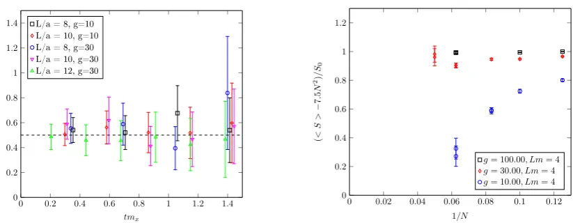
Figure 1: Left panel: Effective mass plot meff_x = 1

aln

Cx(t)

Cx(t+a), as calculated from the correlator

Cx(t) =∑s1,s2hx(t,s1)x ∗_(0,s

2)iof bosonic fieldsx,x∗in presence of Wilson terms.

Right panel:Plot of the ratio hSLATi−c N2/2

S0 , whereS0=M

2_N2_{g/2 andc/2=7.5(1).}

where indeed we find no (1/a) divergence for the ratiom2_x/m2– see the left panel in Figure1. In

the largegregion that we investigate the ratio considered approaches the expected continuum value

1/2. Having this as hint, and because with the proposed discretization we recover in perturbation

theory the one-loop cusp anomaly [1], we assume that in the discretized model no further scale but

the lattice spacingais present. Any observableFLATis therefore a functionFLAT=FLAT(g,N,M)of

the input (dimensionless) parametersg=√λ

4π,N=

L

aandM=a m. In Table1we list the parameters

of the simulations presented in this paper. At fixed couplinggand fixedm L_≡M N(large enough

so to keep finite volume effects∼e−m Lsmall), FLAT is evaluated for different values of N. The

continuum limit – which we do not attempt here – is then obtained extrapolating to infiniteN.

In measuring the action (2.3) on the lattice, we are supposed to recover the following general

behavior

hSLATi

N2 =

c

2+

1

8M

2_{g f}0_{(g), (4.2)}

where we have reinserted the parameterm, used thatV2=a2N2and added a constant contribution

in g which takes into account possible coupling-dependent Jacobians relating the (derivative of

the) partition function on the lattice to the one in the continuum. Measurements for the ratio

hSLATi−c N2/2 M2_N2_g/2 =

f0(g)

4 are, atg=100, in good agreement with

c

2 =7.5(1)– consistently with the

expectation [1] – and with the leading order prediction in (2.5) for which f0(g) =4. For lower

values ofg– red and blue curves in Figure1, right panel – we observe a deviation that obstructs

the continuum limit and is compatible with the presence of a divergence. This could be explained with the presence of infinite mass renormalization in those fields correlators which we have not considered so far, and whose investigation is left for the future.

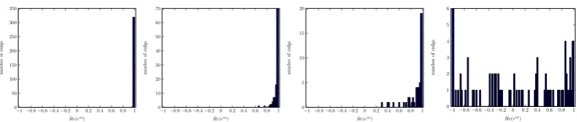
In proximity to g_∼1, severe fluctuations appear in the averaged phase of the Pfaffian – see

Figure2– signaling the sign problem mentioned in the Discussion.

Acknowledgments

We are particularly grateful to M. Bruno for initial collaboration, and to R. Roiban, D. Schaich, R. Sommer and A. Wipf for very useful elucidations. We also thank F. Di Renzo, H. Dorn, G. Eruzzi, M. Hanada and the theory group at Yukawa Institute, B. Hoare, B. Lucini, J. Plefka, A. Schwimmer, S. Theisen, P. Töpfer, A. Tseytlin and U. Wolff for useful discussions.

References

[1] L. Bianchi, M. S. Bianchi, V. Forini, B. Leder, E. Vescovi, to appear.

−1−0.8−0.6−0.4−0.2 0 0.20.4 0.60.8 1 0

50 100 150 200 250 300 350

Re(eiφ)

num

ber

of

cnfgs

−1−0.8−0.6−0.4−0.20 0.2 0.40.6 0.8 1 0

10 20 30 40 50 60 70

Re(eiφ)

num

ber

of

cnfgs

−1−0.8−0.6−0.4−0.2 0 0.2 0.4 0.60.8 1 0

5 10 15 20

Re(eiφ)

num

ber

of

cnfgs

−1−0.8−0.6−0.4−0.2 0 0.2 0.4 0.6 0.8 1 0

1 2 3 4 5 6

Re(eiφ₎

num

ber

of

cnfgs

Figure 2: Histograms for the frequency of the real part (the imaginary part vanishes by symmetry) of the reweighting phase factoreiθ _{of the Pfaffian PfO}

F =|(detOF)

1

2|eiθ, based on the ensembles

generated atg=30,10,5,1 (from left to right). Atg=1 the observed_heiθ_{iis consistent with zero,}

thus preventing the use of standard reweighting.

g T/a_×L/a am Lm statistics [MDU] τint

10 16×8 0.5 4 900 2

20_×10 0.4 4 900 3

24×12 0.33333 4 821, 900 5 32×16 0.25 4 316, 357 10

30 16_×8 0.5 4 800 1

20×10 0.4 4 800 2

24×12 0.33333 4 900 4 32_×16 0.25 4 625, 800 8 40×20 0.2 4 300, 300 60

100 16×8 0.5 4 900 1

20_×10 0.4 4 750 2

32×16 0.25 4 411, 415 5

Table 1: Parameters of the simulations. The temporal extentT is always twice the spatial extent

L, which helps studying the correlators. The size of the statistics after thermalization is given in terms of Molecular Dynanic Units (MDU) which equal an HMC trajectory of length one. In the case of multiple replica the statistics for each replica is given. The typical auto-correlation time of the correlators is given in the last column.

[2] N. Beisertet al., Lett. Math. Phys.99, 3 (2012)

[3] S. Catterall, D. B. Kaplan and M. Unsal, Phys. Rept.484, 71 (2009)

[4] D. Schaich,LATTICE 2015 (2015) 242, arXiv:1512.01137 [hep-lat]

[5] R. W. McKeown and R. Roiban, arXiv:1308.4875 [hep-th].

[6] J. M. Maldacena, Phys. Rev. Lett.80, 4859 (1998)

[7] G. P. Korchemsky and G. Marchesini, Nucl. Phys. B406, 225 (1993)

[8] S. Giombi, R. Ricci, R. Roiban, A. A. Tseytlin and C. Vergu, JHEP1003, 003 (2010)

[9] N. Beisert, B. Eden and M. Staudacher, J. Stat. Mech.0701, P01021 (2007)

[10] R. R. Metsaev and A. A. Tseytlin, Phys. Rev. D63, 046002 (2001) ; R. R. Metsaev, C. B. Thorn and

A. A. Tseytlin, Nucl. Phys. B596, 151 (2001)