Quanto Implied Correlation in a Multi-Lévy Framework

City, University of London Institutional Repository

Citation

: Ballotta, L., Deelstra, G. and Rayée, G. (2015). Quanto Implied Correlation in a

This is the published version of the paper.

This version of the publication may differ from the final published

version.

Permanent repository link:

Link to published version

:

Copyright and reuse:

City Research Online aims to make research

outputs of City, University of London available to a wider audience.

Copyright and Moral Rights remain with the author(s) and/or copyright

holders. URLs from City Research Online may be freely distributed and

linked to.

City Research Online: http://openaccess.city.ac.uk/ [email protected]

Quanto Implied Correlation in a Multi-L´evy Framework

Laura Ballotta§, Griselda Deelstra„ and Gr´egory Ray´ee…

§Cass Business School, City University London

„Universit´e libre de Bruxelles, Department of Mathematics, ECARES

…Universit´e libre de Bruxelles, Department of Mathematics, SBS-EM, ECARES October 20, 2015

Abstract

We propose an integrated model for the joint dynamics of FX rates and asset prices for the pricing of Quanto products; the model is based on the multivariate construction for L´evy processes introduced by Ballotta and Bonfiglioli (2014). The approach gives access to market consistent information on dependence between the relevant financial variables, as it provides an insight into the quanto adjustment showing that it is affected not only by the covariance between FX rates and stock log-returns, but also higher order cumulants of the pure jump part of the systematic risk factor. The model is applied to the USD-denominated Quanto futures on the Nikkei 225 index in the case in of a Variance Gamma framework.

Keywords: FX risk, implied correlation, multivariate L´evy processes, Quanto products, Vari-ance Gamma process.

JEL Classification: G13, G12, C63, D52

1

Introduction

The aim of this paper is to explore the problem of recovering market consistent information on the correlation between financial assets using suitable derivatives contracts. Due to the limited number and trading (usually Over-The-Counter - OTC) of products whose price is related to the existing level of correlation, we focus on the case of Quanto products and specifically Quanto futures, as they offer significant exposure to the correlation between exchange rates and asset prices, and are supported by sufficient liquidity. These are, in fact, financial products with a payoff paid in a different currency from the one in which the underlying asset is traded, allowing investors to participate in the assets profit without facing any exposure to foreign exchange rate risk. Quanto futures are actively traded on the CME (the Nikkei/USD Quanto futures and the USD-denominated Ibovespa Index Futures are two examples of such contracts), the JSE (Energy, Metal and Soft Commodities), the DGCX (Indian Gold and USD/INR), the Euronext Paris such as the Gold Hedged in EUR EasyTRACKER issued by BNP Paribas (see https://easytrackers.bnpparibas.com/) and others.

of the relevant variables, and easy-to-implement procedures for the quantification of the parameters controlling the behaviour of the joint distribution of choice. Specifically, regarding the latter issue, we note that possible information sources are either past observed values of the variables in question, or derivatives whose quoted price offers an estimate of the market perception of correlation. The estimation of historical correlation from time series though is significantly affected by the length of the sample, the frequency of observation and the weights assigned to past observations. Further, as historical measures are backward-looking, they do not necessarily reflect market expectations of future joint movements in the financial quantities of interest, which are instead necessary for the assessment of derivatives positions and related capital requirements. Alternatively, over the past few years the CBOE has made available daily quotes of the CBOE S&P 500 Implied Correlation Index (Chicago Board Options Exchange, 2009), which replaces all pairwise correlations with an average one. Although this index in general reflects market capitalization, it might not be suitable for example for pricing and assessing counterparty credit risk, due to the equi-correlation assumption. Hence, our choice to resort to traded multivariate derivative products such as Quanto futures.

As far as modelling is concerned, as reported in the literature, implied correlation - similarly to implied volatility - shows skew patterns (see Da Fonseca et al., 2007; Lucic, 2012; Ballotta and Bonfiglioli, 2014, and references therein, for example) which is not fully consistent with the standard framework based on the Brownian motion, i.e. the Gaussian distribution. A simple but effective way of replacing the Gaussian distribution is the introduction of jumps by adopting L´evy processes, as many analytical formulas established for models based on the Brownian motion can be easily extended to this more general class of processes. With the application involving Quanto futures in mind, we note that the features of asymmetry and excess kurtosis typical of the distributions generated by L´evy processes are consistent with empirical evidence provided for example by Carr and Wu (2007) on the risk neutral conditional distribution of currency returns.

Multivariate constructions for L´evy processes have attracted interest in the literature over the past few years, for example for modelling and pricing in the credit risk and counterparty credit risk area (see Lipton and Sepp, 2009; Ballotta and Fusai, 2015, for example). Although several approaches are available, for a detailed survey of which we refer to Itkin and Lipton (2015) and references therein, in the following we adopt the factor construction of Ballotta and Bonfiglioli (2014), in which the overall risk is split in two components: a systematic one originated by sudden changes affecting the whole market, and an idiosyncratic one capturing instead shocks originated by company specific issues. We note that this assumption of a common source of systematic risk in both stock and foreign exchange returns is consistent with the results of Atanasov and Nitschka (2015). The adopted factor construction also implies that the model shows a flexible correlation structure, a linear dimensional complexity, and readily available characteristic functions, which guarantee a high ease of implementation, and allow us to develop an integrated calibration procedure providing access to information on the dependence structure between the relevant components. We point out that although our framework is based on the model of Ballotta and Bonfiglioli (2014), in which convolution conditions required to recover a known distribution for the margin processes are derived and applied, our model does not need these restrictive conditions, as they are not necessary to retain its mathematical tractability and a limited number of parameters. As observed for example by Eberlein et al. (2008), in fact, the presence of convolution conditions aimed at separating the behaviour of the margin processes from the correlation structure, although intuitive, leads to a biased view of the dependence in place and reduces the flexibility of the factor model as it fails to recognize the different tail behaviour shown by the components of any given multivariate vector.

En route, we show that the part of the framework concerning the multivariate FX model satisfies symmetries with respect to inversion and triangulation. We note that although these properties are important in order to guarantee a fully consistent FX model, it is not trivial to preserve them once we move out of the standard Black-Scholes (BS) framework to include for example stochastic volatility effects; for further details on this matter, we refer for example to De Col et al. (2013). Concerning non-Gaussian framework for Quanto products, we cite amongst others Branger and Muck (2012), who offer an integrated pricing approach for both Quanto and plain-vanilla options on the stock as well as the foreign exchange rate based on Wishart processes for the covariance matrix of log-returns. Secondly, our model gives access to analytical formulae for the correlation coefficient and the indices of tail dependence, which facilitate the recovery of market implied correlation and the assessment of joint movements on the risk position of investors. Thirdly, the proposed model leads to analytical results (up to a Fourier inversion) for the price of both vanilla and Quanto options, which allow for efficient calibration to market quotes. Finally, the application of the proposed model to the pricing of Quanto futures reveals that the quanto adjustment is not only determined by the covariance between asset log-returns (as in the standard Black-Scholes model), but also by higher order cumulants of the jump part of the systematic risk. As these are an explicit function of the parameters of the systematic process, market consistent information on the (in general not observable) common component can be extracted directly from the market, bypassing the need of either imposing unrealistic convolution conditions, or identifying a suitable proxy for this part of the risk. As the same quanto adjustment also enters the pricing formulas of Quanto options, the proposed model allows us to assess the consistency of the information on the existing correlation recovered from Quanto futures and the one extracted from the relevant time series, i.e. the historical correlation commonly used by practitioners in the market. For sake of illustration, in the numerical analysis presented in Section 4, we apply these ideas to the USD-denominated Quanto futures on the Nikkei 225 index to extract the correlation between the USDJPY FX rate and the Nikkei 225 index log-returns.

The rest of this paper is organized as follows. In Section 2, we review the general properties of the adopted factor-based multivariate L´evy processes, with particular attention to the results required for the construction of the multivariate FX model, which is introduced in Section 3, together with its main properties. In Section 3, we also describe the pricing formulas for Quanto futures and Quanto options in our multivariate L´evy FX market. The numerical analysis is offered in Section 4. Section 5 concludes. All the proofs are deferred to the appendices.

2

Preliminaries: Multivariate L´

evy processes via linear

transforma-tion

Consider a filtered probability space (Ω,F,{Ft}t≥0,P). Let L(t) be a L´evy process in Rn, then its

characteristic function isφL(u;t) =etϕ(u) with

ϕ(u) =ihγ,ui −1

2hu,Σui+

Z

Rd

eihu,xi−1−ihu,xi1E(x)

κ(dx), (1)

whereγ ∈_Rn_{, Σ is a symmetric, non-negative definiten×nmatrix capturing the variance/covariance} matrix of the Gaussian component, and κis a positive measure on Rn such that

κ({0}) = 0, Z

Rd

|x|2_∧1

κ(dx)<∞

processL(t) are of the form

Σjk+

Z

Rd

xjxkκ(dxj×dxk) j, k= 1,· · · , n.

In order to construct a multivariate L´evy process with dependent components and explicit rep-resentation of the characteristic triplet, we use the property that these processes are invariant under linear transformations (see for example Sato, 1999, Proposition 11.10, and Cont and Tankov, 2004, Theorem 4.1). The main result is given in the following (see also Ballotta and Bonfiglioli, 2014).

Proposition 1 LetΛ(t) = (Y1(t),· · · , Yn(t), Z(t))> be a L´evy process inRn+1with mutually indepen-dent components, each with characteristic functions φYj(u;t), j= 1,· · ·, n, andφZ(u;t) respectively, and generating triplets (βj, σj, νj), j = 1,· · · , n, and (βZ, σZ, νZ). Then, for aj ∈ R, j = 1, ..., n,

L(t) = (Y1(t) +a1Z(t),· · ·, Yn(t) +anZ(t))> is a multivariate L´evy process inRn with characteristic function

φL(u;t) =φZ





n

X

j=1

ajuj;t





n

Y

j=1

φYj(uj;t),

and generating triplet (γ,Σ, κ) such that

- γ ∈ _Rn_{, γ = (β}

1+a1βZ,· · ·, βn+anβZ)>+

R

Rnx(1E(x)−1D(x))κ(dx), for E = {x ∈ R

n _:

Pn

j=1x2j ≤1} and D={(y1+a1z,· · · , yn+anz)∈Rn:Pjn=1y2j +z2 ≤1},

- Σ is a n×n matrix with entries Σjj =σ2_j +a2_jσ_Z2 andΣjk =ajakσZ2 for all j6=k,

- κ(B) =Pn

j=1νj(Bj) +νZ(Ba),

for B ∈ B(Rn),

Bj ={y ∈R: (0,· · ·,0

| {z }

j−1times

, y,0,· · · ,0

| {z }

n−jtimes

)∈B},

Ba={z:z∈A} andA={z∈R: (a1z,· · · , anz)∈B}.

Proof. See A.1.

Corollary 2 Let L(t) be a Rn- L´evy process as constructed in Proposition 1, with generating triplet

(γ,Σ, κ). Then, forj = 1,· · · , n, Lj(t) is a L´evy process in R with triplet (γLj, c2j, κj) defined as

- γLj=γj+

R

Rnxj

1_x2

j≤1−1 Pn

j=1x2j≤1

κ(dx)

- c2_j =σ_j2+a2_jσ_Z2

- κj(B) =κ({x:xj =yj +ajz∈B}) =νj(Bj) +νZ(Baj) for B∈ B(R), Bj ={yj ∈R:yj ∈B},

Baj={z∈R:z∈Aj} and Aj ={z∈R:ajz∈B}.

Proof. See A.2.

For the case of the proposed construction, the dependence between components of the multivariate L´evy process L(t) is correctly described (see Embrechts et al., 2002, for example) by the pairwise linear correlation coefficient

ρL_jk =Corr(Lj(t), Lk(t)) =

ajakVar(Z(1))

p

Var(Lj(1))

p

Var(Lk(1))

which is well defined if all processes have finite moments of all order (specifically the variance). For further details on the dependence structure, we refer to Ballotta and Bonfiglioli (2014).

In terms of tail dependence, the following results apply to the proposed multivariate construction.

Proposition 3 Consider the multivariate process L(t) generated by Proposition (1). Then

a) For lj, lk ↓ −∞ j 6=k, j = 1,· · ·, n, P(Lj(t)< lj, Lk(t)< lk)> 0 if and only if ρLjk >0 for all

t >0, and

P(Lj(t)< lj, Lk(t)< lk)'

 



P

Z(t)<min

n_l

j

aj,

lk

ak

o

if aj, ak >0

P

Z(t)>maxn lj aj , lk ak o

if aj, ak <0.

(3)

b) For lj, lk ↑ ∞ j 6= k, j = 1,· · ·, n, P(Lj(t)> lj, Lk(t)> lk) > 0 if and only if ρL_jk > 0 for all

t >0, and

P(Lj(t)> lj, Lk(t)> lk)'

 



P

Z(t)>max

n_l

j

aj,

lk

ak

o

if aj, ak>0

P

Z(t)<minn− lj

|aj|,−

lk

|ak|

o

if aj, ak<0.

(4)

c) For lj ↓ −∞, lk ↑ ∞ j 6=k, j = 1,· · ·, n, P(Lj(t)< lj, Lk(t)> lk) >0 if and only if ρL_jk <0 for

all t >0 and

P(Lj(t)< lj, Lk(t)> lk)'

 



P

Z(t)>maxn lj aj , lk ak o

if aj <0< ak

P

Z(t)<min

n_l

j

aj,−

lk

|ak|

o

if ak<0< aj.

(5)

Proof. See A.3.

The above Proposition shows that the tail dependence behaviour is governed by the tail probabili-ties of the systematic risk process. Further, results (a)−(b) imply that the indices of upper/lower tail dependence are different from zero only when the margin processes are positively correlated, which is consistent with the fact that these coefficients provide a measure of concordance of jumps (see Em-brechts et al., 2002). Finally, although the correlation coefficient requires the existence of the processes moments at least up to the second order, the previous Proposition shows that tail dependence is always well defined: the relevant distribution, in fact, can be recovered from the corresponding characteristic function.

We conclude this section by revisiting the results presented in Eberlein et al. (2009) for the multi-variate construction given in Proposition 1. In particular, we consider the case of an Esscher probability measure (see Gerber and Shiu, 1994, for example) Phj with parameterhj ∈Rdefined with respect to

thej-th component of the vectorL(t). Note that for the purpose of the financial model put forward in the following sections, in the remaining of this paper we assume that the “big” jumps of all the relevant L´evy processes have finite first moment (i.e. R

|x|>1xν(dx) < ∞), so that we can compensate them to form a martingale. Consequently, the processes have triplets (γ_Lj0 = γLj +

R

|x|>1xν(dx), c 2 j, κj), (β_j0 = βj +

R

|y|>1yν(dy), σ 2

j, νj) for j = 1,· · · , n and (β_Z0 = βZ+

R

|z|>1zν(dz), σ 2

take form

ϕLj = iuγLj−

c2_j

2u 2₊Z

R

eiux−1−iux

κj(dx) j= 1,· · · , n

ϕYj = iuβj−

σ2_j

2 u 2₊

Z

R

eiuy−1−iuyνj(dy) j= 1,· · ·, n

ϕZ = iuβZ−

σ_Z2

2 u 2₊

Z

R

eiuz−1−iuzνZ(dz).

The Esscher change of measure is formalized in the following.

Proposition 4 Let Λ(t) and L(t) be multivariate L´evy processes as given in Proposition 1; further, let Phj be an equivalent probability measure defined by the density process

η(t) = dP hj dP _F t

=e−ϕLj(−ihj)t+hjLj(t)_{, h}

j ∈R,

for any j = 1,· · ·, n. Then, Λ(t) and L(t) remain L´evy processes under Phj; in particular, the following hold.

a) The components of Λ(t) underPhj for any j= 1,· · ·, n have triplet

Yj(t) :

βj+hjσj2+

Z

R

y(ehjy_−1)ν

j(dy), σ2j, ehjyνj

Yk(t) : βk, σk2, νk

, k6=j, k= 1,· · · , n

Z(t) :

βZ+hjajσZ2 +

Z

R

z(ehjajz_−1)ν

Z(dz), σ2Z, ehjajzνZ

.

b) The components of L(t) underPhj for any j= 1,· · ·, n have triplet

Lj(t) :

γLj+hjc2j +

Z

R

x(ehjx_−1)κ

j(dx), c2j, ehjxκj

Lk(t) :

γLk+hjajakσ2Z+ak

Z

R

z(ehjajz_−1)ν

Z(dz), c2k, νk+ehjajzνZ

, k6=j, k= 1,· · ·, n.

Proof. See A.4

Proposition 4 implies that L´evy processes are invariant under an Esscher change of measure.

3

A multivariate L´

evy (extended) Foreign Exchange market

3.1 The general setting

Consider a frictionless and arbitrage free market in whichN currencies are traded. In what follows, we use the convention that the spot FX rate between the l-th and them-th currency, Xm|l(t), is quoted as the amount of currency (l) per unit of currency (m). Further, we assume that interest rates are constant and we letrl>0,l= 1,· · · , N denote the continuously compounded interest rate in thel-th currency.

We note that for ease of exposition and notation, in the following we consider only the case of one underlying asset; however, the model can be easily generalized to the case of say M assets, so that

n=N+M.

In order to model the risk dynamics of S(t) and Xm|l(t), let (LS(t), LXk(t), k= 1, . . . , N) be a

L´evy process inRn with dependent components and respecting the construction given in Proposition

1, so that

Lj(t) =Yj(t) +ajZ(t), j =S, Xk, k= 1,· · · , N.

As shown in Section 2, the full description of (LS(t), LXk(t), k= 1,· · · , N) depends on the idiosyncratic

risk processes (YS(t), YXk(t), k= 1,· · ·, N) and the systematic risk processZ(t); hence for simplicity

of notation, we focus only on the properties of these components.

Finally, let Pl be the risk neutral martingale measure defined by the l-th currency. We note that

the proposed market model is incomplete and consequently the risk neutral martingale measure is not unique. Hence we follow standard practice for incomplete markets and fix the risk neutral measure with respect to the chosen currency through the prices of derivative contracts traded in the corresponding market. Under this measure, we assume that all processes have zero-drift, so that the corresponding generating triplets are (0, σ2_j, νj), for j = S, Xk, k = 1,· · · , N and (0, σZ2, νZ) respectively, and the characteristic exponents are therefore

ϕl_Yj(u) = −σ

2 j 2 u

2₊

Z

R

(eiuy−1−iuy)νj(dy) j=S, Xk, k= 1,· · · , N

ϕl_Z(u) = −σ

2 Z 2 u

2₊

Z

R

(eiuz−1−iuz)νZ(dz). (6)

In this set-up, the index quoted in thel-th currency,S(t), and the FX spot rateXm|l(t) under the risk neutral measure Pl are assumed to be of the form

S(t) = S(0)eµSt+LS(t)_{, S(0)>0}

Xm|l(t) = Xm|l(0)eµXlt+LXl(t)_{, X}m|l_(0)>0

with

µS = rl−ϕlLS(−i) =rl−ϕ

l

YS(−i)−ϕ

l

Z(−aYSi),

µXl = rl−rm−ϕ

l

L_Xl(−i) =rl−rm−ϕlY_Xl(−i)−ϕlZ(−aXli).

This choice guarantees that e−rlt_{S(t) and e}−(rl−rm)t_Xm|l_{(t) (i.e. the discounted value of one unit of}

currency (m) invested in them-denominated currency money market account and converted in the (l) currency) are Pl-martingales.

Up to now, the given market is specified under the risk neutral measure defined by thel-th currency; for practical purposes it is at times convenient to change the measure to any other one based on a num´eraire denominated in any other of the N currencies included in the FX market. Without loss of generality, we consider the risk neutral martingale measure defined by the m-th currency. In the given framework by the change-of-num´eraire method introduced by Geman et al. (1995), Pm ∼Pl is

defined by the density process

η(t) = dP m

dPl

_F

t

= e

rmt_Xm|l_(t)

erltXm|l(0)

= e−ϕ

l

As Pm can be considered as an Esscher probability measure with unit parameter, it follows from

Proposition 4 that the spot FX rate and the index S(t) remain L´evy processes under the change of measure; further the triplets of the idiosyncratic and systematic processes are

YXl(t) :

σ_X2_l+

Z

R

y(ey−1)νXl(dy), σ

2 Xl, e

y_ν Xl

Yj(t) : 0, σ2j, νj

, j =S, Xk, k6=l

Z(t) :

aXlσ

2 Z+

Z

R

z(eaXlz_{−1)νZ(dz), σ}2

Z, eaXlzνZ

.

The corresponding characteristic exponents under the probability measure Pm are therefore

ϕm_Y

Xl(u) = iu

σ2_X

l+

Z

R

y(ey−1)νXl(dy)

−σ 2 Xl 2 u 2₊ Z R

(eiuy−1−iuy)eyνXl(dy) (7)

ϕm_Yj(u) = −σ

2 j 2 u 2₊ Z R

(eiuy−1−iuy)νj(dy) j=S, Xk, k6=l (8)

ϕm_Z(u) = iu

aXlσ

2 Z+

Z

R

z(eaXlz_−1)νZ(dz)

−σ 2 Z 2 u 2₊ Z R

(eiuz−1−iuz)eaXlz_{νZ(dz). (9)}

We note that the proposed multivariate FX model is consistent in terms of symmetries with respect to inversion and triangulation. It follows, in fact, from the invariance of L´evy processes under linear transformation and Esscher change of measure that the “flipped” process Xl|m_{(t) = 1/X}m|l_(t) follows under the corresponding risk neutral measure Pm the same type of process as the original

Xm|l(t) process (symmetry with respect to inversion). Further, the invariance with respect to linear transformation and Esscher change of measure also ensures that the inferred cross rate Xm|k(t) =

Xm|l(t)/Xk|l(t) follows underPkthe same type of process as the original main currency pairs Xm|l(t)

and Xk|l(t) (symmetry with respect to triangulation).

3.2 Quanto futures

As mentioned in Section 1, our main focus is recovering market consistent information on the de-pendence structure of our model via Quanto products. As Quanto futures are the most frequently traded contracts, we analyse their pricing in the proposed setting as to gain insight into the quanto adjustment.

To this purpose, given that Quanto futures involve only one underlying asset and one FX rate, in the remaining of this paper we consider a reduced version of the multivariate FX market introduced in Section 3.1, with only two currencies: the domestic currency (d), and the foreign (f) currency. Further, for simplicity of notation, we drop the sub-indices from all processes involved, so that under the Foreign Risk Neutral (FRN) martingale measurePf, the underlying asset price att >0 is

S(t) =S(0)eµfSt+LS(t), S(0)>0;

in accordance with the notation introduced in Section 3.1, the relevant spot FX rate isXd|f(t) defined as

Xd|f(t) =Xd|f(0)eµfXt+LX(t)_{, X}d|f_(0)>0,

with

µf_S = rf −ϕfYS(−i)−ϕ

f

Z(−aSi),

It follows by standard no-arbitrage arguments that the price in the foreign economy at timet≥0 of the futures on S with maturity T equals

Ff(t;T) =erf(T−t)_{S(t); (10)}

similarly, under the assumption that the applied FX rate between the two currencies is set to 1d/f(see Giese, 2012, for example), the Quanto futures price in the domestic economy (i.e. under the Domestic Risk Neutral - DRN - martingale measure Pd) is given by

Fd(t;T) = Ed[S(T)| Ft]

= eq(T−t)Ff(t;T), (11)

whereq=ϕd_Z(−iaS)−ϕfZ(−iaS) is the “quanto” adjustment. A closer inspection using Equations (6) and (9) shows that

q = ϕd_Z(−iaS)−ϕf_Z(−iaS)

= aSaXσZ2 +

Z

R

e(aS+aX)z_−eaXz_−eaSz_{+ 1}

νZ(dz)

= Covf(LS, LX) +

∞

X

n=3

qcZ(n) (12)

for

qcZ(n) = n−1

X

k=1

an_S−kak X

k!(n−k)!

Z

R

znνZ(dz), (13)

where the last equality in Equation (12) follows from the Taylor expansion of the exponential function about the origin and the binomial theorem, and Covf(·) denotes the covariance under the initial

probability measure Pf. It is clear that in the given framework the quanto adjustment only depends

on the parameters of the systematic risk process and the loading factorsaS, aX.

Further, we note that, in the case in which the driving processes are all Brownian motions (i.e. continuous processes with no jumps), the quanto adjustment reduces to the well known “Black-Scholes type” quanto adjustment

q=aSaXσZ2 =ρSX

p

Var(LX(1))Var(LS(1)), (14)

and therefore it only depends on the linear pairwise correlation coefficient between the relevant driving processes. In the more general case, though, Equation (12) shows that the quanto adjustment also depends on higher order cumulants of the pure jump part of the systematic risk process calculated under Pf. In particular, we identify the contributions of the third and fourth order cumulants of Z,

which are closely linked to the skewness and the excess kurtosis of the distribution of the process Z

qcZ(3) =

a2_SaX +aSa2_X 2

Z

R

z3νZ(dz), (15)

qcZ(4) =

2a3_SaX + 3aS2a2X+ 2aSa3X 12

Z

R

z4νZ(dz). (16)

practice in the market), the spread between the futures is only dependent on the correlation parameter

ρSX (see Equation 14); hence, in a market where correlation between the asset S and the FX rate

X is positive, the arbitrage free price of the Quanto futures is higher than the futures one, whilst in case of negative correlation, the Quanto futures price is smaller than the futures price, and in the zero correlation case, the two prices are equal. In the more general case of any other L´evy process, though, higher order cumulants of the jump part of the systematic risk process also have an impact on the spread between the two futures contracts. More importantly, as quotes for both futures contracts are readily available from the market, these can be used to calibrate the parameters of the systematic risk factor, and therefore recover information on the “implied” correlation existing between the log-returns of the index and spot FX rate.

3.3 Pricing Quanto options

The arbitrage free price of a (European type) Quanto call option on the (Quanto) futures on the asset

S, expressed in units of domestic currency, is given by

QC(Fd(T1;T2), K, T1) =e−rdT1Ed[(Fd(T1;T2)−K)+]

where Fd(T1;T2) is the Quanto futures price at timeT1 with maturityT2;T1 ≤T2 is the maturity of the option contract.

It follows from Equation (11) that

QC(Fd(T1;T2), K, T1) =e−rdT1_Q

adjEd[(S(T1)−K∗)+] (17)

with

Qadj = e(rf+q)(T2−T1),

K∗ = K

Qadj

.

A Quanto call option can therefore be seen as a vanilla call onS struck atK∗, rescaled by a constant,

Qadj, incorporating the quanto adjustment. As in the market model under consideration relevant characteristic functions are available, the price in Equation (17) can be computed efficiently by means of Fourier inversion based methods, such as the Carr-Madan approach (Carr and Madan, 1999) for example. In this respect, we note that the large majority of options offered on the CME are of American type; the early exercise property can be accommodated in the pricing by adopting either the CONV method of Lord et al. (2008) or the COS method of Fang and Oosterlee (2009) for example. This is left though to future research.

4

Numerical results

In this section, we analyze the performance of our model in terms of calibration, pricing and impact on risk management, using market quotes of the USD-denominated Quanto futures on the Nikkei 225 index. These products are traded on the CME with quarterly maturities (i.e. March, June, September and December) on the second Friday of the contract month; the minimum price change (tick) is 5 index points. Finally, they are characterized by a multiplier of 5 USD for Dollar-denominated CME Nikkei 225 Futures; for more details see e.g. Co et al., 2013.

the link between the parameters governing the systematic risk process Z(t), the loading coefficients

aS, aX, and the quanto adjustment extracted from Quanto futures as described in Section 3.2. This calibration procedure is tested against the common market practice of using historical correlation to retrieve information on the dependence in place. For the purposes of the numerical analysis we choose as relevant L´evy process the VG process, originally introduced by Madan and Seneta (1990) and subsequently generalized by Madan and Milne (1991) and Madan et al. (1998). The VG process is a normal tempered stable process obtained by subordinating a Brownian motion with drift by an independent (unbiased) Gamma process. Its characteristic exponent reads

ϕ(u) = −1

kln

1−iukθ+u2σ

2

2 k

, u∈_R, (18)

from which it follows the process has mean θt and variance (σ2+kθ2)t; the indices of skewness and excess kurtosis are

skew(t) = θ 3σ

2_{k+ 2θ}2_k2

(σ2_+θ2_k)3/2√_t, kurt(t) =

3k σ4+ 4σ2θ2k+ 2θ4k2

(σ2_+θ2_k)2_t .

From the above we observe that the parameter θ ∈ R determines the sign of the skewness of the

distribution of the VG process, σ > 0 controls the overall variance level and k > 0 governs the kurtosis or tail heaviness of the distribution. Finally, due to the invariance under an Esscher change of measure of L´evy processes, the VG process remains VG after an appropriate redefinition of the model parameters. The characteristic exponent of the VG process under a h-parameter Esscher probability measure is

ϕh(u) =−1

kln

1−iuθhkh+u2σ

2

2 k h

, (19)

forθh =θ+hσ2, andkh =k(1−hθk−h2σ2/2k)−1 (see also Hubalek and Sgarra, 2006, for example). Hence, under the assumption that both the systematic risk process and the idiosyncratic risk processes follow a VG process respectively with parameters (θZ, σZ, kZ) and (θYj, σYj, kYj) for j = S, X under Pf, it follows from Equations (11)-(12) that the USD Nikkei 225 index Quanto futures (NKD) can be

expressed as

Fd(t;T) =Ff(t;T)eq(T−t), (20)

where

q = 1

kZ

ln 1−aXkZθZ− 1

2kZa2Xσ2Z

1−aSkZθZ−1₂kZa2SσZ2

1−(aS+aX)kZθZ−1₂kZ(aS+aX)2σZ2

!

. (21)

The price of Quanto options follows from Equation (17); the relevant characteristic function and distribution of the VG process under Pd follow from Equation (19) forh= 1.

Results from the two calibration approaches are presented in Section 4.1. In Section 4.2, we explore the impact of these two alternative calibration procedures on the pricing of Quanto options, and the implied correlation which could be recovered from the market quotes of these contracts. We also investigate in Section 4.3 how the tails of the joint distribution are affected and discuss potential implications on risk management of portfolios of these option contracts.

4.1 Calibration results: Quanto futures implied correlation

were the most liquid in the market1; consequently, we have chosen vanilla options on the USDJPY FX rate with similar maturity, regardless of the fact that the FX market shows high liquidity across other maturities as well. In particular, we consider 9 different strikes for the Nikkei 225 index options and 5 different strikes for the USDJPY exchange rate options. The futures contracts considered have a maturity in 91 days (September 12, 2014); the historical correlation between the log-returns of the Nikkei 225 index and the USDJPY FX rate is estimated using the sample correlation, denoted asρh_SX, based on a sample size of 128 days. Data are summarized in Table 1. We just notice that the quotes of the Nikkei 225 index rates are end-of-day quotes, whereas the other quotes were observed at 3 p.m. GMT.

Based on how we incorporate information on correlation, we distinguish between two calibration approaches. In the first one, calibration is performed by minimizing (in least squares sense) simul-taneously pricing errors defined as the difference between market prices of both vanilla options and Quanto futures and the corresponding model generated values. The Quanto futures price is computed via the analytical pricing formula given by Equations (20)-(21), whilst option prices are computed using the Carr-Madan method (Carr and Madan, 1999), with the characteristic function generated by our multivariate VG model. Specifically, Quanto futures quotes are used to recover the parameters of the systematic risk processZ and the loading coefficientsaS, aX through the quanto adjustment – consequently, we denote this procedure as `QF-based calibration´. In the second method, we resort to common market practice of using historical correlation, so that in the minimization procedure we consider vanilla option prices which are computed on the basis of the observed historical correlation

ρh_SX – we denote this procedure as`HC-based calibration´.

Results are summarized in Table 2, where we report the model parameters obtained from the two alternative calibration procedures described above, and Figure 1 in which we show the market volatility smile and the calibrated one originated by our multivariate VG model for both Nikkei 225 and USDJPY vanilla options with parameters from the QF-based calibration (similar results are obtained under the HC-based calibration and are available upon request). In particular, we note that the implied volatilities generated by the calibrated multivariate VG model are always bounded by the corresponding market bid and ask volatilities under both calibration assumptions.

In more details, from Table 2 we observe that, although both procedures are highly accurate as shown by the Root Mean Squared Relative Error (RMSRE, see e.g. Glasserman, 2003), the calibrated parameters generate distributions of the margin processes for the log-returns of the Nikkei 225 index and the USDJPY FX rate which are relatively different under the two calibration assumptions. The assets log-return distributions, in fact, are characterized by very similar volatility (meant as the square root of the process’ variance), however the Nikkei 225 index one shows a more pronounced left skew with thicker tails under the HC-based calibration, whilst the USDJPY FX rate distribution presents these features under the QF-based calibration. We also note that the skewness of the distribution of systematic risk processZ(t) changes sign from one calibration procedure to the other.

Finally, Table 2 reports the pairwise linear correlation coefficient between the log-returns of the Nikkei 225 index and the USDJPY spot FX rate computed on the basis of these calibrated parameters and Equation (2). We note the significant difference between the correlation coefficient implied by the QF-based calibration, ρi,V G_SX , which returns a value of 81.77%, and the correlation generated by the HC-based calibration, ρh,V G_SX , which matches exactly the given 128-day historical correlation value at 28%. For comparison purposes, the historical correlation computed using a sample of 1 year daily data is 37.7%, and 39.72% if a sample of 2 years daily data is considered instead. In both cases, the

1

correlation is positive which is consistent with a market quote for the Quanto futures,Fd, greater than the one of the standard futures contract, Ff. We illustrate the idea in Figure 2, in which we plot the spread between market quotes of the Nikkei 225 index (S) and the corresponding futures (Ff) and Quanto futures prices (Fd). This spread is often referred to as correlation trade as it is significantly affected by how information on the correlation is recovered from the market.

To better study the behaviour of the correlation coefficient, we repeat both calibration procedures every day from June 13, 2014 to June 20, 2014. Results are illustrated in Table 3. Specifically, we report the market futures prices, F_mktf , the market and VG Quanto futures prices, F_mktd and F_{V G}d , the at-the-money volatility of both Nikkei 225 index and USDJPY FX rate. The VG prices are obtained using the parameters from both calibration procedures. Further, we report the Quanto futures implied correlation obtained under both the multivariate VG model and the Black-Scholes framework (denoted asρi,V G_SX ,ρi,BS_SX respectively) which are compared against the historical correlation; for completeness, we also consider the historical correlation coefficient computed over time periods of different lengths, spanning from 1 month to 2 years. These results show the dynamics over time of the relevant correlation coefficients. In particular we note that the historical correlation is relatively stable, but always fluctuates around a lower level than the implied one. For comparison, we also obtain estimates based on Dynamic Conditional Correlation (DCC) on the basis of multivariate generalized autoregressive conditional heteroskedasticity (GARCH) (see for example Engle 2002), which is shown in Figure 3 for the case of the USDJPY FX rate and the Nikkei 225 index log-returns from January 2000 until February 2015. In particular on June 13th, the DCC estimate is 42.11%, higher than most of the historical estimates but still far away from the one obtained through the Quanto futures implied correlation procedure. The difference between these measures can be compared in a sense to the difference between implied volatility and GARCH type volatilities. Many empirical studies show that implied and historical (including GARCH type) volatilities are quite different, as these measures provide different types of information: the implied volatility is a measure extracted from the market of derivatives and reflects market expectations (and as such it is highly dependent on market news and speculation), whilst the historical volatilities are backward-looking measures. Hence, the results from the calibration exercise show that the market expectation is for much stronger co-movements in the assets of interest (i.e. the Nikkei 225 index and the USDJPY exchange rate) than what experienced in the past.

With hindsight, a possible motivation for the observed differences could be traced back to the unprecedented monetary easing policies implemented by the Japanese government aimed at ending deflation. From this simple analysis it transpires that the market was already anticipating in June 2014 the impact of these monetary policies. Admittedly, 8 months later, in February 2015, the Nikkei Stock Average rose to a 15 years high, whilst the Yen settled around the weakest level against the US Dollar since 2007.

Table 3 also contains the market quanto adjustments and the VG quanto adjustment computed using the parameters obtained from both calibration procedures. Similarly, we report the resulting covariance between the log-returns of the Nikkei 225 index and USDJPY FX rate, which is computed day by day after calibration. Finally, the term corresponding to the cumulants of higher order than two of the jump part of the systematic risk factor in the quanto adjustment (see Equation 12) is presented in the table as well. We note that the largest contribution to the overall quanto adjustment originated by higher order cumulants is due to the skewness of the systematic factor Z, captured by the term

1%.

4.2 Implied correlation from Quanto Options

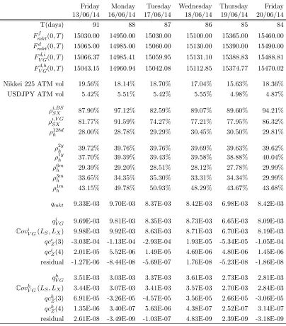
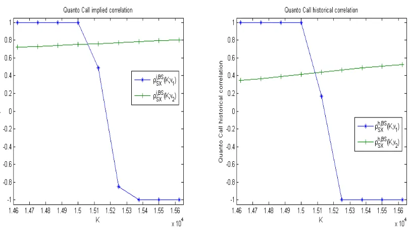
In this section, we aim at testing the consistency of the two calibration procedures introduced in Section 4.1 through the pricing of Quanto options on the Nikkei 225 index. Due to the fact that in our framework these products can be easily priced via analytical formulas (up to a Fourier inversion), these prices can be used to back out the relevant correlation. However, although market quotes for Quanto options are available from the CME platform, we do not have access to them and therefore we base our analysis on model prices obtained using the parameters recovered from both calibration procedures and reported in Table 2. Then, we can recover the value of the correlation coefficient such that the computed Quanto call option prices are matched by the ones obtained in the Black-Scholes model. To this purpose, though, we need first to carefully deal with the volatility smile/skew effect. Common market practice is, in fact, to use the at-the-money implied volatility for both the Nikkei 225 index, and the USDJPY FX spot rate, reported in Table 1. Pricing of multi-asset options, such as Quanto options, though requires consistency with the volatility smile of the corresponding assets (see also Shevchenko, 2006). This is evident when we use Equation (17) with Qadj = 1 in the Black-Scholes setting to recover the correlation coefficient value such that the Quanto call prices generated by the multivariate VG model are matched exactly. Results are presented in Figure 4, in which we show the implied correlation coefficient extracted from the Black-Scholes model under the assumption that the volatility of both the Nikkei 225 index and the USDJPY FX rate is set at the corresponding at-the-money value, and under the assumption that the volatility smile of the index is incorporated in the procedure. In details, in the left hand panel of Figure 4, we illustrate the case in which the input Quanto option prices are generated using the parameters from the QF-based calibration; we denote the resulting implied correlation coefficients as ρi,BS_SX (K;v1) if at-the-money volatilities are used, and

ρi,BS_SX (K;v2) if the whole volatility smile is incorporated instead. Similarly, in the right hand panel of Figure 4 we report the same quantities obtained from input prices generated by the parameters from the HC-based calibration; we denote these coefficients asρh,BS_SX (K;v1) andρh,BS_SX (K;v2). We note that when input prices are generated with the at-the-money volatilities, implied correlation values are close to their admissible bounds [−1,1] regardless of the calibration approach adopted; this in turn generates a pronounced mispricing of in-the-money and out-of-the-money options (results available upon request). If instead the volatility smile is used, the resulting implied correlation values show an increasing pattern from 70.91% to 79.54% in the case of input parameters obtained from the QF-based calibration, and 34.74% to 52.76% in the case of input parameters from the HC-based calibration.

Hence, from this simple experiment, we observe that once the volatility smile of the underlying asset is correctly taken into account, information extracted from historical prices generates inconsistent estimates of the correlation value; by using the parameters obtained from the HC-based calibration, in fact, we would expect to recover values of the correlation close to the historical estimate of 28% used in the calibration. This procedure instead generates a discrepancy in the correlation value ranging from 58% to 88%. The parameters obtained from the QF-based calibration, on the other hand, generate values of the correlation relatively close to the one originated by the Quanto futures quotes, as the (percentage) difference ranges from 3% to 13%.

4.3 Tail dependence and risk measures

the case in our particular example discussed in the previous sections. Hence, we use Equations (3) and (4), derived in Section 2 to compute the indices of upper and lower tail dependence between the log-returns of the Nikkei 225 index and the USDJPY FX rate using the calibrated multivariate VG model; corresponding analytical expressions are recovered following a similar argument as in Barndorff-Nielsen and Shiryaev (2010)2. We consider a 1 week horizon. We use the parameters obtained from both calibration procedures described in Section 4.1. Results are shown in Figure 5, from which we note that both calibrated VG models produce a non negligible tail dependence effect. Specifically, in light of the previous discussion, we observe that correlated downwards jumps are more likely according to the prevailing market expectations than what experienced in the past, as the index of lower tail dependence (in the right hand panel of Figure 5) is significantly higher when the parameters of the systematic risk process are recovered from Quanto futures. In other words, information from historical prices leads to underestimating the probability of a joint downward movement; this effect could have an impact on potential capital requirements linked to this measure of risk.

The two alternative correlation assumptions underpinning the calibration approaches discussed in this section also have an influence on univariate contracts. This is evident, for example, in the computation of the Value-at-Risk (VaR) of positions in non linear contracts, as vanilla call options, defined as the potential loss given a prespecified level of probability due to market movements. We illustrate the point by computing the 95% VaR for a short position in one call option on the Nikkei 225 index over both a 1 day and 10 days exposure periods (this example is inspired by Eberlein et al., 1998). Results are presented in Figure 6, which shows that the 95% VaR is higher under the QF-implied calibration procedure, due to the fact that the resulting distribution of the Nikkei 225 index has a relatively heavier right tail, implying relatively more likely upwards movements in the index. In other words, similarly to the case of joint downward risk, information extracted from historical prices could lead to underestimating the risk of losses for sell side market participants, again with cascading effects on potential capital requirements linked to these positions. Similar results can be obtained for alternative levels of confidence.

5

Conclusion

In this paper, we have developed a multivariate L´evy model for the joint dynamics of FX exchange rates and asset prices based on the factor representation of Ballotta and Bonfiglioli (2014). In this setting, we consider the pricing and calibration of Quanto contracts of vanilla nature which are traded over-the-counter in significant size, with the aim of extracting information about the dependence in place. In particular, as in our model Quanto call options can be related to European call options, fast and accurate pricing of these products is achieved via Fourier inversion techniques.

The numerical analysis presented in Section 4 for the CME USD-denominated Quanto futures on the Nikkei 225 index have shown the impact on prices of derivative contracts of different assumptions on the correlation coefficient linking the index to the USDJPY FX rate. In particular, we have shown that the correlation implied by Quanto futures and Quanto options can be quite different (always greater in this empirical example) from the historical correlation and DCC. This has a particular impact on the indices of upper and lower tail dependence and on the computation of risk measures related to portfolios containing these products: information based on historical correlation leads to underestimating both the probability of a joint downward movement in the relevant assets, and the VaR of short positions in the derivative contracts under consideration. Further, as in the proposed construction the quanto adjustment is affected by higher order cumulants of the pure jump part of the systematic risk factor, we are able to estimate the contribution of the skewness, the excess kurtosis

2

and the higher order terms. The empirical analysis reveals the predominant role of the skewness of the distribution of the common risk factor, covariance aside.

As the proposed model is based on L´evy processes, i.e. processes with independent and station-ary increments, stochastic volatility effects are ignored. For the case of the analysis considered in this paper, this is acceptable due to the very short maturities of the contracts involved. However, stochastic volatility effects can be added in our framework by using an analogous model based on multidimensional versions of time changed L´evy processes; in particular it would be interesting to allow dependence between the stochastic clock and the basis L´evy process: according to e.g. Carr and Wu (2004), this would model more adequately the observed features of stochastically varying return volatilities and correlation. Another aspect not considered in this paper is the simultaneous calibration of FX triangles. These topics are left however to future research.

Acknowledgments

The authors would like to thank H. Albrecher, A. Consiglio, E. Eberlein, G. Fusai, M. Grasselli, W. McGhee and U. Wystup for their constructive suggestions and comments; further thanks go to H. Vander Elst for his help with DCC. A previous version of this work has been circulated with the title ‘Pricing derivatives written on more than one underlying asset in a multivariate L´evy framework’. Results have been presented to the 8th World Congress of the Bachelier Finance Society, the Colloque ‘Journ´ees actuarielles de Strasbourg’, the 2nd European Actuarial Journal Conference, the 2015 Actuarial and Financial Mathematics Conference, the Conference in ‘Challenges in Derivatives Markets: Fixed income modelling, valuation adjustments, risk management, and regulation’, the Lorentz Center Workshop ‘Models and Numerics in Financial Mathematics’ and the 2015 AMASES Conference. We thank all participants for their useful feedback. This research was partly carried out while Griselda Deelstra and Gregory Rayee were visiting Cass Business School. Griselda Deelstra acknowledges support of the ARC grant IAPAS “Interaction between Analysis, Probability and Actuarial Sciences” 2012-2017. Gr´egory Ray´ee is supported by a Mandat de Charg´e de Recherche from the Fonds National de la Recherche Scientifique, Communaut´e fran¸caise de Belgique. Usual caveat applies.

References

Atanasov, V., Nitschka, T., 2015. Foreign currency returns and systematic risks. Journal of Financial and Quantitative Analysis 50, 231–250. http://dx.doi.org/10.1017/S002210901400043X.

Ballotta, L., Bonfiglioli, E., 2014. Multivariate asset models using L´evy processes and applications. The European Journal of Financehttp://dx.doi.org/10.1080/1351847X.2013.870917.

Ballotta, L., Fusai, G., 2015. Counterparty credit risk in a multivariate structural model with jumps. Finance, Revue de l’Association Fran¸caise de Finance 36.

Barndorff-Nielsen, O.E., Shiryaev, A., 2010. Change of time and change of measure. volume 13 of Advanced Series on Statistical Science and Applied Probability. World Scientific.

Basel, 2010. Basel III: A global regulatory framework for more resilient banks and banking systems. http: //www.bis.org/publ/bcbs189.pdf.

Branger, N., Muck, M., 2012. Keep on smiling? The pricing of Quanto options when all covariances are stochastic. Journal of Banking & Finance 36, 1577 – 1591. http://dx.doi.org/10.1016/j.jbankfin. 2012.01.004.

Carr, P., Wu, L., 2004. Time-changed L´evy processes and option pricing. Journal of Financial Economics 71, 113–141.

Carr, P., Wu, L., 2007. Stochastic skew in currency options. Journal of Financial Economics 86, 213–247.

Chicago Board Options Exchange, 2009. CBOE S&P Implied Correlation Index.http://www.cboe.com/micro/ impliedcorrelation/ImpliedCorrelationIndicator.pdf.

Co, R., Kerpel, J., Labuszewski, J.W., 2013. Nikkei 225 Spread Opportunities. Technical Report. CME Group.

Cont, R., Tankov, P., 2004. Financial modelling with Jump Processes. Chapman & Hall/CRC Press.

Da Fonseca, J., Grasselli, M., Tebaldi, C., 2007. Option pricing when correlations are stochastic: an analytical framework. Review of Derivative Research 10, 151–180.

De Col, A., Gnoatto, A., Grasselli, M., 2013. Smiles all around: FX joint calibration in a multi-Heston model. Journal of Banking & Finance 37, 3799 – 3818. http://dx.doi.org/10.1016/j.jbankfin.2013.05.031.

Eberlein, E., Frey, R., von Hammerstein, E.A., 2008. Advanced credit portfolio modeling and CDO pricing., in: J¨ager, W., Krebbs, H.J. (Eds.), Mathematics Key Technology for the Future. Springer, pp. 253–279.

Eberlein, E., Keller, U., Prause, K., 1998. New insights into smile, mispricing, and Value at Risk: The Hyperbolic model. The Journal of Business 71, 371–405.

Eberlein, E., Papapantoleon, A., Shiryaev, A.N., 2009. Esscher transform and the duality principle for multidi-mensional semimartingales. The Annals of Applied Probability 19, 1944–1971. 10.1214/09-AAP600.

Embrechts, P., McNeil, A., Straumann, D., 2002. Correlation and dependence in risk management: properties and pitfalls, in: Dempster, M. (Ed.), Risk management: Value at Risk and beyond. Cambridge University Press, pp. 176–223.

Engle, R., 2002. Dynamic conditional correlation: A simple class of multivariate generalized autoregressive conditional heteroskedasticity models. Journal of Business & Economic Statistics 20, 339–350.

Fang, F., Oosterlee, C., 2009. Pricing early-exercise and discrete barrier options by fourier-cosine series expan-sions. Numerische Mathematik 114, 27–62.

Geman, H., El Karoui, N., Rochet, J., 1995. Changes of num´eraire, changes of probability measure and option pricing. Journal of Applied Probability 32, 443–458.

Gerber, H.U., Shiu, E.S.W., 1994. Option pricing by Esscher transforms. Transactions of Society of Actuaries 46, 99–140.

Giese, A., 2012. Quanto adjustments in the presence of stochastic volatility. Risk 25, 67– 71.

Glasserman, P., 2003. Monte Carlo Methods in Financial Engineering. Springer-Verlag, New-York.

Hubalek, F., Sgarra, C., 2006. Esscher transforms and the minimal entropy martingale measure for exponential L´evy models. Quantitative Finance 6, 125–145. http://dx.doi.org/10.1080/14697680600573099.

Itkin, A., Lipton, A., 2015. Efficient solution of structural default models with correlated jumps and mutual obligations. International Journal of Computer Mathematics Forthcoming. http://dx.doi.org/10.1080/ 00207160.2015.1071360.

Lipton, A., Sepp, A., 2009. Credit value adjustment for credit default swaps via the structural default model. The Journal of Credit Risk 5, 127–150.

Lucic, V., 2012. Correlation skew via product copula, in: Financial Engineering Workshop, Cass Business School.

Madan, D.B., Carr, P., Chang, E., 1998. The Variance Gamma process and option pricing. European Finance Review 2, 79–105.

Madan, D.B., Milne, F., 1991. Option pricing with VG martingale components. Mathematical Finance 1, 39–45.

Madan, D.B., Seneta, E., 1990. The Variance Gamma (VG) model for share market returns. Journal of Business 63, 511–524.

Oh, D.H., Patton, A.J., 2012. Modelling dependence in high dimensions with factor copulas.

Sato, K., 1999. L´evy Processes and Infinitely Divisible Distributions. volume 68 of Cambridge Studies in Advanced Mathematics. Cambridge University Press.

Shevchenko, P.V., 2006. Implied correlation for pricing multi-FX options. Derivatives Week , 8–9, 10–11.

Tankov, P., 2004. L´evy process in finance: Inverse problems and dependence modelling. Ph.D. thesis. Ecole Polytechnique, Paris.

A

Proofs of results

A.1 Proof of Proposition 1

Leta= (a1,· · · , an)>, and assume thatΛ(t) has generating triplet (β,Γ, ν). It follows from Sato (1999, E12.10)

(see also Cont and Tankov, 2004, Proposition 5.3) thatβ = (β1, ..., βn, βZ)>, Γ is diagonal and ν is supported

by the union of the coordinate axes. Define an×(n+ 1) matrixM as

M =



   

1 0 ... 0 a1

0 1 ... 0 a2

..

. ... ... ... ... 0 0 ... 1 an



   

.

ThenL(t) =MΛ(t); it follows from Sato (1999, Proposition 11.10) (see also Cont and Tankov, 2004, Theorem 4.1) that L(t) is a L´evy process with drift and diffusion matrix as given. The characteristic function follows from the independence of the components of Λ(t). For the construction of the L´evy measure, we note that

{a∆Z(t)6= 0,a∆Z(t)∈B}if and only if{∆Z(t)6= 0,∆Z(t)∈A}. As the components ofΛ(t) are independent, Sato (1999, E12.10) implies that the support ofκis the union of the coordinate axes and the result follows. See Tankov (2004) as well.

A.2 Proof of Corollary 2

Results for γLj, c2j follow from Cont and Tankov (2004, Proposition 5.2); the L´evy measure follows from Cont

and Tankov (2004, Proposition 5.3) and Sato (1999, E12.10) by recognizing that Lj(t) = Yj(t) +ajZ(t) and

Yj(t) is independent ofZ(t).

A.3 Proof of Proposition 3

a) Applying the above, we obtain

P(Lj(t)< lj, Lk(t)< lk) = P(Yj(t) +ajZ(t)< lj, Yk(t) +akZ(t)< lk) ' _P(ajZ(t)< lj, akZ(t)< lk) lj, lk↓ −∞.

Hence, ifaj, ak >0

P(Lj(t)< lj, Lk(t)< lk)'P

Z(t)<min

lj

aj

, lk ak

lj, lk↓ −∞,

whilst, ifaj, ak<0

P(Lj(t)< lj, Lk(t)< lk)'P

Z(t)>max

lj aj , lk ak

lj, lk ↓ −∞.

On the other hand, ifρL

jk<0 for allt >0, we obtain

P(Lj(t)< lj, Lk(t)< lk)'P

Z(t)>

lj aj

, Z(t)< lk ak

lj, lk ↓ −∞

ifaj<0< ak, and

P(Lj(t)< lj, Lk(t)< lk)'P

Z(t)< lj aj

, Z(t)>

lk ak

lj, lk ↓ −∞

ifak<0< aj; therefore both probabilities are equal to zero.

b) The result follows by the same argument as above.

c) We note that ρL

jk <0 if and only if either aj <0 < ak orak <0< aj. Let us consider first the case in

whichaj<0< ak; then

P(Lj(t)< lj, Lk(t)> lk) ' P(−ajZ(t)>|lj|, akZ(t)> lk) |lj|, lk ↑ ∞. (A.1)

Asaj <0, then

P(Lj(t)< lj, Lk(t)> lk) ' P

Z(t)>max

lj aj

, lk ak

|lj|, lk ↑ ∞.

On the other hand, ifak<0< aj, by similar argument we obtain

P(Lj(t)< lj, Lk(t)> lk) ' P

Z(t)<min

_l j

aj

,− lk |ak|

.

If we have positive correlation, i.e. aj, ak >0, then Equation (A.1), would read as

P(−ajZ(t)>|lj|, akZ(t)> lk)'P

Z(t)<− lj aj

, Z(t)> lk ak

|lj|, lk ↑ ∞

which is zero, as the event is impossible. Similar argument applies whenaj, ak<0.

A.4 Proof of Proposition 4

The Girsanov theorem implies that the change of measure is in this case governed by the Esscher parameter

hj ∈R, which is constant by construction. Consequently the processesΛ(t) and L(t) remain L´evy processes

underPhj. Therefore, part (a) follows directly from the Girsanov theorem. Part (b) follows from Proposition 1

Nikkei 225 USDJPY

Spot S(0) 15097.84 JPY X(0) 102.03 JPY/USD

ATM implied volatility 19.56% 5.42%

Japan risk free rate of interest rf 0.10% US risk free rate of interest rd 0.25%

Nikkei 225 futures Ff(0, T) 15030 JPY Nikkei 225 Quanto futures Fd(0, T) 15065 USD

T 91 days

Historical correlation ρh_SX 28%

Table 1: Synopsis of market data. Source: Bloomberg, CME free web platform (see http://www.cmegroup.com/). Observation date: June 13, 2014. rf, rd: benchmark interest rates

of Japan and US, respectively. ρh

SX : historical correlation between log-returns estimated on a sample

QF-based calibration HC-based calibration

Idiosyncratic process Systematic process Idiosyncratic process Systematic process

Nikkei 225 USDJPY Nikkei 225 USDJPY

θYS -0.0177 θYX 0.1514 θZ -0.1830 θYS -0.3825 θYX -0.1362 θZ 0.5978 σYS 0.0150 σYX 0.0070 σZ 0.1095 σYS 0.1661 σYX 0.0294 σZ 0.0956 κYS 0.0084 κYX 0.0449 κZ 0.0522 κYS 0.0750 κYX 0.0456 κZ 0.0307

aS 1.8110 aX 0.4008 aS 0.6158 aX 0.2776

RMSRE 6.91E-03 RMSRE 6.33E-03

Margin process Systematic process Margin process Systematic process

Nikkei 225 USDJPY Nikkei 225 USDJPY

ELS(1) -0.3491 ELX(1) 0.0781 EZ(1) -0.1830 ELS(1) -0.0144 ELX(1) 0.0297 EZ(1) 0.5978 p

VarLS(1) 0.2129 p

VarLX(1) 0.0573 p

VarZ(1) 0.1172 pVarLS(1) 0.2149

p

VarLX(1) 0.0571 p

VarZ(1) 0.1418

s(L_S(1)) -0.2324 s(L_X(1)) -0.0495 s(Z(1)) -0.2341 s(L_S(1)) -0.2814 s(L_X(1)) -0.0393 s(Z(1)) 0.3173

κ(LS(1)) 0.1920 κ(LX(1)) 0.1165 κ(Z(1)) 0.1940 κ(LS(1)) 0.2379 κ(LX(1)) 0.1030 κ(Z(1)) 0.1649

ρi,V G_SX 81.77% ρh,V G_SX 28.00%

Table 2: Top panel - Calibrated parameters of the multivariate VG model. QF-based calibration: Z, aS, aX calibrated using Quanto

futures quotes. HC-based calibration: Z,aS,aXcalibrated using historical correlation (128 days). Bottom panel - Moments of the resulting

margin distribution. ρi,V G_SX : pairwise correlation coefficient computed using Equation (2) and the QF-based calibrated parameters. ρh,V G_SX : recovered pairwise historical correlation. sandκdenote the indices of skewness and excess kurtosis as in Cont and Tankov (2004). Data: see Table 1.

Friday Monday Tuesday Wednesday Thursday Friday 13/06/14 16/06/14 17/06/14 18/06/14 19/06/14 20/06/14

T(days) 91 88 87 86 85 84

F_mktf (0, T) 15030.00 14950.00 15030.00 15100.00 15365.00 15460.00

Fd

mkt(0, T) 15065.00 14985.00 15060.00 15130.00 15390.00 15490.00

F_{V G}d,i(0, T) 15066.37 14985.41 15059.95 15131.10 15388.83 15488.81

F_{V G}d,h(0, T) 15043.15 14960.94 15042.08 15112.85 15374.77 15470.02

Nikkei 225 ATM vol 19.56% 18.14% 18.70% 17.04% 15.63% 18.36%

USDJPY ATM vol 5.42% 5.51% 5.42% 5.55% 4.98% 4.87%

ρi,BS_SX 87.90% 97.12% 82.59% 89.07% 89.60% 94.21%

ρi,V G_SX 81.77% 91.59% 74.27% 77.21% 77.95% 86.32%

ρ128d

h 28.00% 28.78% 29.29% 30.45% 30.50% 29.81%

ρ2_hy 39.72% 39.76% 39.76% 39.69% 39.63% 39.62%

ρ1_hy 37.70% 39.39% 39.43% 39.58% 38.88% 40.04%

ρ6_hm 29.39% 29.20% 28.51% 28.12% 27.78% 29.99%

ρ3m

h 33.65% 34.35% 35.30% 33.31% 34.34% 29.99%

ρ1m

h 43.15% 49.78% 50.93% 48.29% 43.67% 43.68%

qmkt 9.33E-03 9.70E-03 8.37E-03 8.42E-03 6.98E-03 8.42E-03

qi

V G 9.69E-03 9.81E-03 8.35E-03 8.73E-03 6.65E-03 8.09E-03 CoviV G(LS, LX) 9.98E-03 9.92E-03 8.63E-03 8.71E-03 6.70E-03 8.19E-03

qci_Z(3) -3.03E-04 -1.13E-04 -2.93E-04 1.93E-05 -5.34E-05 -1.05E-04

qci_Z(4) 2.01E-05 5.52E-06 1.49E-05 4.69E-06 4.80E-06 1.45E-06 residual -1.27E-06 -8.44E-08 -5.69E-07 1.76E-08 -5.23E-08 -1.86E-08

qh

V G 3.51E-03 3.03E-03 3.37E-03 3.61E-03 2.73E-03 2.81E-03 CovhV G(LS, LX) 3.44E-03 3.07E-03 3.41E-03 3.57E-03 2.70E-03 2.84E-03

qch_Z(3) 6.91E-05 -3.26E-05 -4.57E-05 3.56E-05 2.66E-05 -3.06E-05

qch_Z(4) 1.35E-06 3.40E-07 5.63E-06 4.38E-07 2.52E-07 3.14E-07 residual 2.61E-08 -3.49E-09 -1.03E-07 4.83E-09 2.39E-09 -3.18E-09

Table 3: Time evolution analysis -Fd

mkt(0, T): USD-denominated CME Nikkei 225 futures quote

(sym-bol: NKD).F_mktf (0, T): JPY-denominated CME Nikkei 225 futures quote (symbol: NIY).F_{V G}d,i(0, T): USD-denominated Nikkei 225 futures quote computed with Equation(20)-(21)and QF-based calibration parameters. F_{V G}d,h(0, T): USD-denominated Nikkei 225 futures quote computed with Equation (20) -(21)and HC-based calibration parameters. qmkt: quanto adjustment implied by market data. qV Gi and

CovV Gi (LS, LX): quanto adjustment and covariance computed with QF-based calibration parameters.

qh

V G and CovhV G(LS, LX): quanto adjustment and covariance computed with HC-based calibration

Figure 1: USDJPY and Nikkei 225 implied volatility in function of strike K: market vs calibrated multivariate VG model. Options market data, June 13, 2014: Source: Bloomberg. USDJPY Options maturity: T = 1month. Nikkei 225 Options maturity: T = 28days (July 11, 2014). Market Data: Table 1. Multivariate VG model parameters: Table 2, QF-based calibration.

Figure 2: Evolution of the correlation spread in function of time t (in days). Starting date (t=0): June 13, 2014. MaturityT: September 12, 2014. Nikkei 225 indexS(t)market data, June 13, 2014 -September 12, 2014: Source: Bloomberg. Ff_{(t, T): futures prices computed by using Equation(10),}

rf = 0.10%. Fd(t, T)(ρiSX)andF

d_{(t, T)(ρ}h

SX): Quanto futures prices computed by using Equation

Figure 3: Dynamic Conditional Correlation between USDJPY and Nikkei 225 index log-returns (using daily data from January 2000-February 2015).

Figure 4: Left hand panel: QF-based calibration. Right hand panel: HC-based calibration. ρ·_SX,BS(K;v1): Quanto call implied correlation in function of strikeK, extracted in a BS setting where

the Nikkei 225 index and the USDJPY FX rate volatility are set at their at-the-money values (see Table 1). ρ·_SX,BS(K;v2): Quanto call implied correlation in function of strike K, extracted in a BS setting

Figure 5: Upper and Lower Tail dependence for given percentage variations of the log-returns (on a log-scale). QF Corr: QF-based calibration. h Corr: HC-based calibration. Parameters: Table 2.