City, University of London Institutional Repository
Citation
:
Radicchi, F. & Baronchelli, A. (2012). Evolution of optimal Lévy-flight strategies
in human mental searches. Physical Review E - Statistical, Nonlinear, and Soft Matter
Physics, 85(6), doi: 10.1103/PhysRevE.85.061121
This is the unspecified version of the paper.
This version of the publication may differ from the final published
version.
Permanent repository link:
http://openaccess.city.ac.uk/2655/
Link to published version
:
http://dx.doi.org/10.1103/PhysRevE.85.061121
Copyright and reuse:
City Research Online aims to make research
outputs of City, University of London available to a wider audience.
Copyright and Moral Rights remain with the author(s) and/or copyright
holders. URLs from City Research Online may be freely distributed and
linked to.
City Research Online:
http://openaccess.city.ac.uk/
[email protected]
arXiv:1204.2485v2 [physics.soc-ph] 20 Jun 2012
Evolution of optimal L´
evy-flight strategies in human mental searches
Filippo Radicchi1,∗ and Andrea Baronchelli2,†
1
Departament d’Enginyeria Quimica, Universitat Rovira i Virgili, Av. Paisos Catalans 26, 43007 Tarragona, Catalunya, Spain
2
Laboratory for the Modeling of Biological and Socio-technical Systems, Northeastern University, Boston MA 02115 USA
(Dated: June 21, 2012)
Recent analysis of empirical data [F. Radicchi, A. Baronchelli & L.A.N. Amaral. PloS ONE 7, e029910 (2012)] showed that humans adopt L´evy flight strategies when exploring the bid space in on-line auctions. A game theoretical model proved that the observed L´evy exponents are nearly optimal, being close to the exponent value that guarantees the maximal economical return to players. Here, we rationalize these findings by adopting an evolutionary perspective. We show that a simple evolutionary process is able to account for the empirical measurements with the only assumption that the reproductive fitness of the players is proportional to their search ability. Contrarily to previous modeling, our approach describes the emergence of the observed exponent without resorting to any strong assumptions on the initial searching strategies. Our results generalize earlier research, and open novel questions in cognitive, behavioral and evolutionary sciences.
PACS numbers: 05.40.Fb, 02.50.Le, 87.23.Ge
I. INTRODUCTION
L´evy flights are a special class of random walk whose step lengths follow a power-law tailed distribution [1]. They have been proved to be the most efficient type of space ex-ploration that can be adopted by a random searcher look-ing for scarce resources in an unknown environment [2]. Probably for this reason, there are plenty of empirical evidences that movement patterns are compatible with L´evy flights in many different contexts where efficiency matters [3–12]. In particular, L´evy flights appear recur-rently in the description of the motion of animals in real space (see [13] for a review). Animals explore the en-vironment mainly for searching food resources, and it is therefore plausible to ascribe the optimality of their search strategies to a selective evolutionary process.
Recently, Radicchi et al. have provided empirical ev-idence that also human players participating in on-line auctions explore the bid space performing L´evy flights [15]. The exploration of the bid space represents a search process, but purely mental because performed in an abstract space. Interestingly, players adopt nearly op-timal L´evy flight exponents, in the sense that the values of the exponent used in real auctions are close to the one that maximizes their economic return. In [15], the search process in the bid space is studied as a game theoretical model, where the optimal exponent value corresponds to a Nash equilibrium [16].
Here, we propose an evolutionary model in which the reproductive fitness of the individuals is proportional to
∗Electronic address: [email protected] †Electronic address: [email protected]
their ability to win the auctions, and we show that the values of the L´evy flight exponents to which the model converges are very close to those measured in real data. This approach relaxes some of the assumptions made in the traditional game theoretical analysis, and deepens the understanding of the results: The optimality of the strategies adopted by bidders in on-line auctions can be seen as the outcome of a (evolutionary) learning process.
The paper is organized as follows. In section II, we pro-vide a detailed description of the type of auctions studied and modeled in this paper. Section III is devoted to the description of the model and its analytical treatment. In particular, section IIIA describes the case in which all players can choose only a bid value, while, in section IIIB, we generalize the model to the case in which players can place an arbitrary number of bids. Section IIIC is dedi-cated to the evolutionary game theoretical implementa-tion of the model. Secimplementa-tions IV and V are respectively devoted to the description of the numerical simulations of the model and to the estimation of the computational complexity needed to simulate or solve the model. In sec-tion VI, we provide a detailed descripsec-tion of the results of the model. Finally, in section VII, we draw our final comments and considerations.
II. LOWEST UNIQUE BID AUCTIONS
2
duration isa priorifixed and generally two or three weeks long. A bid can be any amount (in cents) from one cent to a certain maximum valueM, generally lower than one hundred dollars. For placing a bid, a player has to pay a fee, whose entity ranges from one to ten dollars depend-ing on the game. Durdepend-ing the auction, players know only the status of their own bids meaning whether they are winning or not. None of the players knows where the others have placed their bids until the end of the game. Multiple bids on the same value from the same player are allowed, but do not influence the outcome of the auction since a bid is considered as unique when a unique player has bid that value even if more than once. When the time dedicated to the auction expires, the winner is the player who made the LUB and can finally purchase the good for the value of the winning bid. For example, if at the end of the auction bid valuei= 1 is occupied by two bids (n1= 2), while n2= 3, n3= 1,n4 = 2 andn5 = 1 are the number of bids placed on valuesi = 2, 3, 4 and 5, respectively, then the winner is the player who has bid on value i = 3 because this is the lowest bid among all unique bid values.
A similar mechanism is also used in Highest Unique Bid (HUB) auctions. In this type of the games, the rules are the same as those of LUB auctions, with the only differ-ence that the winning value is the unmatched bid closest to the maximal bid value admitted in the game (i.e.,M). LUB and HUB auctions represent competitive arenas where players perform searches for a single target whose position is determined by the bids of the whole popu-lation. It is important to stress that, during the game, players are not aware of the values on which the other players have placed their bids, and therefore the explo-ration of the bid space of each player can be considered independent. Also, since the cost of each bid is much larger than the natural unit of the game (one cent), the number of steps that can be performed by a single player is limited and allows only a partial exploration of the bid space. Players need therefore good strategies in order to maximize their winning chances and simultaneously maintain limited their investments.
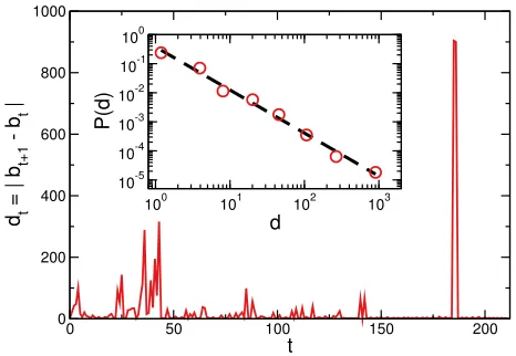
In our previous work [15], we have studied in detail the dynamical features of the bid space exploration per-formed by players in real LUB and HUB auctions. We have found that the exploration of the bid space is bursty: consecutive bid values are generally close to each other, but from time to time players perform longer jumps. In particular, the probability density function (pdf) P(d) of the bid change amount d (d is defined as the abso-lute value of the difference between two consecutive bid values) is consistent with a power-lawP(d)∼d−α (see Fig. 1). The exploration of the bid space is therefore consistent with a discrete version of a L´evy flight [14]. More importantly, we have found that the pdf g(α) of the L´evy flight exponents, adopted in real auctions, is peaked around the average value hαi ≃ 1.4 and with standard deviation equal toσ≃0.2.
0 50 100 150 200
t
0 200 400 600 800 1000
dt
=
|
bt+1
-bt
|
100 101 102 103
d
10-5 10-4 10-3 10-2 10-1 100
P(d)
Figure 1: (Color online) In the main panel, we plot dt the
absolute value of the difference between the two consecutive bid valesbt+1 and bt. t indicates the rank position of each bid in a ranking in which bids have been sorted accordingly to their time stamp. In the inset, we plot the pdfP(d) of the bid change amounts d (red circles). The pdf is fitted with a power-law function and the best estimate of the decay exponent is 1.5±0.1 (black dashed line). This figure refers to the exploration of the bid space performed by a single player in a single auction. A complete analysis of the movement patterns of hundreds of players was performed in our previous work [15].
The empirical observation of L´evy flights provided in [15] is by far the most significant evidence of this phenomenol-ogy in natural search processes. Differently from previ-ous studies regarding biological [2, 4–6, 10, 11] and mobil-ity [7, 8] systems where “two orders of magnitude of scal-ing can represent a luxury” [13] , the power-law decay can be clearly observed even over four orders of magnitude. The reason is that the space is not strictly physical and movements of tens of thousands cents can be performed at the same price of those one cent long: players explore the bid space in a effectivelysuper-diffusivefashion, and steps are made at a virtuallyinfinitevelocity.
III. MODELING BIDDING STRATEGIES
[image:3.595.323.556.50.211.2]Indepen-dently of the initial pdf, the pdf of the adopted expo-nents naturally evolves to a stable distribution centered around a value remarkably close to the one of the expo-nents measured in real auctions.
A. First bid
We consider a population ofN players whose strategies
αare randomly extracted from a pdfg(α). Without loss of generality, we assume that g(α) ≥0 if α∈ (α1, α2), and g(α) = 0 otherwise. During the game, each player can place bids only on integer values i ∈[1, M]. Since, at the beginning of the game, none of the players knows on which values the others will bid, it is natural to think that a generic player, with strategyα, sits at the leftmost site of the lattice. From this initial positions, the player places a bid on valueiwith probability
s(i, α) = i
−α
m(α) g(α) , (1)
where m(α) = PM
i=1 i−α is the proper normalization constant. The probability that a generic player bids on value i can be calculated by simply integrating Eq. (1) as
p(i) =
Z α2
α1
dα s(i, α) . (2)
After all players have bid, there will be nk bids on the
k-th bid value. The probability to observe a particular configuration {n} = (n1, n2, . . . , nk, . . . , nM) is simply given by the multinomial distribution
P({n}) =N!
M Y
k=1
[p(k)]nk
nk!
, (3)
whose weights given by Eq. (2) and obeying the con-straintN =PM
k=1 nk. In particular, the probability that only one bid has been made on value i (i.e., the bid on valueiis unique) is
u(i) = X
P
k6=ink=N−1
P({n}) =N p(i) [1−p(i)]N−1.
(4) The probability that the bid on value i is the unique and lowest bid can be exactly calculated by summing the probability of Eq. (3) over all configurations {n} which satisfy this constraint (i.e., ni = 1 and nj 6= 1 for all
j < i). Unfortunately, such enumeration cannot be easily
computed. A good approximation, valid for sufficiently low values ofp(i) andu(i), is to consider the uniqueness of thei-th bid value as independent of the uniqueness of the other bid values and write
l(i) =
u(i) , ifi= 1
u(i) Q
k<i [1−u(k)] , otherwise
, (5)
as the probability that the bid on valueiis the lowest bid among all the unique bids. The r.h.s. of Eq. (5) is the product of two terms: u(i) is the probability that only one bid has been made on bid valuei;Q
k<i [1−u(k)] is the probability that none of the bid values smaller than
i are occupied by a single bid (if i = 1 this probability is automatically equal to one sincei= 1 is the minimal bid amount allowed). Finally, the probabilityw(α) that the L´evy flight exponentαis the winning strategy in the game can be inferred with
w(α) =
M X
i=1
v(α|i) l(i) =
M X
i=1
s(i, α) l(i)
p(i) . (6)
v(α|i) = s(i, α)/p(i) is the conditional probability to observeαgiveni. This quantity is then convoluted over all bid valuesi, where the weight of each bid value is given by the probability thatiis the winning bid value, that is
l(i). Notice that Eqs. (4), (5) and (6) explicitly depend on the number of playersN and the upper bid valueM. We have suppressed both variables in the notation only for clarity and shortness.
B. Multiple bids
The same theoretical approach can be applied for the determination of the best strategy in a game where ev-ery player may perform multiple bids. We consider the simplest case in which each player bidsT times, but the theory may be simply extended also to the case in which the number of bids of each player is extracted from an arbitrary pdf.
In order to solve this game, we need to calculatesT(i) which stands for the probability that, inTbids, a generic player has placed a bid on value i. If αis the player’s strategy, the player will place the first bid on value i
with probability q1(i|α) = i−α/m(α). For the subse-quent bids, we need to define a transition matrix Qα. The generic element (Qα)jirepresents the probability to place a bid on valueiwhen the previous bid was placed on valuej. In our model, we have
(Qα)ji=|
i−j|−α
mj(α)
, (7)
for alli andj in the interval [1, M]. The normalization constantmj(α) =P
M
i=1|i−j|
−α
ensures the proper def-inition of the transition matrix. The matrixQαdescribes a random walker which follows uncorrelated L´evy flights with exponent α. At a generic step t, the probability that the player with strategyαsits on valueiis
qt(i|α) =
M X
j=1
4
The probability that this player placed a bid, inT bids, on valueiis then
sT(i|α) = 1− T Y
t=1
[ 1−qt(i|α) ] . (9)
The term 1−qt(i|α) counts the probability that the player has not placed a bid on value i at stage t. The probability that the player has not bid on valueiat any stage is therefore the product of this single step probabil-ities. Finally, the probability that the player has placed a bid on valueiat least once is calculated as the proba-bility to have bid on valueian arbitrary number of times minus the probability to have never bid on valuei. No-tice that the model assumes that players have no memory because they are allowed to bid on the same value more than once. This is, however, unlikely to happen in the L´evy and ballistic regimes (i.e., α <3). Also, as in the case of real auctions, if the same player bids more than once on the same value this fact does not invalidate the uniqueness of the bid which is still considered as unique unless another player places a bid on that value.
The probability that a generic player, performingT total bids, has placed a bid on valuei is then
pT(i) =
Z α2
α1
dα sT(i|α)g(α) (10)
and can be used in place of the one appearing in Eq.(2) in order to calculate the remaining quantitiesuT(i),lT(i) andwT(α) by using Eqs. (4), (5) and (6), respectively.
C. Evolutionary Model
In order to understand how an optimal strategy can be-come shared across individuals, it is natural to adopt an evolutionary framework [19]. In this respect, our model can be implemented in terms of competing individuals that are selected on the basis of their success in the searching process. In the spirit of the fundamental Moran process [20], at the end of each game, the winner of the auction generates an offspring to which transmits her/his search exponentα. The new individual enters the popu-lation endowed with an exponentα+ξ (withξ random mutation), while a randomly extracted individual is re-moved in order to maintain the population size constant. Basically, the pdf of the winning exponents of the for-mer generation corresponds to the fitness function of the evolutionary model.
1. Absence of mutations
Let us first consider the case in which losers copy the strategy of the winners without errors. Imagine to have
N players at each generation. They play the game by performing T bids each. Denote with e the number of
the generation. At the beginning, we sete= 1. Then we follow the scheme:
1. Players randomly pick strategies α from the pdf
g(e)(α);
2. They play the game. The result is the pdfw(Te)(α), which quantifies the probability thatαwas a win-ning strategy;
3. Setg(e+1)(α) =w(e)
T (α), incremente→e+ 1, and go back to point 1.
The former procedure describes the evolution of a population of players under repeated games. Setting
g(e+1)(α) =w(e)
T (α) ensures that the players of the new generation have the tendency to pick winning strategies instead of losing ones. This can be better understood by writing the master equation
g(e+1)(α)−g(e)(α) =
w(Te)(α)
1−g(e)(α)
−h1−wT(e)(α) i
g(e)(α) , (11)
from which one can easily obtain g(e+1)(α) = w(e) T (α). Eq. (11) tells us that the variation in the population of players with exponentαincreases as the probability that a player with strategyαwins [w(Te)(α)] times the proba-bility to have other players with strategies different from
α[1−g(e)(α)], and decreases as the probability that a player with strategy different fromαwins [1−w(Te)(α)] times the probability to find a player with strategy equal to α [g(e)(α)]. In other words, the probability of re-production of a player is proportional to the ability of player to win the game. The evolution rules resemble a Moran process where selection is made according to a fit-ness function here defined as the probability to win the game [20].
2. Random mutations
A more natural assumption is to formulate a model where, each time a losing player changes strategy, she/he copies the exponent of the winner plus some random vari-ation. Assume that the variationξis randomly extracted from a pdf y(ξ, α, ~µ), explicitly dependent on α and a set of parameters~µ. The master equation describing the evolution becomes
g(e+1)(α)−g(e)(α) =
+R
dβR
dξ δ(α−β+ξ) y(ξ, β, ~µ)×
wT(e)(β)
1−g(e)(β)
−h1−wT(e)(α)ig(e)(α)
,
0 1 2 3 4 5 α
0.0 0.2 0.4 0.6 0.8
w(
α
)
T = 10
T = 1
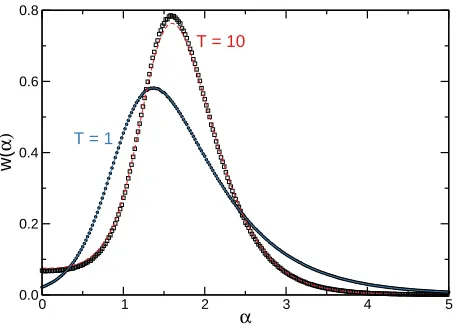
Figure 2: (Color online) Probability density function of the winning strategyw(α) in the case in which players’ strategies are randomly extracted from a uniform probability density functiong(α) defined over the interval (0,5). We setN= 100 andM = 1000 (parameter values similar to those observed in real auctions [15]), and consider for simplicity only the case of a single bidT = 1 and the case in which all players perform
T = 10 bids. We show in both cases the comparison between the results obtained with numerical simulations (T = 1 filled black circles,T= 10 empty black squares) and those obtained with the numerical integrations of the various equations [T = 1 full (lower) line, T = 10 dashed (upper) line]. Note that the optimal value ofαdepends onT and also the parameters valuesN and M. However, this is a weak dependence and the peak value of probability density function of the winning strategy is in the range 1.2 to 1.7 for a wide range of possible values ofN and M and a moderately broad range of values ofT.
the generic exponent β represents the winning strategy [w(Te)(β)] times the probability to have other players with exponent different fromβ[1−g(e)(β)]. This term is then convoluted with the noise over all possible values of β: this quantifies the probability that a random mutation changes the exponent from β to α [δ(α−β+ξ)]. The loss term is simply the probability thatαis not the win-ning strategy [1−w(Te)(α)] and therefore players with exponent α moves away from it at rate g(e)(α). The delta function imposes the condition α−β+ξ= 0 and the former equation reduces to
g(e+1)(α) =
+wT(e)(α)g(e)(α) +R
dβ y(β−α, β, ~µ) w(Te)(β)
1−g(e)(β)
. (12)
The pdf of the adopted strategies converges to stability whenever existse for which g(e+1)(α) = g(e)(α), which automatically implies thatw(Te+1)(α) =w(Te)(α).
IV. NUMERICAL SIMULATIONS
The former analytical formulation of the model does not allow to obtain explicit expressions regarding the distri-butions of the winning strategies. The various equations can, in fact, be only numerically integrated to provide a solution of the model. Moreover, some of the equations contain approximations, and it is therefore worth ask-ing whether the solutions obtained with the numerical integration of the equations are compatible with those obtained by directly simulating the model.
Simulating our model is straightforward. In each simu-lation, we use the following scheme:
1. Extract the exponent values of each of the N play-ers from the given pdfg(α);
2. Simulate the game: for each of the N players, ex-tractT integer bid values from the corresponding power-law distribution, and determine the winner of the auction (the player who made the LUB) on the basis of these extractions.
In the case of the evolutionary game model, at the end of the game we need to change the exponent value of one of the losing players, by copying (with or without random mutations) the strategy of the winner. We then repeat the game. A generation corresponds toN expo-nent changes. The pdf of the winning strategies of each generation is computed by repeating the entire procedure many times.
V. COMPUTATIONAL COMPLEXITY
One could argue why use a complicated and approxi-mated set of equations instead of simple and straightfor-ward numerical simulations. The reason is that the com-putational time required for the numerical integration of the model’s equations is much much lower than the one needed for obtaining good estimates with numerical sim-ulations. For clarity, we provide here an estimation of the computational complexity required in both approaches to the solution of the model.
[image:6.595.64.292.50.212.2]6
0 1 2 3 4 5
α
0.0 1.0 2.0 3.0 4.0
w
(e)
(
α
)
e = 5
e = 10
e = 20
e = 1
A
0 1 2 3 4 5
α
0.0 0.2 0.4 0.6 0.8 1.0 1.2
w
(e)
(
α
)
e = 2
e = 3
e = 1
C
e = 20
100 101 102 103
e
10-3
10-2
10-1
100
σ
λ= 0.0
λ= 2.0
λ= 5.0
0.0 0.5 1.0 1.5 2.0
<
α
>
B
100 101 102
e 0.0
0.2 0.4 0.6 0.8 1.0
σ
λ= 0.0
λ= 2.0
λ= 5.0
0.0 0.5 1.0 1.5 2.0
<
α
>
D
µ= 0.0
µ= 0.0
µ= 0.5
µ= 0.5
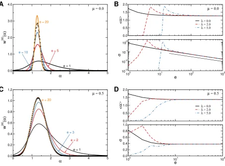
Figure 3: (Color online) Probability distribution function w(e)
(α) of the winning strategies at generation e. Here we set
M = 1000,N = 100 andT = 1. The mutationξis randomly extracted from a uniform distribution centered in zero and width 2µ: we consider the casesµ= 0.0 (panels A and B, absence of mutation) andµ= 0.5 (panels C and D). In A and C, the starting distribution for the exponents isg(1)(α) = 1/5 ifα∈ (0,5) and zero otherwise. Already after one generation (e= 1, lower black line), the peak of the distribution is aroundα≃1.5. As the number of generations increases, the distribution becomes more and even more peaked around a specific value of α, and reaches a stationary distribution. The asymptotic distribution has finite width forµ > 0, while is a delta function forµ = 0. As a term of comparison, we show also the results obtained with numerical aftere= 20 generations (black circles). In B and D, we consider initial distributions for the exponents of the typeg(1)(α)∼α−λ
if α∈(0,5) andg(1)(α) = 0 otherwise. We show the results for the three cases: λ= 0 (uniform, black full line),λ= 2 (power-law, red dashed line) andλ= 5 (exponential, blue dot-dashed line). The asymptotic distribution does not depend on the initial distribution and the peak value of the asymptotic probability density function does not depend on
µ. Independently of the value ofλ, as the number of generationseincreases, the average valuehαiand the standard deviation
σapproach the same stationary values: hαi ≃1.3 for anyµ, whileσ= 0 (as 1/√e, thin black line in panel B) forµ= 0.0 and
σ≃0.4 forµ= 0.5.
computational time that grows asM.
For general values ofT, the computational complexity of numerical simulations is simply incremented by a factor
Tand grows therefore asT M+T N log (M)G. The time required for the numerical integration of the equation dif-ferently grows as T M2. The most computationally ex-pensive calculation is the one of Eq. (8) that requires a time growing asM2, and this computation has to be repeatedT times.
VI. RESULTS
In all results, we consider the values N = 100 and
M = 1000. The choice of these parameter values is jus-tified because they are of the same order of magnitude as those measured in real auctions [15]. In Fig. 2, we plot the pdfw(α) forT = 1 andT = 10. In both cases,
[image:7.595.82.536.50.384.2]100 101 102 e
10-3
10-2
10-1
100
σ
λ= 0.0
λ= 2.0
λ= 5.0
0.0 0.5 1.0 1.5 2.0
<
α
>
B
100 101 102
e 0.0
0.2 0.4 0.6 0.8 1.0 1.2
σ
λ= 0.0
λ= 2.0
λ= 5.0
0.0 0.5 1.0 1.5 2.0
<
α
>
D
0 1 2 3 4 5
α
0.0 1.0 2.0 3.0 4.0 5.0
w
(e)
(
α
)
e = 5
e = 10
e = 20
e = 1
A
0 1 2 3 4 5
α
0.0 0.2 0.4 0.6 0.8 1.0 1.2 1.4
w
(e)
(
α
)
e = 2
e = 3
e = 1
C
e = 20
µ= 0.0 µ= 0.0
µ= 0.5
µ= 0.5
Figure 4: (Color online) Same as figure 3, but with different parameter values. Here we set M= 1000, N = 100 andT = 10, and considerµ= 0.0 in panels A and B, whileµ= 0.5 in panels C and D. The asymptotic pdf of the winning strategies have average valueshαi ≃1.5 for any value ofµ. The standard deviation isσ= 0 (as 1/√e) forµ= 0.0, andσ= 0.3 for µ= 0.5. For any value ofµ, the best strategy (i.e., the peak of the pdf) is placed atα∗
≃1.5.
that players don’t know which strategy is better for win-ning the game and all strategies are therefore a priori
equivalent. It is interesting to see that already in this situation there is a clear advantage for players that per-form L´evy flights and whose exponents are in the range 1.2−1.5. It is also worth noting that the solutions ob-tained with the numerical integration of the equations are perfectly consistent with the results obtained with numerical simulations.
More interesting is the case of evolutionary games. For simplicity, here we consider the case in which the distri-bution of the random mutations is a rectangular window of width 2µ: ifαis the winning strategy, the new expo-nent is equal to a random number taken from the uniform distribution into the interval (α−µ, α+µ). In the case in which the possible values of the exponents are bounded in the interval (α1, α2), we have to include the effect of the boundaries and write
y(ξ, α, α1, α2, µ) =
[ℓ1+ℓ2]−1 , if ξ∈(−ℓ1, ℓ2)
0 , otherwise ,
(13) where ℓ1 = min (α−α1, µ) and ℓ2 = min (α2−α, µ).
We show in Fig. 3 the results valid for T = 1 and in Fig. 4 those obtained for T = 10. These figures show results that are slightly different, but qualitatively iden-tical. The asymptotic pdfw(∞)(α) of the winning strate-gies does not depend on the initial distributiong(1)(α). In absence of mutation, the limiting pdf is a delta func-tion centered around an optimal strategy α∗. The con-vergence to such pdf is only asymptotic, since the width of the distribution goes to zero as 1/√eand is therefore finite at any finite generatione. If mutations are allowed (i.e., µ > 0), w(∞)(α) is reached after a finite number of iterations. The asymptotic distribution has a finite width. The number of iterations required to reach sta-bility depend on the initial pdf and the mutation rateµ, while its shape only onµ. In particular, the peak of the pdf is still atα∗, the same value as the one measured in absence of mutations. The value of α∗ depends on the parameters of the modelN,M andT but, for values con-sistent with those of real auctions (N = 50 toN = 200,
[image:8.595.82.536.52.383.2]8
VII. CONCLUSIONS
A large wealth of empirical evidences suggest that ani-mals have a specific, and apparently innate, strategy to search an unknown physical environment [13]. The dis-tances between two consecutive positions in the space are distributed according to a power-law probability density function. More interestingly, the exponent of the power-law distribution is close to the one that guarantees the most efficient search in an environment with scarce re-sources. Evolutionary considerations account for the high efficiency of the searching strategies of animals, since in a competitive environment only the fittest are able to survive and reproduce.
A similar behavior has been observed also in how human players explore the bid space in on-line auctions [15]. In this case, the environment is not physical but abstract. Nevertheless players adopt searching strategies for the winning bid value that are close to optimality: bid change amounts are power-law distributed, and the exponents of the power-laws are close to the value that can guarantee the highest winning chances.
In this paper, we have provided a novel interpretation of this empirical evidence and used evolutionary considera-tions to explain the optimality of the observed exponents. We have introduced a Moran-like model in which the re-productive fitness of the players is proportional to their success in searches [20]. The player winning the auction reproduces, in the sense that the strategy of the winner is transmitted to another randomly extracted individual. We have considered both the cases of error-free repro-duction and of transmission with mutation. We have
de-scribed the model analytically through a set of equations whose numerical solution is in excellent agreement with direct agent-based simulations. We have shown that the model is extremely robust with respect to the choice of the different parameters, producing results in good agree-ment with the ones observed in the empirical data.
In summary, looking at activity patterns in the web [21], our previous work [15] suggested that humans and other animals share the same, apparently innate, strategy to search in an unknown, physical or mental, environment. Here we have shown that an evolutionary approach allows to account for the optimality of the observed exponents, in agreement with the view according to which the abil-ity to understand and be effective in the natural world is likely to be innate [22]. This is the case for example of locomotion and perceptual-motor control [23], hunting and foraging [24] or nest building [25]. We have provided a new example with the remarkable novelty that it con-cerns a mental search process. While it is well known that humans share the intuition that numbers map into space [26], our work indicates that they might have de-veloped an innate knowledge about the best way to move in it.
Acknowledgments
The authors are indebted to Lu´ıs A. N. Amaral for help-ful discussions on the subject of this article. F. Radic-chi acknowledges support from the Spanish Ministerio de Ciencia e Innovaci´on through the Ram´on y Cajal pro-gram.
[1] M.F. Shlesinger, G.M. Zaslavsky & J. Klafter. Nature
363, 31–37 (1993).
[2] G.M. Viswanathanet al.Nature401, 911–914 (1999). [3] R. Mantegna & H.E. Stanley.Nature376, 46–49 (1995). [4] G.M. Viswanathanet al.Nature381, 413–415 (1996). [5] F. Bartumeus et al. Proc. Natl. Acad. Sci. USA 100,
12771–12775 (2003).
[6] G. Ramos-Fern´andez et al. Beahv. Ecol. Sociobiol. 55, 223–230 (2004).
[7] S. Bertrand, J.M. Burgos, F. Gerlotto, J. & Atiquipa. J. Mar. Sci.62, 477–482 (2005).
[8] D. Brockmann, L. Hufnagel & T. Geisel. Nature 439, 462–465 (2006).
[9] T. Rhodes & M.T Turvey. Physica A 385, 255–260 (2005).
[10] D.W. Simset al.Nature451, 1098–1102 (2008). [11] N.E. Humphrieset al.Nature465, 1066–1069 (2010). [12] G.M. Viswanathan.Nature465, 1018–1019 (2010). [13] G.M. Viswanathan, E.P. Raposo & M.G.E. da Luz. Phys.
Life Rev.5, 133–150 (2008).
[14] D.H. Hughes DH, M.F. Shlesinger & E.W. Montroll. Proc. Natl. Acad. Sci. USA78, 3287–3291 (1981). [15] F. Radicchi, A. Baronchelli & L.A.N. Amaral. PloS ONE
7, e029910 (2012).
[16] J. Nash, Proc. Natl. Acad. Sci. USA36, 48 (1950). [17] D.J.C. MacKay. Information Theory, Inference, and
Learning. (Cambridge University Press, Cambridge, 2003).
[18] G. Berkolaiko & S. Havlin. Phys. Rev. E55, 1395–1400 (1997).
[19] M.A. Nowak. Evolutionary Dynamics: exploring the equations of life. (Belknap Press of Harvard University Press, Cambridge MA, 2006).
[20] P.A.P. Moran. Math. Proc. Cambridge54, 60–71 (1958). [21] D. Lazer,et al.Science323, 721–723 (2009).
[22] N. Chater, N. & M.-H.Christiansen.Cognitive Sci.1–27 (2009).
[23] R.M. Alexander. Principles of animal locomotion. (Princeton University Press, Princeton, 2003).
[24] D.W. Stephens, J.S. Brown, & R.C. Ydenberg. Forag-ing: Behavior and ecology. (University of Chicago Press, Chicago, 2007).
[25] S.D. Healy, P Walsh. & M. Hansell.Curr. Biol.18, R271– R273 (2008).